THREE ESSAYS ON HOUSING MARKETS
A Dissertation
Presented to the Faculty of the Graduate School of Cornell University
In Partial Fulfillment of the Requirements for the Degree of Doctor of Philosophy
by Ziye Zhang August 2018
THREE ESSAYS ON HOUSING MARKETS Ziye Zhang, Ph. D.
Cornell University 2018
This dissertation contains three chapters related to housing markets. First two chapters study the vertical variation in housing prices, and the third chapter models buy-sellers. The first focus is the vertical dimension of housing markets. Location is the most important factor in determining housing prices. However, in multi-unit residential markets, two housing units in one building share the same location but may still have different transaction prices. The first chapter is to explore why. To identify the explanatory factors, the author collects over 200,000 transaction records from 2012-2016 in Beijing and provides rich and valid empirical evidence. Also, this chapter proposes a least nugget effects estimator (LNE) as an alternative to the conventional fixed effects estimator (FE). LNE is essentially a pairwise differences estimator (PD) whose comparison with FE in linear fixed effects models is studied in the second chapter.
The second focus of this dissertation is a type of households who are both home buyer and home seller at the same time (called “buy-sellers”). The traditional framework would model such households as two independent identities. However, this dichotomic tradition ignores the essential feature of the buy-sellers, that is, the interdependence between buying and selling decisions. As a buyer, a new purchase depends on a successful sale due to budget and policy restrictions; as a seller, a sale may rely on the success in bidding to avoid renting for a living. This interdependence results in a
connected bidding network. One’s success or failure in bidding or selling will influence others’. Chapter three, for the first time, studies this type of households and proposes an agent-based model (ABM) with buy-sellers. Then, the author uses this ABM to analyze the effects of housing purchase restrictions and home brokerage on market outcomes.
v
BIOGRAPHICAL SKETCH
The author was born in Beijing, China. He received his bachelor's degree in Public Policy and master's degree in Regional Economics from Peking University in 2011 and 2014. Later, he spent four years in Cornell University where he completed his Ph.D. in Regional Science. His research interests are urban housing markets, applied econometrics, and micro-simulation.
vi
vii
ACKNOWLEDGMENTS
I would like to express my deepest gratitude to my advisor, Dr. Kieran Donaghy, for his guidance, instruction, patience, and support. I would also like to thank my other committee members, Dr. Ricardo Daziano and Dr. Nancy Brooks, who constantly provide insightful feedback and suggestions on my research.
I would like to thank my wife, Yi Li. She is the best friend in my life and always being there supporting me, listening to my endless "housing stories", and cheering me up through tough times. I would never have been able to finish my dissertation without her standing by my side.
I would also like to thank my parents and my parents-in-law. They encourage me to pursue my interest in research and support me in the daily life.
Finally, I would like to thank my friends, Yuanshuo, Karina, Abhi, and Fikiri for their valuable suggestions and feedbacks for my research.
viii
TABLE OF CONTENTS
BIOGRAPHICAL SKETCH ··· v
TABLE OF CONTENTS ··· viii
LIST OF TABLES ··· x
LIST OF FIGURES ··· xi
CHAPTER 1 ··· 12
1.1 INTRODUCTION ··· 12
1.2 LITERATURE REVIEW ··· 15
1.2.1 Estimation of Structural Effects in MRMs ··· 15
1.2.2 Temporal Factors in MRMs ··· 17
1.2.3 Study and Practice in Beijing ··· 18
1.2.4 Fixed Effects Models in MRMs Studies ··· 19
1.3 METHODOLOGY ··· 20
1.3.1 Least Nugget Effect Estimator (LNE) ··· 20
1.3.2 Equivalency between LNE and Pairwise Differences Estimators (PD) ··· 21
1.3.3 PD Generalizes Fixed Effects Estimator (FE) ··· 22
1.3.4 Application in This Paper ··· 23
1.4 EMPIRICAL APPLICATION ··· 24 1.4.1 Study Area ··· 24 1.4.2 Data Source ··· 26 1.4.3 Variable ··· 28 1.4.4 Model Specification ··· 33 1.4.5 Result ··· 34
1.5 CONCLUSION AND DISCUSSION ··· 47
CHAPTER 2 ··· 49
2.1 INTRODUCTION ··· 49
2.2 PAIRWISE DIFFERENCES ESTIMATOR ··· 53
2.2.1 Model and Estimator ··· 53
2.2.2 PD Generalizes FE ··· 55
ix
2.3 COMPARISON BETWEEN FE AND PD ESTIMATOR ··· 57
2.3.1 Mediant and Weighted Mediant ··· 57
2.3.2 Relevant Theories from Mediant Theory ··· 58
2.3.3 Extension to Vector and Matrix ··· 58
2.4 A MONTE CARLO APPROACH ··· 60
2.4.1 Performance Tests Used in this Paper ··· 60
2.4.2 Monte Carlo Design ··· 61
2.4.3 Simulation Results ··· 67
2.4.4 Result Summary ··· 70
2.5 DISCUSSION AND CONCLUSION ··· 71
CHAPTER 3 ··· 87
3.1 INTRODUCTION ··· 87
3.1.1 Define Buy-sellers ··· 87
3.1.2 Resale Behavior and Dichotomic Tradition ··· 88
3.1.3 Bidding Network Insights ··· 88
3.1.4 Existence of Buy-sellers ··· 89
3.1.5 Agent-based Models ··· 90
3.2 A SIMPLE FRAMEWORK ··· 91
3.3 AGENT-BASED MODEL DESIGN ··· 92
3.4 HOUSING PURCHASE RESTRICTION AND HOME BROKERAGE ··· 105
3.4.1 Simulation Scenarios ··· 106
3.4.2 Outcome Measure··· 107
3.4.3 Model Setting ··· 107
3.4.4 Result ··· 107
3.4.5 A Dynamic View ··· 108
3.5 DISCUSSION AND CONCLUSION ··· 111
APPENDIX A DATA CLEANING AND OUTLIER DETECTION ··· 112
APPENDIX B RELATIONSHIP BETWEEN SUM SQUARED DIFFERENCES AND SUM SQUARED DEVIATIONS FROM THE MEAN ··· 117
APPENDIX C EQUIVALENCE AND DEVIATION CONDITIONS ··· 120
x
LIST OF TABLES
Table 1.1 Descriptive Statistics ... 32
Table 1.2 FE and LNE with Different Time Variables ... 35
Table 1.3 Estimates of Year Dummies ... 37
Table 1.4 FE Models with Interaction Terms ... 41
Table 1.5 Interaction among Floor Level, Elevator, and Total Floor ... 42
Table 2.1 Summary of Monte Carlo Simulation Designs* ... 62
Table 2.2 Monte Carlo Simulation Design ... 64
Table 2.3 Sample and Unbalancedness Design ... 66
Table 2.4 Mean Absolute Errors (Panel Setting) ... 73
Table 2.5 Mean Absolute Errors (Clustered Setting) ... 74
Table 2.6 Relative Mean Absolute Errors (PD/ FE) ... 75
Table 2.7 Mean Absolute Errors (Heteroscedasticity) ... 76
Table 2.8 Relative Mean Absolute Errors (Heteroscedasticity; PD/ FE) ... 76
Table 2.9 Change Rate % in Standard Error (Panel Setting) ... 77
Table 2.10 Change Rate % in Standard Error (Clustered Setting) ... 78
Table 2.11 Change Rate % in Standard Error (Heteroscedasticity) ... 81
Table 2.12 Rejection Rate (Default I.I.D., Nominal Size 0.05, Panel Setting) ... 82
Table 2.13 Rejection Rate (Default I.I.D., Nominal Size 0.05, Clustered Setting) ... 83
Table 2.14 Rejection Rate of CRVE (Nominal Size 0.05, Panel Setting) ... 84
Table 2.15 Rejection Rate of CRVE (Nominal Size 0.05, Clustered Setting) ... 85
Table 2.16 Rejection Rate when Heteroscedasticity ... 86
Table 3.1 Buy-seller Status ... 95
Table 3.2 Five Basic Types of Patterns ... 98
Table 3.3 Basic Combination of Two Pending Patterns ... 100
Table 3.4 Simulation Scenarios ... 107
Table 3.5 Total Number of Trades ... 108
Table 3.6 Average Time-on-market ... 108
xi
LIST OF FIGURES
Figure 1.1 Resale Housing Price and Population Indices (Year 2007 = 100) ... 26
Figure 1.2 Resale Transaction Volume (Units) and Market Share (%) of Lianjia ... 27
Figure 1.3 Population and Sample Sizes ... 28
Figure 1.4 Beijing Resale Housing Price (2012 Sample) ... 29
Figure 1.5 Beijing Resale Housing Price (2013 Sample) ... 29
Figure 1.6 Beijing Resale Housing Price (2014 Sample) ... 30
Figure 1.7 Beijing Resale Housing Price (2015 Sample) ... 30
Figure 1.8 Beijing Resale Housing Price (2016 Sample) ... 31
Figure 1.9 Estimates of Year Dummies ... 38
Figure 1.10 Vertical Gradient (with and without Elevator) ... 42
Figure 1.11 Vertical Gradient (with Elevator and Total Floors from 5 to 15) ... 43
Figure 2.1 Change Rate in Mean Standard Error (Panel Setting, 𝜌𝑥 = 0.5) ... 79
Figure 2.2 Change Rate in Mean Standard Error (Clustered Setting, 𝜌𝑥 = 0.5) ... 80
Figure 2.3 Change Rate in Mean Standard Error (Heteroscedasticity, 𝜌𝑥 = 0.5) ... 81
Figure 3.1 A Bidding Network Example ... 91
Figure 3.2 Successful Patterns with Buy-sellers ... 92
Figure 3.3 ABM ID Allocation ... 93
Figure 3.4 Flow Chart of Agents ... 96
Figure 3.5 Flow Chart of Bids ... 97
CHAPTER 1
VERTICAL VARIATION IN HOUSING PRICES—A LEAST NUGGET EFFECT APPROACH
1.1 INTRODUCTION
Multi-unit residential markets (MRMs) have been developed around the world1 and studied in many empirical hedonic analyses. One feature of these markets is the vertical variation in housing prices—that is, housing units in one building are transacted at different prices. Units in one building share the same location and neighborhood but may still differ in structural characteristics and transaction times. They could be on different floors, have different numbers of rooms, or face different directions. They could be transacted under different market conditions—prices may rapidly change in a housing boom or bust. Hence, the vertical variation in housing prices reflects people’s preference for the structural attributes and temporal fluctuation of housing prices.
Most hedonic analyses of MRMs identified the structural and temporal effects using overall price variations on both vertical and horizontal dimensions (e.g., Gao & Asami, 2011; Jim & Chen, 2009; Jim & Chen, 2010; Wong, So, & Hung, 2002; Wong, Chau, Yau, & Cheung, 2011), largely because in this way they could estimate the effects of location factors (e.g., accessibility and neighborhood quality)—which are always of the most interest. However, location factors are inherently complex and subject to misspecification in variables (Can, 1992; Dubin, 1992). They may induce measurement errors and omitted
1Evidence can be found in studies worldwide, such as Singapore (Sing, 2001; Sun, Tu, & Yu, 2005), Hong
Kong (Jim & Chen, 2009; Bao & Wan, 2004), Beijing (Ekblad & Werne, 1990), Tokyo (Kanemoto & Nakamura, 1986), Israel (Mitrany, 2005; Frenkel, 2007), US (Rosen & Walks, 2013), and large cities in Europe (Turkington, Van Kempen, & Wassenberg, 2004).
13
variable biases in parameter estimates (Kuminoff, Parmeter, & Pope, 2010). For some practices with primary interest in the structural and temporal factors—for example, designing floor plans of affordable housing projects or constructing housing price indices, the vertical dimension alone would provide better estimates than using overall variations because comparing housing units in one building naturally avoids the locational endogeneity issues. This paper uses the vertical information of the Beijing resale housing market from 2012 to 2016 to identify the explanatory variables for the vertical dimension.
Methodologically, to investigate housing price variation within one building, a conventional choice is to use the within model (fixed effects model) together with the fixed effects estimator (FE) 2, viewing the vertical variation as a particular type of within-group variation. In addition to applying FE, this paper explores another method using semivariograms. In spatial statistics, a semivariogram measures the variance of value differences between all pairs of observations with a certain distance apart (Cressie, 1993), which has been used in housing studies to model the spatial autocorrelation structure in error terms (Dubin, 1992; Basu & Thibodeau, 1998). When the distance between two observations in each pair tends to zero, the semivariogram is called the “nugget effect.” This paper uses this term and denotes the vertical variation in housing prices as the “nugget effect of housing prices”, because the vertical variation can be regarded as the variance of price differences between all pairs of housing transactions at the same location (i.e., with the certain distance apart tends to zero). To identify the explanatory variables for this
2It is also called within estimator or covariance estimator. In the context of clustered data, it is referred as
cluster-specific fixed effects estimator (Cameron & Miller, 2015). It is known that FE and the least squared dummy variable estimator (LSDV) estimator are computationally equivalent (Wooldridge, 2010), thus this paper will not discuss LSDV separately.
14
nugget effect, this paper estimates a linear hedonic price model by minimizing the nugget effect of residuals, instead of minimizing the overall sum of squared residuals as in OLS. The estimator is called a least nugget effect estimator (LNE) and is designed to explain most of the vertical variation of housing prices—rather than the overall variation.
Comparing FE and LNE, the essential difference is that FE measures the variation using the deviation from the mean in each group; while LNE uses the pairwise differences. This paper shows that the LNE is essentially a pairwise differences estimator (PD), whose comparison with FE in linear fixed effects models is studied in Chapter 2 of this dissertation. Chapter 2 shows that PD (and hence LNE) is a generalized version of FE by weighting each observation by its group size. When the data is balanced, i.e., each group has the same number of observations, or, when the local estimate of each group is the same, FE and PD are equivalent. For MRM housing data, the observed housing transactions are grouped by buildings, and this group structure is always unbalanced—buildings have different numbers of observations due to their differences in height, transaction frequency, and sample size. As a result, applying FE and PD would generate different results. Chapter 2 also shows that both FE and PD are unbiased and consistent. However, using cluster-robust standard errors, FE is more efficient than PD when the number of groups is large. This condition would be satisfied in MRMs when the number of buildings is massive. The empirical results of this paper provide evidence to the theoretical discussions.
In what follows, Section 1.2 reviews related literature, Section 1.3 introduces the estimation approaches; Section 1.4 applies the model to housing data in Beijing, and Section 1.5 concludes with key results.
15
1.2 LITERATURE REVIEW
Hedonic price models regress housing transaction prices3 on structural and spatial characteristics and on time variables (Butler, 1982; Freeman, 1981; Quigley, 1995; Tu, 1997). The regression coefficient of a variable is, ceteris paribus, the marginal change in the valuation of the housing unit (Rosen, 1974).
1.2.1 Estimation of Structural Effects in MRMs
For the structural charaterisitcs, literature on MRMs provides abundant empirical evidence on their estimates. Although the choice may differ by markets and regions, most studies involve several common structural variables, for example, floor areas, stories (floor level), number of rooms, views, orientations, and building age.
The floor area is the most common structural characteristic in hedonic housing studies (Sirmans, Macpherson, & Zietz, 2005). In the analyses of MRMs, the sign of the floor area depends on the choice of the price variable. Many studies use total selling prices and suggest a positive effect of the floor area (e.g., Chen, Clapp, & Tirtiroglu, 2011; Mason & Quigley, 1996; Xu, 2008; Yu, Han, & Chai, 2007); while some scholars find evidence of negative effects (Mok, Chan, & Cho, 1995) when using unit prices—the price per square foot (or meter), a common measure of the housing price in regions like Hong Kong and other cities in China.
The number of rooms is expected to correlate with the floor area. However, their effects on housing prices could be distinct. People may prefer housing units of a given floor area to be divided into more rooms (Borukhov, Ginsberg, & Werczberger, 1978). Positive
16
effect of the number of rooms is found in Tokyo (Shimizu, Takatsuji, Ono, & Nishimura, 2010) and Israel (Borukhov et al., 1978). Specifically, more bedrooms are associated with higher housing prices in Shenzhen, China (Xu, 2008) but with lower prices in Hong Kong (Jim & Chen, 2010). Some scholars include bedrooms as dummy variables to identify the most preferred number of bedrooms (e.g., Chen et al., 2011).
The floor level represents the vertical location of housing units and relates to the concept of vertical housing price gradients (Wong et al., 2011; Liu, Rosenthal, & Strange, 2018). In the literature, a higher floor level is correlated with a higher housing price (e.g., Yu et al., 2007), which is called a floor-level premium (see a review in Wong et al., 20114). The higher the floor is, the fewer street conditions and the better view and air quality the housing unit takes (Wong et al., 2002). However, the vertical price gradient could be nonlinear. Wong et al. (2011) identify a concave vertical housing price gradient5 and suggest a more flexible specification of the floor-levels. Mason & Quigley (1996) apply a Generalized Additive Model (GAM) and find a positive but nonlinear floor-level premium in Los Angeles. A ground-floor level could add a premium6 in the buildings without lifts (Danton & Himbert, 2017) but affect housing prices adversely or insignificantly in other situations (Borukhov et al., 1978; Shimizu et al., 2010). Also, people may consider the floor level together with the building height and care about the relative position rather than the absolute altitude of a housing unit. Some scholars use relative floor or relative floor position zone (e.g., high/middle/low) instead of the absolute floor level (e.g., Borukhov et
4 Other than those reviewed in Wong et al. (2011), evidence can also be found in works for Hong Kong (Bao & Wan, 2004; Jim & Chen, 2009; Jim & Chen, 2010) and Singapore (Yu et al., 2007).
5 In rental market, Danton & Himbert (2017) find vertical rent gradient to be convex.
17
al., 1978). In contrast, Wong et al. (2011) find no evidence of relative level premium in Hong Kong.
The view is another critical factor in MRMs. The literature has investigated a variety of views. Positive correlations with housing prices have been found for the views of mountains, parks, gardens, and the sea (Bao & Wan, 2004; Wong et al., 2002; Wong et al., 2011; Yu et al., 2007); while negative ones for the views of graveyards, roads, and mass transit railway stations (Wong et al., 2002; Wong et al., 2011).
Facing south might be crucial in many regions. For example, a general belief of Chinese people is that housing units facing south have the best “fung-shui” (Wong et al., 2002). Generally, for cities in the Northern Hemisphere, windows facing south bring in light and warmth, which are influential on the housing choice and price.
In general, many structural factors are significantly affecting housing prices. However, expect for views and south facing windows, most attributes have controversial effects and their expected signs depend on model specifications and empirical contexts. Additionally, most estimates are obtained by using both vertical and horizontal variations and thus might be biased due to the locational unobserved effects. Robust evidence from more areas are needed for this strand of literature.
1.2.2 Temporal Factors in MRMs
Many hedonic analyses on MRMs choose cross-sectional data in one year (e.g., Jim & Chen, 2009, 2010; Kanemoto & Nakamura, 1986) to keep a balance between a sufficient sample size and minimal temporal disturbance. A few use an extended period to build price indices with time dummies (Mason & Quigley, 1996). Constructing price indices has been
18
a primary motivation for hedonic modelling (Sheppard, 1999). The simplest practice is to estimate the regression coefficients of time dummy variables in a hedonic housing price model. In contrast to the repeated sales method (Bailey, Muth, & Nourse, 1963), which uses dwelling units that have been transacted more than once, hedonic methods are supported for the larger sample size but criticized for potential measurement errors and omitted variable issues (Meese & Wallace, 1997). In this sense, using vertical information is a balance between sample size and endogeneity issue. One may view housing transactions in one building as the building’s repeated sales.
1.2.3 Study and Practice in Beijing
Following the horizontal tradition, most hedonic housing price studies in Beijing focus on the effects of location factors, such as distance to CBD (Dong, Ding, & Zhao, 2009), ring road location (Ma and Li, 2003; Gong, 2009), subway proximity (Dong et al., 2009; Li, Yang, Qin, & Chonabayashi, 2016), and school quality (Zheng, Hu, & Wang, 2016). Most studies use complex-level data with average prices and exclude the unit-level structural attributes from analysis. One exception is the study of the effect of housing sizes on prices by Gao and Asami (2011). Using 279 apartments for sale in the period of one week before and after May 1st, 2006 in Beijing, Gao and Asami (2011) classify the continuous housing size variable into five categories, estimate the hedonic price for each category, and find that housing properties with size 50-60m2 and 80-189m2 have higher prices. Thus, they conclude that housing properties within those sizes are valued at a high level than other sizes. Their study is inspiring, but the small sample size undermine the validity of their results. This paper uses a much larger data set to provide new evidence to this discussion.
19
The price indices for housing markets in Beijing are reported each year in the statistical yearbook. These price indices are constructed in a uniformed way in China7. The Survey Office of the National Bureau of Statistics in Beijing collects a sample of transacted housing units from large local housing agencies. Simple average prices are calculated by dividing the sum of the total prices by the sum of transacted floor area in the sample. These average prices are then used to calculated price indices. The quality of the indices is controlled by requiring local agencies to report a comparable and representative sample. However, it is unclear about the sample size and the comparability among units. This study uses information from the local agency as well but demonstrates a different feasible way to obtain temporal variation in housing prices.
1.2.4 Fixed Effects Models in MRMs Studies
In the literature, although no studies explicitly aim at explaining the vertical variations, some of them essetially do this by applying fixed effects approach using location or building dummies (e.g., Chen et al., 2011, Mason & Quigley, 1996; Yu et al., 2007). Individual building identifiers are ideal for the vertical investigation. In the literature, a dataset of downtown Los Angeles from 1980.01 to 1991.12 contains four high-rise buildings’ identifiers and has been used by Quigley (1995) with 463 repeated sales and by Mason & Quigley (1996) with 843 all sales. More commonly, identifiers refer to larger spatial units such as blocks, projects, and estates, containing one or more adjacent high-rise structures. For example, Yu et al. (2007) use a dataset of 841 sales in 10 residential projects in Singapore during 1995.01 and 2003.07; Chen et al. (2011) use 10,252 sales in
20
16 projects in Shenzhen, China from 2004.08 to 2006.01. Many studies have documented a significant increase in estimation performance after including building or location dummy variables (e.g., Quigley, 1995; Xu, 2008).
1.3 METHODOLOGY
Following the hedonic housing price model (Can, 1992; Rosen, 1974; Goodman, 1978) and assuming a linear form, for each 𝑖 at location 𝑙,
𝑦𝑙𝑖 = 𝒙𝑙𝑖′𝜷 + 𝒛𝑙′𝜸 + 𝛼𝑙+𝜀𝑙𝑖, for 𝑙 = 1, … , 𝑀; 𝑖 = 1, … , 𝑁𝑙 (1.1)
where 𝑦𝑙𝑖 is the price of housing unit 𝑖 at location 𝑙; 𝒙𝑙𝑖 is a 𝑘 × 1 column vector of observed
housing characteristics which vary across locations and units at one location; 𝒛𝑙 is a 𝑔 × 1
column vector of observed housing characteristics which vary across locations but invariant across units at each location; 𝜷 and 𝜸 are 𝑘 × 1 and 𝑔 × 1 column vectors of coefficients associated with 𝒙 and 𝒛; 𝛼𝑙 includes the unobserved location-specific
characteristics; 𝜀𝑙𝑖 is the independent error term; 𝑀 is the number of locations and 𝑁𝑙 is the number of observations at location 𝑙.
1.3.1 Least Nugget Effect Estimator (LNE)
A variogram shows the variance of value differences between all pairs of observations with 𝑠𝑖− 𝑠𝑗 distant apart,
2γ(𝑠𝑖 − 𝑠𝑗) = v𝑎𝑟 (𝑍(𝑠𝑖) − 𝑍(𝑠𝑗)) , 𝑓𝑜𝑟 𝑎𝑙𝑙 (𝑠𝑖, 𝑠𝑗) ∈ 𝐷 (1.2)
where 𝑍(𝑠) is a regionalized variable, a function of locations. γ is called a semivariogram (Cressie, 1993). As (𝑠𝑖− 𝑠𝑗) → 0, 𝛾(𝑠𝑖 − 𝑠𝑗) is expected to be zero. If one observes 𝛾(𝑠𝑖 − 𝑠𝑗) → 𝑐0 > 0 as (𝑠𝑖− 𝑠𝑗) → 0, then 𝑐0 is called the “nugget effect” (Matheron,
21
1963). Cressie(1993) argues that a non-zero nugget effect includes the variance of a white-noise microscale process and the variance of a measurement error. This original definition of the nugget effect restricts the regional variables to take only one value at each location.
Inspired by this concept, if multiple values at each point are allowed in the space, the vertical variation in housing prices can be measured as the semivariogram at a distance zero. In the following, I call this “nugget effect of housing prices”. For all pairs of observations at the same location,
𝑁𝐸 = γ(0) =1
2v𝑎𝑟(𝑥𝑖− 𝑥𝑗),
for {(𝑖, 𝑗)|𝑖 ≠ 𝑗; 𝑥𝑖 and 𝑥𝑗 are variables at the same location}. Assuming a constant mean at each location, the nugget effect is calculated as 𝑁𝐸 =1
2𝐸(𝑥𝑖 − 𝑥𝑗) 2
. The empirical nugget effect can be estimated as
𝑁𝐸̂ = 𝛾̂(0) = 1
2|𝐷|∑ (𝑥𝑖 − 𝑥𝑗) 2
𝐷 , (1.3)
where 𝐷 ≡ {(𝑖, 𝑗)|𝑖 ≠ 𝑗; 𝑥𝑖 and 𝑥𝑗 at the same location}, and |𝐷| is the number of pairs. For the original model in (1.1), 𝑦𝑙𝑖 = 𝒙𝑙𝑖𝜷 + 𝒛𝑙𝜸 + 𝛼𝑙+ 𝜀𝑙𝑖, I apply the nugget
effect to the loss function of estimation: instead of minimizing the overall sum of squared residuals, this paper minimizes the nugget effect of residuals (𝑒𝑙𝑖). This leads to a least nugget effect estimator (LNE):
𝜷̂𝐿𝑁𝐸 ≡ argmin 𝜷 𝑁𝐸̂ (𝜷) = argmin 𝜷 1 2|𝐷|∑ ∑ (𝑒𝑙𝑖− 𝑒𝑙𝑗) 2 𝐷𝑙 𝑀 𝑙=1 . (1.4) where 𝑒𝑙𝑖 = 𝑦𝑙𝑖− 𝑦̂𝑙𝑖 = 𝑦𝑙𝑖− 𝒙𝑙𝑖′𝜷̂ 𝐿𝑁𝐸− 𝛼𝑙; 𝐷𝑙≡ {(𝑖, 𝑗)|𝑖 ≠ 𝑗; 𝑖, 𝑗 at the location 𝑙}.
1.3.2 Equivalency between LNE and Pairwise Differences Estimators (PD)
22
differencing observations in each group to eliminate the location fixed effects 𝛼𝑙. The original model (1.1) becomes
𝑦𝑙𝑖− 𝑦𝑙𝑗 = (𝒙𝑙𝑖− 𝒙𝑙𝑗) ′
𝜷 + (𝜀𝑙𝑖− 𝜀𝑙𝑗). (1.5)
Then, PD is defined as the OLS estimator of (1.5) 𝜷̂𝑃𝐷 ≡ argmin
𝜷
∑ ∑ (𝑒𝑙𝑖− 𝑒𝑙𝑗)2 𝐷𝑙
𝑀 . (1.6)
From (1.4) and (1.6), it is easy to see the equivalency between LNE and PD 𝜷̂𝐿𝑁𝐸 ≡ argmin 𝜷 1 2|𝐷|∑ ∑ (𝑒𝑙𝑖− 𝑒𝑙𝑗) 2 𝐷𝑙 𝑀 𝑙=1 = argmin 𝜷 ∑ ∑ (𝑒𝑀 𝐷𝑙 𝑙𝑖− 𝑒𝑙𝑗)2 ≡ 𝜷̂𝑃𝐷.
1.3.3 PD Generalizes Fixed Effects Estimator (FE)
LNE and PD are not easy to compute directly, and their relationships with the conventional fixed effects estimators (FE) are not apparent. Using the algebraic relationship between the sum of the squared differences and the sum of the squared deviations from the means (see Appendix B for details),
∑ ∑ (𝑒𝑙𝑖− 𝑒𝑙𝑗) 2 𝐷𝑙 𝑀 = ∑ 𝑁𝑀 𝑙∑ (𝑒𝑁𝑙 𝑙𝑖− 𝑒̅ )𝑙 2 , (1.7) where 𝑒̅ =𝑙 1 𝑁𝑙∑ 𝑒𝑁𝑙 𝑙𝑖 = 𝑦̅ − 𝒙𝑙 ̅𝑙 ′𝜷̂ 𝐿𝑁𝐸− 𝛼𝑙8 with 𝑦̅ =𝑙 1 𝑁𝑙∑ 𝑦𝑁𝑙 𝑙𝑖 and 𝒙̅ =𝑙 1 𝑁𝑙∑ 𝒙𝑁𝑙 𝑙𝑖. Put (1.7) into (1.4) and (1.6), LNE and PD can be rewritten as
𝜷̂𝐿𝑁𝐸 = 𝜷̂𝑃𝐷 = argmin
𝜷 ∑ 𝑁𝑙∑ (𝑒𝑙𝑖
− 𝑒̅ )𝑙 2 𝑁𝑙
𝑀 . (1.8)
The first order condition yields
𝜷̂𝐿𝑁𝐸 = 𝜷̂𝑃𝐷 = [∑ 𝑁𝑀 𝑙∑ 𝒙𝑁𝑙̃𝑙𝑖̃𝒙𝑙𝑖′]−1∑ 𝑁𝑀 𝑙∑ 𝒙𝑁𝑙̃𝑙𝑖𝑦̃𝑙𝑖, 8𝑒 𝑙 ̅ = 1 𝑁𝑙∑ 𝑒𝑁𝑙 𝑙𝑖= 1 𝑁𝑙∑ (𝑦𝑙𝑖− 𝒙𝑙𝑖 ′𝜷̂ 𝐿𝐿𝑉− 𝛼𝑙) 𝑁𝑙 = 1 𝑁𝑙∑ 𝑦𝑁𝑙 𝑙𝑖− ( 1 𝑁𝑙∑ 𝒙𝑙𝑖 ′ 𝑁𝑙 ) 𝜷̂𝐿𝐿𝑉− 𝛼𝑙= 𝑦̅ − 𝒙𝑙 ̅𝑙 ′𝜷̂ 𝐿𝐿𝑉− 𝛼𝑙
23
= [∑ 𝑁𝑀 𝑙𝑿̃𝑙′𝑿̃𝑙]−1∑ 𝑁𝑀 𝑙𝑿̃𝑙′𝒚̃𝑙 ,
where 𝒙̃𝑙𝑖 = 𝒙𝑙𝑖− 𝒙̅𝑙; 𝑦̃𝑙𝑖 = 𝑦𝑙𝑖 − 𝑦̅𝑙; 𝑿̃𝑙 is a 𝑁𝑙× 𝑘 matrix; and 𝒚̃𝑙 is a 𝑁𝑙× 1 column vector.
Recall that the fixed effects estimator (FE) is 𝜷̂𝐹𝐸 = [∑ 𝑿𝑀̃𝑙′𝑿̃𝑙]−1∑ 𝑿̃𝑙′𝒚̃ 𝑙
𝑀 . Then
it is easy to see that PD generalizes FE by weighting observations in each group by its group size. In another word, PD is simply the FE for √𝑁𝑙𝑦𝑙𝑖 = √𝑁𝑙𝒙𝑙𝑖′𝜷 + √𝑁𝑙𝛼𝑙+
√𝑁𝑙𝜀𝑙𝑖. The idea is that PD gives less weight to locations with less observations; while FE
gives each location the same weight. If every location has the same number of observations (i.e., balanced data with equal group size 𝑁/𝑀), then 𝜷̂𝑃𝐷 can be simplified into 𝜷̂𝐹𝐸
𝜷̂𝑃𝐷 = [∑ 𝑁𝑀 𝑙𝑿̃𝑙′𝑿̃𝑙]−1∑ 𝑁𝑀 𝑙𝑿̃𝑙′𝒚̃𝑙 = [∑ (𝑁 𝑀)𝑿̃𝑙 ′𝑿̃ 𝑙 𝑀 ]−1∑ ( 𝑁 𝑀)𝑿̃𝑙 ′𝒚̃ 𝑙 𝑀 = [∑ 𝑿𝑀̃𝑙′𝑿̃𝑙]−1∑ 𝑿̃𝑙′𝒚̃ 𝑙 𝑀 = 𝜷̂𝐹𝐸 .
As shown in Chapter 2, the balancedness is one of the two equivalence conditions for PD and FE. The second one is the equal local estimates of each group [𝑿̃𝑙′𝑿̃𝑙]−1𝑿̃𝑙′𝒚̃𝑙.
1.3.4 Application in This Paper
The least nugget effect estimator (LNE) has an intuitive spatial statistical meaning for measuring the vertical variation in housing prices. Comparing its performance to the conventional fixed effects estimator (FE) provides instructions for relevant empirical works. Since LNE is equivalent to PD, and since PD and FE have been theoretically compared in Chapter 2, the performance of LNE in comparison to FE could be expected.
24
First, since the housing transaction dataset in this paper is highly unbalanced, the results from LNE and FE are expected to be different.
Second, since both estimators are unbiased and consistent, their estimates should be similar to each other when the sample size is large. The dataset in this paper contains over 200,000 transactions. Thus the estimates of LNE and FE are expected to be close to each other.
Third, this paper is using clustered data and cluster-robust standard errors, in which cases FE would be more efficient if the number of clusters is large; while LNE would be more efficient only when the number of clusters is small (6-10) and the within-cluster regressor correlations are very high (shown in Chapter 2). The housing data in this paper has more than 4000 clusters (locations/buildings), which should be large enough to show FE’s efficiency.
1.4 EMPIRICAL APPLICATION
1.4.1 Study Area
Beijing is the capital of China and one of the most populated cities in the world9. In 2016, Beijing has a permanent population10 of 21,729,000 in 16,807 square kilometers. Abundant multi-story buildings and massive transaction volumes in the past decade make Beijing an ideal choice to investigate vertical housing markets.
The housing type in Beijing has experienced a transition from traditional courtyard
9According to the United Nation’s The World’s Cities in 2016: Data Booklet, Beijing rank 6th among 31 megacities (i.e., cities with 10 million inhabitants or more).
10 According to Beijing Statistical Yearbook 2017, the permanent population refers to persons living for more than half a year in Beijing. http://www.bjstats.gov.cn/nj/main/2017-tjnj/zk/indexeh.htm.
25
houses (one-story) to mid-rise buildings (3-6 story buildings), and to high-rise buildings (7 or more story buildings) 11. See Ekblad & Werne (1990) for a review of the history. At the end of 1997, the multi-story flats take 80% of all housing types in the housing stock (Wang, 2001). The abolishment of the subsidized housing allocation system in 1998 transformed the housing market in Beijing from a centrally planned system to a free-market one (Fu, David, & Zhou, 2000; Jim & Chen, 2007). The subsequent emergence of the commercial housing sector led to a large amount of high-rise building construction. In 2015, Beijing had 85.2% of the residents living in condominiums of multi-story buildings12.
The housing market boom in Beijing in the past decade has drawn attentions from the world. A growing population together with increasing demand and speculation sent housing prices skyrocketing (see Figure 1.1 for resale and new housing price indices and population index). This research takes the resale housing market of Beijing as objective since compared with the new housing market, the resale one has become the dominant market in Beijing since 2008 with larger transaction volume, more even spatial distribution, and more accessible data.
11 Some scholars argue the mid-rise buildings are 7–20 stories and the high-rise buildings are more than 20 stories (Jim & Chen, 2007).
12 According to a survey conducted by Beijing Municipal Bureau of Statistics and Survey Office of the National Bureau of Statistics in Beijing. The survey interviews 2,300 18-70 years old residents by phone in 2015. Some results are reported in this link
26
Figure 1.1 Resale Housing Price and Population Indices (Year 2007 = 100) 13
1.4.2 Data Source
Data are obtained from the official website of Lianjia—the largest real estate brokerage firm in China and in Beijing. During 2012-1016, Lianjia made 51%-63% of the total number of transactions in the resale housing market of Beijing (Figure 1.2), more than three times larger than the second largest firm 5i5j. The website (lianjia.com) provides detailed listing and historical transaction information. The earliest transaction dates to June 2002. Each record contains a unique ID corresponding to a signed contract, which makes it trackable and verifiable by the buyer and the seller. This paper uses records from January 2012 through December 2016 to ensure sufficient sample size in each year. In addition, this single-listing data helps to control for brokerage effects and other incentive-related effects existing in multiple-listing systems (Ong & Koh, 2000).
13 Data source: From Beijing Statistical Yearbooks and the website of Beijing Municipal Bureau of Statistics and Survey Office of the National Bureau of Statistics (http://tjj.beijing.gov.cn/tjsj/yjdsj/fj_5661/2018/).
100 150 200 250 300 350 400 450 2008 2009 2010 2011 2012 2013 2014 2015 2016 Resale Housing Price Index New Housing Price Index Population Index
27
Figure 1.2 Resale Transaction Volume (Units) and Market Share (%) of Lianjia14
The biggest challenge of this data is the lack of accurate building identifiers. The most detailed identifier corresponds to an area containing one or multiple buildings, which could be either a complex or an estate project with clear borders (called “Xiaoqu” in Chinese), or a tract of land sharing the same street address (called “Jiedao” in Chinese). Although the data set contains building-related variables (e.g., building age, elevator accessibility) which could be potentially used to identify different buildings in each area, we cannot guarantee those variables are sufficient for all areas. To be rigorous, this paper studies the variation in housing prices not only on the vertical dimension (i.e., within one building) but also on a small scale of horizontal dimension (i.e., between buildings in one area). All available building-related variables are included to control for between-building
14 Data source: Historical data from Beijing Municipal Commission of Housing and Urban-Rural Development http://www.bjjs.gov.cn/bjjs/fwgl/fdcjy/fwjy/index.shtml 45.8% 32.8% 30.0% 33.3% 57.6% 57.0% 61.8% 62.4% 51.3% 28288 194658 158866 102934 95620 106282 72654 148659 272429 0 50,000 100,000 150,000 200,000 250,000 300,000 2008 2009 2010 2011 2012 2013 2014 2015 2016
28 variations.
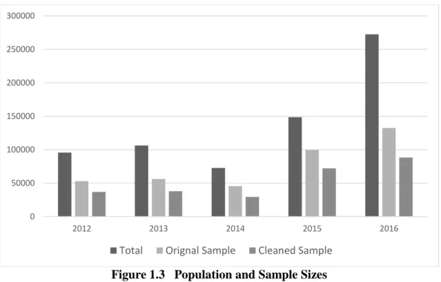
The original data set contains 386,790 transaction records from 2012-2016. After cleaning the data (such as missing values and outliers; see Appendix A for details), this paper keeps 262,533 observations for analysis. All observations in the data set are resale commodity housing units, which were built for sale at market prices (Fu et al., 2000). Figure 1.3 shows that our sample represents half of the total transactions in Beijing and the cleaned sample represents about one third.
Figure 1.3 Population and Sample Sizes 1.4.3 Variable
The descriptive statistics of all variables are shown in Table 1.1. The dependent variable is unit selling price (per square meter), which is the standard measure of housing prices in China15. All prices are in real term in 2009 RMB level. One feature of the Beijing housing
15 See examples in Hong Kong (Bao & Wan, 2004). 0 50000 100000 150000 200000 250000 300000 2012 2013 2014 2015 2016
29
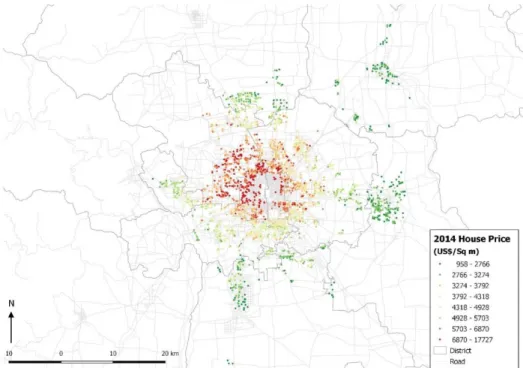
prices is the concentric pattern. See Figure 1.4-1.8 for the sample distribution across locations in Beijing from 2012 to 2016.
Figure 1.4 Beijing Resale Housing Price (2012 Sample)
30
Figure 1.6 Beijing Resale Housing Price (2014 Sample)
31
Figure 1.8 Beijing Resale Housing Price (2016 Sample)
The independent variables have four types: structural attributes, building-related attributes, time identifiers, and location identifiers.
Structural attributes contain the number of rooms, including bedrooms (BED), living rooms (LIV), and bathrooms (BATH). The signs of the estimated coefficients of these rooms are expected to be positive. However, the relationship between bedroom and price could be nonlinear. The size of the unit is measured by its floor area (FAREA). The sign of FAREA is uncertain from the literature. However, since this paper uses the unit price, the sign is more likely to be negative. Due to the data limitation, the floor level (FLVL) is in relative levels. There are five categories (1-5) to indicate whether a housing unit is located on the ground floor, low level, middle level, high level, or the top floor of a building respectively. Exposure to the south (SOUTH) is expected to have a positive effect. Averagely, 77% units have at least one window facing south. This percent is significant because not only right south but directions like southwest and southeast are also regarded
32
as an exposure to the south. Facing both south and north (SNEXP) is good for ventilation, which is considered as a premium in Beijing.
For building attributes, the total number of floors (TNFL) represents the height of the building. The effect of a high building is mixed with unexpected signs. Building types (BTYPE) include slab building, tower building and mixed building. Year built (BYEAR) is the year in which the building was completed. The age of buildings has a negative correlation with housing prices in most studies of MRMs (Mok et al., 1995; Bao & Wan, 2004; Jim & Chen, 2009; Jim & Chen, 2010; Shimizu et al., 2010). A negative effect but positive sign is expected. Elevator (ELEV) equals to one if the building is equipped with elevators. The elevator is important for high-rise buildings and thus should be positively correlated with prices. Interaction terms should also be considered. Heating system (HEAT) is available in the dataset. It equals one if there is a central heating system in the building and equals to zero if it is self-heating.
Table 1.1 Descriptive Statistics Variable Description Unit &
Type Mean St. d. Min Median Max
Dependent Variable
DTUP Deflated transaction unit price*
RMB/Square Meter
32564.9 14175.3 4954.5 29632.4 123902.29
Independent Variable
House-specific Structural Attributes
BED Number of bedrooms 1.97 0.71 1 2 5
LIV Number of living Rooms 1.18 0.50 0 1 2
BATH Number of bathrooms 1.16 0.38 0 1 3
FAREA Floor area Square
Meter
81.23 31.09 12.96 74.29 356
FLVL Floor Level; relative position in the building: 1—Ground Floor 2—Low Position 3—Middle Position 4—High Position 5—Top Floor Categorical (1-5) 3.10 1.09 1 3 5
33
is exposed to South: 0—No
1—Yes
SNEXP Whether the housing unit is exposed to both North and South:
0—No 1—Yes
Dummy 0.47 0.50 0 0 1
Building-related Structural Attributes
TNFL Total number of floors 13.30 7.83 2 11 40
BTYPE Building type: 1—Slab Building 2—Tower Building 3—Mixed Type Categorical (1-3) 1.63 0.78 1 1 3
BYEAR Year built 1999.37 8.24 1893 2001 2016
ELEV Whether equipped with elevator: 0—No 1—Yes Dummy 0.58 0.49 0 1 1 HEAT Heating: 0—Self Heating 1—Building Heating Dummy 0.85 0.35 0 1 1 Time Identifiers
TYEAR Transaction year Categorical
(2012-2016)
2014.51 1.43 2012 2015 2016
TMON Transaction month Categorical
(1-12)
6.61 3.35 1 7 12
Location Identifiers
LOC Location Categorical
*All prices are deflated into real prices in the year 2009 RMB. CPI indices are from China Statistical Yearbook 2011-2015 and other sources from the government.
1.4.4 Model Specification
This paper applies the hedonic price function in a linear semi-log form16: logged housing prices as the dependent variable and no transformation for the independent variables. Different specifications include different variables.
Temporal factors are incorporated as dummies of transaction years and months, or dummies of year-month interactions. The number of bedrooms is treated as in two ways: categorical and continuous. Another categorization is applied to the floor areas. Following
16 This paper tried Box-Cox transformation of the dependent variable. However, the likelihood-ratio tests
cannot reject lamda = 0, i.e., the log specification of the dependent variable. To focus on the comparison of FE and LNE, this paper applies the semi-log form for all models.
34
Gao and Asami (2011), this paper splits the floor area into 6 categories: [12, 40), [40, 50), [50, 60), [60, 80), [80, 190), and [190, 440). In addition, interactions among floor level, elevator, and building height are explored.
Note that for each model above, both FE and LNE are employed for estimation. Following the recommendation of Solon, Haider, & Wooldridge (2015), both FE (unweighted) and LNE (weighted) estimates and their cluster-robust standard errors (in parentheses) are reported.
1.4.5 Result
Comparing OLS, FE, and LNE
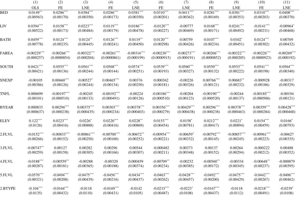
In Table 1.2, the left three columns show the comparison between OLS, FE, and LNE. Some location variables are added for OLS. FE and LNE have no estimates for these location variables but produce consistent estimates for others. Theoretically, FE and LNE should produce similar estimates since both are unbiased and consistent; and the cluster-robust standard errors of FE should be smaller than those of LNE since FE is asymptotically more efficient according to Chapter 2. This is exactly the case in Table 1.2. The estimates of FE are close to LNE but with smaller standard errors. In contrast, the estimates of OLS are very different, suggesting the biasedness from endogeneity issues.
35
Table 1.2 FE and LNE with Different Time Variables
(1) (2) (3) (4) (5) (6) (7) (8) (9) (10) (11)
OLS FE LNE FE LNE FE LNE FE LNE FE LNE
BED 0.0149** 0.0286*** 0.0384*** 0.0286*** 0.0381*** 0.0310*** 0.0411*** 0.0281*** 0.0381*** 0.0310*** 0.0408*** (0.00563) (0.00170) (0.00350) (0.00173) (0.00350) (0.00201) (0.00362) (0.00169) (0.00353) (0.00203) (0.00370) LIV 0.0394*** 0.0158*** 0.0223*** 0.0119*** 0.0186*** -0.0120*** -0.00777 0.0168*** 0.0241*** -0.0141*** -0.00964* (0.00522) (0.00173) (0.00484) (0.00179) (0.00478) (0.00227) (0.00469) (0.00171) (0.00492) (0.00231) (0.00468) BATH 0.0459*** 0.0124*** 0.0124** 0.0126*** 0.0119** 0.0120*** 0.00759 0.0107*** 0.0102* 0.0124*** 0.00769 (0.00778) (0.00235) (0.00445) (0.00241) (0.00450) (0.00298) (0.00426) (0.00234) (0.00451) (0.00302) (0.00432) FAREA -0.00229*** -0.00266*** -0.00322*** -0.00261*** -0.00316*** -0.00230*** -0.00273*** -0.00266*** -0.00322*** -0.00226*** -0.00269*** (0.000257) (0.0000854) (0.000204) (0.0000861) (0.000199) (0.0000915) (0.000191) (0.0000852) (0.000205) (0.0000923) (0.000192) SOUTH 0.0421*** 0.0555*** 0.0561*** 0.0568*** 0.0574*** 0.0539*** 0.0560*** 0.0550*** 0.0553*** 0.0541*** 0.0564*** (0.00421) (0.00136) (0.00244) (0.00144) (0.00251) (0.00193) (0.00327) (0.00132) (0.00222) (0.00198) (0.00340) SNEXP -0.00105 0.00660*** 0.00527* 0.00465*** 0.00376 0.000362 -0.00226 0.00766*** 0.00683** -0.000928 -0.00317 (0.00386) (0.00126) (0.00244) (0.00134) (0.00250) (0.00181) (0.00326) (0.00121) (0.00232) (0.00186) (0.00329) TNFL 0.000699 -0.00197*** -0.00245 -0.00192*** -0.00224 -0.00186*** -0.00204 -0.00190*** -0.00244 -0.00185*** -0.00194 (0.00101) (0.000510) (0.00133) (0.000491) (0.00126) (0.000510) (0.00123) (0.000520) (0.00137) (0.000506) (0.00121) BYEAR 0.000833 0.00296*** 0.00375*** 0.00303*** 0.00378*** 0.00356*** 0.00429*** 0.00296*** 0.00378*** 0.00359*** 0.00428*** (0.000637) (0.000238) (0.000435) (0.000234) (0.000403) (0.000279) (0.000438) (0.000238) (0.000463) (0.000284) (0.000460) ELEV 0.122*** 0.0223*** 0.0226* 0.0220*** 0.0228** 0.0153*** 0.0158* 0.0212*** 0.0221* 0.0154*** 0.0166* (0.0126) (0.00416) (0.00888) (0.00416) (0.00869) (0.00454) (0.00781) (0.00417) (0.00894) (0.00459) (0.00793) 2.FLVL -0.0152*** -0.00833*** -0.00861*** -0.00700*** -0.00672** -0.00954*** -0.00659* -0.00792*** -0.00857*** -0.00961*** -0.00627 (0.00266) (0.00152) (0.00250) (0.00160) (0.00252) (0.00221) (0.00332) (0.00145) (0.00245) (0.00223) (0.00335) 3.FLVL -0.00747** 0.00127 0.00282 0.00296 0.00544 -0.000482 0.00373 0.00137 0.00264 -0.000222 0.00488 (0.00259) (0.00158) (0.00305) (0.00166) (0.00307) (0.00211) (0.00348) (0.00152) (0.00294) (0.00212) (0.00352) 4.FLVL -0.0188*** -0.00559** -0.00288 -0.00320 0.000459 -0.00709** -0.00232 -0.00560** -0.00334 -0.00648** -0.000879 (0.00287) (0.00181) (0.00365) (0.00188) (0.00374) (0.00234) (0.00385) (0.00172) (0.00345) (0.00237) (0.00395) 5.FLVL -0.0570*** -0.0494*** -0.0475*** -0.0456*** -0.0434*** -0.0463*** -0.0428*** -0.0492*** -0.0475*** -0.0442*** -0.0406*** (0.00321) (0.00208) (0.00439) (0.00216) (0.00437) (0.00262) (0.00457) (0.00200) (0.00429) (0.00267) (0.00462) 2.BTYPE -0.104*** -0.0164*** -0.0118 -0.0169*** -0.0142 -0.0215*** -0.0223* -0.0167*** -0.0118 -0.0218*** -0.0239* (0.0135) (0.00432) (0.0110) (0.00431) (0.0105) (0.00487) (0.0108) (0.00437) (0.0112) (0.00491) (0.0108)
36 3.BTYPE -0.0446*** -0.0153*** -0.00960 -0.0163*** -0.0115 -0.0189*** -0.0162* -0.0146*** -0.00853 -0.0191*** -0.0176** (0.0116) (0.00318) (0.00604) (0.00323) (0.00588) (0.00418) (0.00645) (0.00318) (0.00611) (0.00422) (0.00653) HEAT 0.0521*** -0.00801 -0.00334 -0.00650 -0.00174 -0.00767 -0.0103 -0.00657 -0.000349 -0.00678 -0.00842 (0.0125) (0.0108) (0.0156) (0.0111) (0.0159) (0.0131) (0.0160) (0.0110) (0.0158) (0.0134) (0.0165) Locational Yes
TYEAR? Yes Yes Yes Yes Yes
TMON? Yes Yes Yes Yes Yes
TYEAR* TMON? Yes Yes N 262533 262533 262533 262533 262533 262533 262533 262533 262533 262533 262533 adj. R2 0.755 0.768 0.766 0.673 0.674 0.086 0.089 0.831 0.831 0.029 0.035 F 1446.4 3375.3 1845.9 3482.1 1765.3 464.5 342.0 2117.5 1805.6 132.7 60.46
Standard errors in parentheses
37
Year Dummies
For the year dummies, all three estimators produce similar results (see Table 1.3 and Figure 1.9). This is largely because the year factor is relatively independent and immune to the endogeneity issues. The year effect on housing prices is very large. Comparing to the year 2012, transactions in 2013 have on average 30% higher prices. Prices in 2014 fall a little bit but are still 27% higher than 2012. Prices in 2015 are at similar level with 2013. In 2016, the housing price almost doubles the level of 2013.
Table 1.3 Estimates of Year Dummies
(1) OLS (2) FE (3) LNE 2013.TYEAR 0.318*** 0.321*** 0.321*** (0.00232) (0.00150) (0.00270) 2014.TYEAR 0.278*** 0.265*** 0.267*** (0.00308) (0.00198) (0.00325) 2015.TYEAR 0.318*** 0.303*** 0.298*** (0.00314) (0.00230) (0.00412) 2016.TYEAR 0.606*** 0.602*** 0.602*** (0.00406) (0.00338) (0.00683) N 262533 262533 262533 adj. R2 0.755 0.768 0.766 F 1446.4 3375.3 1845.9 0 0.1 0.2 0.3 0.4 0.5 0.6 2012 2013 2014 2015 2016 OLS FE LNE
38
Figure 1.9 Estimates of Year Dummies
Model (4) to (11) in Table 1.2 use different specification of the time variables. Focusing on FE models. When the model excludes all temporal factors as in Model (10), only around 2.9% of the price variation is explained, which could be regarded as the explanatory power of the structural variables. When adding the month dummies (Model 6), the ratio increases to 8.6%; the difference 5.7% is the explanatory power of the month variable. When only adding the year dummies (Model 4), the ratio becomes 67.3%, which indicates a 64.4% of the variation is explained by the year changes. At last, the best model seems to be (8) which use the interaction between years and months. Note that the parameter estimates are stable across different model specifications.
Structural and Building Variables
According to the results of Model (2), for housing-specific variables, one more unit of bedrooms (BED), living rooms (LIV), and bathrooms (BATH) are associated with an increase in housing price per square meter by 2.86%, 1.58%, and 1.24%, respectively. The floor area (FAREA) is negatively associated with housing prices by 0.3%, which is a quite small magnitude as compared to other housing attributes and very similar to the findings of Mok et al. (1995) in Hong Kong.
In terms of the magnitude of the coefficients, the exposure to the south (SOUTH) is the most influential positive attributes by 5.5%. The effect of being exposed to both south and north (SNEXP) is positive but with a smaller value of 0.66%. There is a slight ground premium. Compared to the ground floor (FLVL), low-level position corresponds to a price depreciation by 0.83%, high position by 0.56%, and the top floor by 4.9%. The effect of the middle position is not significantly different from that of the ground floor.
39
For building-specific variables, the total number of floors (TNFL) have a slightly negative relationship to housing prices by 0.2%. The built year (BYEAR) effect is positive. Housing prices increase by 0.3% if a building is one year newer. Being equipped with elevators (ELEV) has a significantly positive effect by 2.2%. For building types (BTYPE), the slab building has a larger effect of 1.5% than the tower building and the mixed building. The heating type (HEAT) has no significant relationship with housing prices.
Floor Level, Total Floors, and Elevator
In Table 1.2, one striking finding is the ground floor premium, which means residents prefer the ground floor to all other levels. This is a huge contrast to many MRMs where people favor the top floors. This paper further investigates the interaction between floor levels, elevators, and total floors.
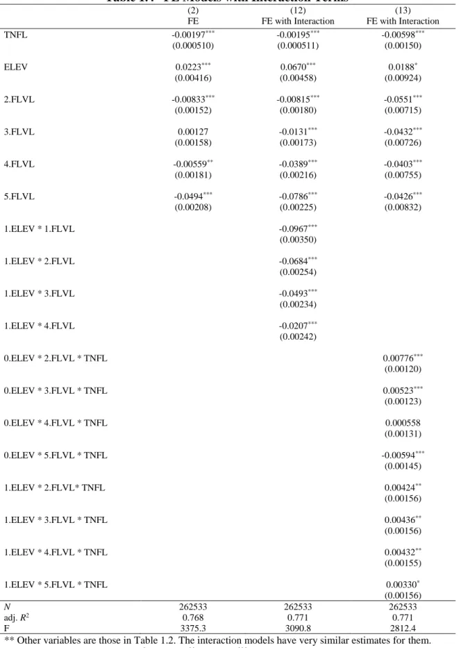
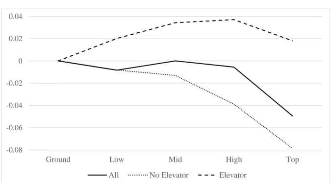
Table 1.4 shows the results of FE models with interaction terms. Model (12) includes the interaction term between the floor level and the elevator. Model (13) adds the total number of floors into the interaction. Most interactive terms have significant estimates. Floor level coefficients in different models are summarized in Table 1.5. The two columns of Model (12) in Table 1.5 and Figure 1.10 show that the ground premium found in model (2) gets larger when the building has no elevator but disappears for the buildings with elevators. In the latter case, the high position (not the top floor) is mostly favored. The columns of Model (13) and Figure 1.11 show that for buildings without elevators, the higher the building is, the less the top floor would be valued. In contrast, the low and middle positions are more valued with the building gets higher. For no-elevator buildings higher than 9 floors, both low and middle positions of the building are preferred
40
to the ground level. For buildings with elevators, as the total number of floors increases, the ground level premium decreases comparing to all other floor levels. When the total floor is larger than 13, all other floor levels are preferred to the ground one.
Analysis with interaction terms tells us that the ground level premium exists in Beijing for certain types of buildings. For no-elevator buildings less than 7 floors or with-elevator buildings less than 10 floors, the ground floor has the highest effects on housing prices. The ground level in a higher building is exposed to larger negative externality brought by the denser living environment.
41
Table 1.4 FE Models with Interaction Terms
(2) (12) (13)
FE FE with Interaction FE with Interaction
TNFL -0.00197*** -0.00195*** -0.00598*** (0.000510) (0.000511) (0.00150) ELEV 0.0223*** 0.0670*** 0.0188* (0.00416) (0.00458) (0.00924) 2.FLVL -0.00833*** -0.00815*** -0.0551*** (0.00152) (0.00180) (0.00715) 3.FLVL 0.00127 -0.0131*** -0.0432*** (0.00158) (0.00173) (0.00726) 4.FLVL -0.00559** -0.0389*** -0.0403*** (0.00181) (0.00216) (0.00755) 5.FLVL -0.0494*** -0.0786*** -0.0426*** (0.00208) (0.00225) (0.00832) 1.ELEV * 1.FLVL -0.0967*** (0.00350) 1.ELEV * 2.FLVL -0.0684*** (0.00254) 1.ELEV * 3.FLVL -0.0493*** (0.00234) 1.ELEV * 4.FLVL -0.0207*** (0.00242) 0.ELEV * 2.FLVL * TNFL 0.00776*** (0.00120) 0.ELEV * 3.FLVL * TNFL 0.00523*** (0.00123) 0.ELEV * 4.FLVL * TNFL 0.000558 (0.00131) 0.ELEV * 5.FLVL * TNFL -0.00594*** (0.00145) 1.ELEV * 2.FLVL* TNFL 0.00424** (0.00156) 1.ELEV * 3.FLVL * TNFL 0.00436** (0.00156) 1.ELEV * 4.FLVL * TNFL 0.00432** (0.00155) 1.ELEV * 5.FLVL * TNFL 0.00330* (0.00156) N 262533 262533 262533 adj. R2 0.768 0.771 0.771 F 3375.3 3090.8 2812.4
** Other variables are those in Table 1.2. The interaction models have very similar estimates for them. Standard errors in parentheses *p < 0.05, **p < 0.01, ***p < 0.001
42
Table 1.5 Interaction among Floor Level, Elevator, and Total Floor
(2) (12) (12) (13) (13)
Variable FE No Elevator Elevator No Elevator Elevator
Ground Floor 0 0 0 0 0
Low Position -0.00833 -0.00815 0.0201 -0.0551 +0.00776 * TNFL -0.0551 +0.00424 * TNFL Middle Position Not significant -0.0131 0.0343 -0.0432 +0.00523 * TNFL -0.0432 +0.00436 * TNFL
High Position -0.00559 -0.0389 0.0371 - 0.0403 -0.0403 + 0.00432 * TNFL
Top Floor -0.0494 -0.0786 0.0181 -0.0426 - 0.00594 * TNFL -0.0426 + 0.00330 * TNFL
Figure 0.10 Vertical Gradient (with and without Elevator) -0.08 -0.06 -0.04 -0.02 0 0.02 0.04
Ground Low Mid High Top
43
Figure 1.11 Vertical Gradient (with Elevator and Total Floors from 5 to 15)
8 9 10 11 12 13 14 15 5 6 7 -0.14 -0.105 -0.07 -0.035 0 0.035 0.07
Ground Low Mid High Top
With Elevator
8 9 10 11 12 13 14 15 6 7 5 -0.14 -0.105 -0.07 -0.035 0 0.035 0.07Ground Low Mid High Top
44
Categorical Bedroom Numbers and Floor Areas
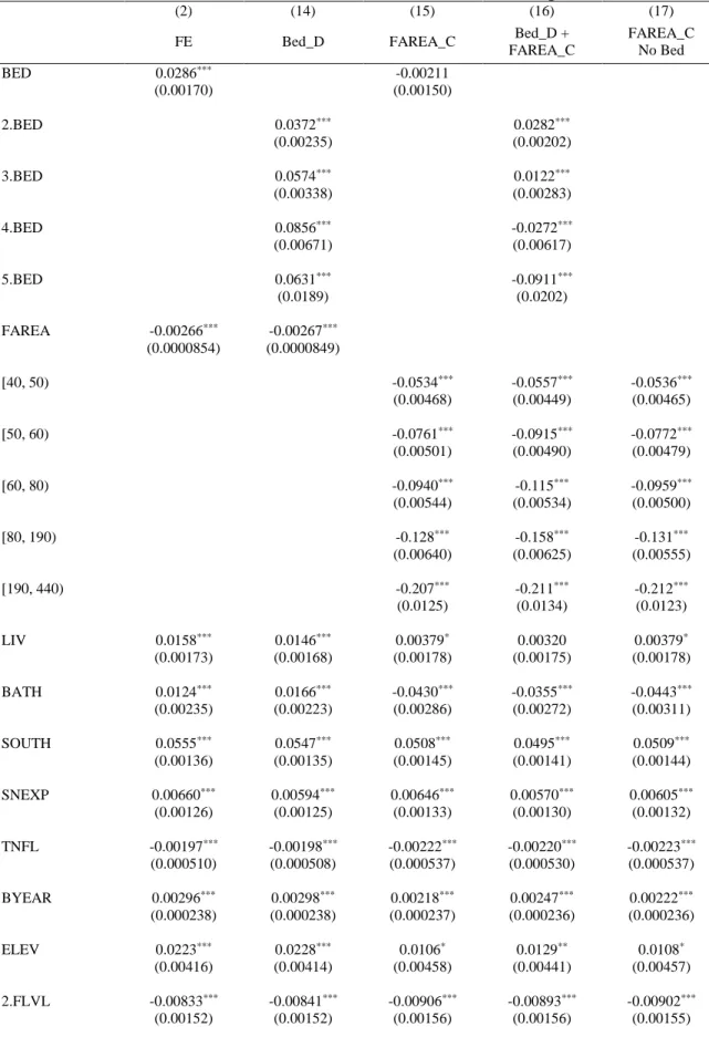
Lastly, this paper specifies the number of bedrooms as dummy variables and the floor area as a categorical variable. In Table 1.6, Model (2) is listed as a benchmark. Model (14) uses bedroom dummies, model (15) uses floor area categories, model (16) includes both, and model (17) excludes the variable of the bedroom from the regression. First, all other variables, except for other room numbers and the elevator, have stable parameter estimates across all specifications. Second, comparing model (14) and (16), the estimates of the bedroom dummies are inconsistent17. Without controlling for floor area categories (model 14), the 1-bedroom house is least favorable, and the 4-bedroom house has the largest effect on prices; while controlling for the floor area categories (model 16), the 2-bedroom house is the favorite, and houses with more bedrooms are less favored. Similar inconsistency can be found in models (2) and (15); the estimate of the original bedroom variable is affected and changes from positive to negative. In contrast, the floor area categories have more stable estimates. In model (17), when the variable of the bedroom is excluded from the regression, the results are still similar. Different from the findings from Gao and Asami (2011), who argues that [50, 60) and [80, 190) are more highly valued, this paper shows the smaller sizes are preferred.
17 This suggests a strong correlation between the number of bedroom and the floor area, which is in fact 0.7052.
45
Table 1.6 Bedroom Dummies and Floor Area Categories
(2) (14) (15) (16) (17)
FE Bed_D FAREA_C Bed_D +
FAREA_C FAREA_C No Bed BED 0.0286*** -0.00211 (0.00170) (0.00150) 2.BED 0.0372*** 0.0282*** (0.00235) (0.00202) 3.BED 0.0574*** 0.0122*** (0.00338) (0.00283) 4.BED 0.0856*** -0.0272*** (0.00671) (0.00617) 5.BED 0.0631*** -0.0911*** (0.0189) (0.0202) FAREA -0.00266*** -0.00267*** (0.0000854) (0.0000849) [40, 50) -0.0534*** -0.0557*** -0.0536*** (0.00468) (0.00449) (0.00465) [50, 60) -0.0761*** -0.0915*** -0.0772*** (0.00501) (0.00490) (0.00479) [60, 80) -0.0940*** -0.115*** -0.0959*** (0.00544) (0.00534) (0.00500) [80, 190) -0.128*** -0.158*** -0.131*** (0.00640) (0.00625) (0.00555) [190, 440) -0.207*** -0.211*** -0.212*** (0.0125) (0.0134) (0.0123) LIV 0.0158*** 0.0146*** 0.00379* 0.00320 0.00379* (0.00173) (0.00168) (0.00178) (0.00175) (0.00178) BATH 0.0124*** 0.0166*** -0.0430*** -0.0355*** -0.0443*** (0.00235) (0.00223) (0.00286) (0.00272) (0.00311) SOUTH 0.0555*** 0.0547*** 0.0508*** 0.0495*** 0.0509*** (0.00136) (0.00135) (0.00145) (0.00141) (0.00144) SNEXP 0.00660*** 0.00594*** 0.00646*** 0.00570*** 0.00605*** (0.00126) (0.00125) (0.00133) (0.00130) (0.00132) TNFL -0.00197*** -0.00198*** -0.00222*** -0.00220*** -0.00223*** (0.000510) (0.000508) (0.000537) (0.000530) (0.000537) BYEAR 0.00296*** 0.00298*** 0.00218*** 0.00247*** 0.00222*** (0.000238) (0.000238) (0.000237) (0.000236) (0.000236) ELEV 0.0223*** 0.0228*** 0.0106* 0.0129** 0.0108* (0.00416) (0.00414) (0.00458) (0.00441) (0.00457) 2.FLVL -0.00833*** -0.00841*** -0.00906*** -0.00893*** -0.00902*** (0.00152) (0.00152) (0.00156) (0.00156) (0.00155)
46 3.FLVL 0.00127 0.00117 0.000229 0.000341 0.000281 (0.00158) (0.00159) (0.00163) (0.00163) (0.00162) 4.FLVL -0.00559** -0.00563** -0.00651*** -0.00615*** -0.00648*** (0.00181) (0.00181) (0.00186) (0.00185) (0.00185) 5.FLVL -0.0494*** -0.0493*** -0.0500*** -0.0494*** -0.0500*** (0.00208) (0.00207) (0.00223) (0.00220) (0.00223) 2.BTYPE -0.0164*** -0.0167*** -0.00915 -0.00956* -0.00921 (0.00432) (0.00432) (0.00471) (0.00465) (0.00471) 3.BTYPE -0.0153*** -0.0153*** -0.0110** -0.0110** -0.0110** (0.00318) (0.00318) (0.00344) (0.00338) (0.00344) 2013.TYEAR 0.321*** 0.321*** 0.320*** 0.320*** 0.320*** (0.00150) (0.00151) (0.00152) (0.00152) (0.00152) 2014.TYEAR 0.265*** 0.265*** 0.265*** 0.265*** 0.265*** (0.00198) (0.00198) (0.00198) (0.00197) (0.00198) 2015.TYEAR 0.303*** 0.303*** 0.302*** 0.301*** 0.302*** (0.00230) (0.00230) (0.00230) (0.00230) (0.00231) 2016.TYEAR 0.602*** 0.602*** 0.601*** 0.600*** 0.601*** (0.00338) (0.00338) (0.00339) (0.00338) (0.00339) N 262533 262533 262533 262533 262533 adj. R2 0.768 0.769 0.758 0.760 0.758 F 3375.3 3098.9 2930.7 2774.7 3016.1
47
1.5 CONCLUSION AND DISCUSSION
This paper aims to explain the vertical variation in housing prices. The contribution of this paper is two-fold: empirical evidence and methodological exploration.
Empirically, this paper uses a large dataset of resale housing transaction records in Beijing from 2012 to 2016 and shows that temporal factors and the structural attributes together account for around 76% of the variation in housing prices. The structural attributes only account for about 3% of the variation; while the temporal factors, years and months, explain the rest 73%. The most important structural factor in Beijing is the exposure to the south, leading to around 5% increase in housing prices. Beijing features a ground floor premium, which is conditional on the building’s total number of floors and whether has an elevator. The floor areas are examined in both continuous and categorical terms. This small size preference contradicts the existing findings of Beijing housing markets in the literature.
Methodologically, this paper develops a least nugget effect estimator (LNE) which is equivalent to the pairwise differences estimator (PD) and generalizes the fixed effects estimator (FE) by weighting group sizes. This paper provides empirical evidence for the efficiency of FE over PD (and thus LNE) given large samples.
There are two limitations of this paper. The first is the assumption that there are no spatial and temporal dependencies of housing prices. This paper controls the within-group correlation by applying cluster-robust standard errors but at the same time assumes no between-group or inter-temporal dependencies. This may not be valid in housing markets where spatial and temporal autocorrelations widely exist. The fixed effects estimator has also been criticized for not fully controlling for spatial dependency (Anselin &
Arribas-48
Bel, 2013). Scholars have taken both spatial and temporal dependencies into consideration to control for the spatio-temporal autocorrelation effects in MRMs (Sun et al., 2005). The assumption may potentially bias the standard errors and the inference of the parameter estimates. The second limitation is to assume that the numbers of observations at each location are exogenous. This may not be valid since the unobservable characteristics of houses sold frequently could differ from those sold infrequently (Englund, Quigley, & Redfearn, 1999). The resultant selection bias might undermine the findings of this paper.