This work is distributed as a Discussion Paper by the
STANFORD INSTITUTE FOR ECONOMIC POLICY RESEARCH
SIEPR Discussion Paper No. 10-028
Selection on Moral Hazard in Health Insurance
by
Liran Einav
Amy Finkelstein
Stephen Ryan
Paul Schrimpf
Mark Cullen
Stanford Institute for Economic Policy Research
Stanford University
Stanford, CA 94305
(650) 725-1874
The Stanford Institute for Economic Policy Research at Stanford University supports research bearing on
economic and public policy issues. The SIEPR Discussion Paper Series reports on research and policy
analysis conducted by researchers affiliated with the Institute. Working papers in this series reflect the views
of the authors and not necessarily those of the Stanford Institute for Economic Policy Research or Stanford
University.
Selection on moral hazard in health insurance
Liran Einav, Amy Finkelstein, Stephen Ryan, Paul Schrimpf, and Mark Culleny April 2011
Abstract. In this paper we explore the possibility that individuals may select insurance coverage in part based on their anticipated behavioral response to the insurance contract. Such “selection on moral hazard” can have important implications for attempts to combat either selection or moral hazard. We explore these issues using individual-level panel data from a single …rm, which contain information about health insurance options, choices, and subsequent claims. To identify the behavioral response to health insurance coverage and the heterogeneity in it, we take advantage of a change in the health insurance options o¤ered to some, but not all of the …rm’s employees. We begin with descriptive evidence that is suggestive of both heterogeneous moral hazard as well as selection on it, with individuals who select more coverage also appearing to exhibit greater behavioral response to that coverage. To formalize this analysis and explore its implications, we develop and estimate a model of plan choice and medical utilization. The results from the modeling exercise echo the descriptive evidence, and allow for further explorations of the interaction between selection and moral hazard. For example, one implication of our estimates is that abstracting from selection on moral hazard could lead one to substantially over-estimate the spending reduction associated with introducing a high deductible health insurance option.
JEL classi…cation numbers: D12, D82, G22
Keywords: Insurance markets; Adverse selection; Moral hazard; Health insurance
We are grateful to Felicia Bayer, Brenda Barlek, Chance Cassidy, Fran Filpovits, Frank Patrick, and Mike Williams for innumerable conversations explaining the institutional environment of Alcoa, to Colleen Barry, Susan Busch, Linda Cantley, Deron Galusha, James Hill, Sally Vegso, and especially Marty Slade for providing and explain-ing the data, to Tatyana Deryugina, Sean Klein, Michael Powell, Iuliana Pascu, and James Wang for outstandexplain-ing research assistance, and to Ben Handel, Justine Hastings, Jim Heckman, Igal Hendel, Nathan Hendren, Kate Ho, Pat Kline, Jon Levin, Matt Notowidigdo, Phil Reny, Rob Townsend, and numerous seminar participants for helpful comments and suggestions. The data were provided as part of an ongoing service and research agreement between Alcoa, Inc. and Stanford, under which Stanford faculty, in collaboration with faculty and sta¤ at Yale University, perform jointly agreed-upon ongoing and ad hoc research projects on workers’ health, injury, disability, and health care, and Mark Cullen serves as Senior Medical Advisor for Alcoa, Inc. We gratefully acknowledge support from the NIA (R01 AG032449), the National Science Foundation Grant SES-0643037 (Einav), the Alfred P. Sloan Foundation (Finkelstein), the John D. and Catherine T. MacArthur Foundation Network on Socioeconomic Status and Health, and Alcoa, Inc. (Cullen), and the U.S. Social Security Administration through grant #5 RRC08098400-03-00 to the National Bureau of Economic Research as part of the SSA Retirement Research Consortium. Einav also acknowl-edges the hospitality of the Center for Advanced Study in the Behavioral Sciences at Stanford. The …ndings and conclusions expressed are solely those of the authors and do not represent the views of SSA, any agency of the Federal Government, or the NBER.
yEinav: Department of Economics, Stanford University, and NBER, leinav@stanford.edu; Finkelstein: Department
of Economics, MIT, and NBER, a…nk@mit.edu; Schrimpf: Department of Economics, MIT, paul_s@mit.edu; Ryan: Department of Economics, MIT, and NBER, sryan@mit.edu; Cullen: Department of Internal Medicine, School of Medicine, Stanford University, mrcullen@stanford.edu.
1
Introduction
Economic analysis of market failure in insurance markets tends to analyze selection and moral haz-ard as distinct phenomena. In this paper, we explore the potential for selection on moral hazhaz-ard in insurance markets. By this we mean the possibility that moral hazard e¤ects are heterogeneous across individuals, and that individuals’ selection of insurance coverage is a¤ected by their an-ticipated behavioral response to coverage – their “moral hazard type.” We examine these issues empirically in the context of employer-provided health insurance in the United States. Speci…cally, in addition to “traditional” selection based on one’s health risk, we also examine selection on the expected incremental medical spending due to insurance.
Such selection on moral hazard has implications for the standard analysis of both selection and moral hazard. For example, a standard – and ubiquitous – approach to mitigating selection in insurance markets is risk adjustment, i.e. pricing on observable characteristics that predict one’s insurance claims. However, the potential for selection on moral hazard suggests that monitoring techniques that are usually thought of as reducing moral hazard –such as cost sharing that varies across categories of claims with di¤erential scope for moral hazard – may also have important bene…ts in combatting adverse selection. In contrast, a standard approach to mitigating moral hazard is to o¤er plans with higher consumer cost sharing. But if individuals’anticipated behavioral response to coverage a¤ects their propensity to select such plans, the magnitude of the behavioral response could be much lower (or much higher) from what would be achieved if plan choices were unrelated to the behavioral response. As we discuss in more detail below, not only the existence of selection on moral hazard but also the sign of any relationship between anticipated behavioral response and demand for higher coverage is ex ante ambiguous. Ultimately, these are empirical questions. To our knowledge, however, there is no empirical work on selection on moral hazard in insurance markets.
Health insurance provides a particularly interesting setting in which to explore these issues. Both selection and moral hazard have been well-documented in the employer-provided health insurance market in the United States. Moreover, given the extensive government involvement in health insurance, as well as the concern about the size and rapid growth of the health care sector, there is considerable academic and public policy interest in how to mitigate both selection and moral hazard in this market.
Recognition of the possibility of selection on moral hazard, however, highlights potentially important limitations of analyzing these problems in isolation. For example, the sizable empirical literature on the likely spending reductions that could be achieved through higher consumer cost sharing has intentionally focused on isolating and exploring exogenous changes in cost sharing – such as those induced by the famous Rand experiment (Manning et al., 1987; Newhouse, 1993). Yet, the very same feature that solves the causal inference problem – namely randomization (or attempts to approximate it in the subsequent quasi-experimental literature on this topic) –removes the endogenous choice element. It thus abstracts, by design, from any selection on moral hazard, which could have important implications for the spending reductions achieved through o¤ering
plans with higher consumer cost sharing, especially since substantial plan choice is now the norm not only in private health insurance but also increasingly in public health insurance programs, such as Medicare Part D.
We explore these issues using data on the U.S. workers at Alcoa Inc., a large multinational pro-ducer of aluminum and related products. We observe individual-level data on the health insurance options, choices, and subsequent medical utilization of employees (and their dependents); we also observe relatively rich demographic information, including health risk scores. Crucially for iden-tifying and estimating moral hazard, we observe variation in the health insurance options o¤ered to di¤erent groups of workers. In an e¤ort to control health spending, Alcoa began introducing a new set of health insurance options in 2004, designed to encourage employees to move into plans with substantially higher consumer cost sharing. We calculate that, if there were no change in behavior, the move from the original options to the new options would have increased the average share of spending paid out of pocket from 13 to 28 percent. We exploit the fact that, for unionized employees, the introduction of the new health insurance options was phased in gradually, as the new health insurance options could only be introduced when existing union contracts expired.
We begin by providing descriptive and motivating evidence on moral hazard in our setting. Di¤erence-in-di¤erences estimates suggest that the new options are associated with an average reduction in total medical spending of about $600 (11 percent) per employee. We …nd evidence consistent with heterogeneity in this moral hazard e¤ect, such as larger spending reductions for older relative to younger employees, and for sicker relative to healthier employees. We also present suggestive evidence of selection on moral hazard, with those who initially selected more coverage appearing to have a greater behavioral response to a change in coverage.
In order to formalize the analysis of selection on moral hazard and to explore some of its implications, we develop a utility-maximizing model of individual health insurance plan choices and claims. This allows us to precisely de…ne “moral hazard” (a term whose usage is far from standardized in the literature) and, within the context of our model, identify selection on it. The model draws heavily on a relatively standard two-period framework for modeling health insurance demand and subsequent medical care utilization (as in, e.g., Cardon and Hendel, 2001). In the …rst period, a risk-averse expected-utility-maximizing individual makes optimal coverage choices based on his risk aversion, health expectations, and anticipated behavioral response to the contract choice. In the second period, health is realized and individuals make optimal medical expenditure decisions based on their realized health as well as on their chosen coverage. It is this last e¤ect which generates what we term moral hazard, with a larger responsiveness corresponding to a higher “moral hazard type.” We allow for unobserved heterogeneity along three dimensions: health expectations, risk aversion, and moral hazard, and for ‡exible correlation across these three.
An individual’s optimal health insurance choice involves a trade-o¤ of higher up-front premiums in exchange for lower ex-post out-of-pocket spending. All else equal, willingness to pay for coverage is increasing in the individual’s health expectation and his risk aversion; these are standard results. In addition, in our model, all else equal, willingness to pay for coverage is increasing in the individ-ual’s moral hazard type: individuals with a greater behavioral response to coverage bene…t more
from more coverage, since they will consume more care as a result. This is the “selection on moral hazard”comparative static that is the focus of our paper. Empirically, however, the sign (let alone the magnitude) of any selection on moral hazard is ambiguous and depends on the heterogeneity in moral hazard as well as the correlation between moral hazard type and the other primitives that a¤ect health insurance choice, expected health and risk aversion.
We use this model, together with the data on individual plan options, plan choice, and subse-quent medical spending, to recover the joint distribution of individuals’(unobserved) health type, risk aversion, and moral hazard type. The econometric model and its identi…cation share many properties with some of our earlier work on insurance (Cohen and Einav, 2007; Einav, Finkelstein, and Schrimpf, 2010). The inclusion of moral hazard and heterogeneity in it is new. The panel structure of the data and the staggered timing of the introduction of the new coverage options are key in allowing us to identify this new element. The model is estimated using Markov Chain Monte Carlo Gibbs sampler, and its …t appears reasonable.
Qualitatively, the model’s results are consistent with the descriptive evidence of selection on moral hazard. We …nd that individuals who exhibit a greater behavioral response to coverage are more likely to choose higher coverage plans. Quantitatively, we estimate substantial heterogeneity in moral hazard and selection on it. We focus on the counterfactual of moving from the most comprehensive to the least comprehensive of the new options –essentially moving them from a no deductible plan to a high ($3,000 for family coverage) deductible plan. In terms of heterogeneity in moral hazard, we …nd that the standard deviation across individuals of the spending reduction that would be achieved by this change in plans is more than twice the average. In terms of selection on moral hazard, we …nd that for determining the choice between these two plans, selection on moral hazard is roughly as important as “traditional” selection on health risk, and considerably more important than selection on risk aversion.
We use the model to examine some of the implications of the selection on moral hazard we detect for spending and for welfare. In terms of spending, our results suggest that if we were to introduce the high deductible plan in a setting where previously there was only the no deductible option, and price it so that 10 percent of the population chooses the high deductible plan, spending for those who choose the high deductible plan would fall by approximately $130 per person. By contrast, were we to ignore selection on moral hazard and assume that the 10 percent who chose the high deductible plan were randomly drawn, we would have estimated a spending reduction for those moved to the high deductible plan more than 2.5 times as large, at about $350 per person. In terms of welfare, we estimate that about two-thirds of the welfare gain that can be achieved in our setting by perfect risk adjustment that eliminates adverse selection could be achieved if better monitoring technologies eliminated selection on moral hazard. While our quantitative estimates are speci…c to our setting and our modeling choices, they nonetheless provide an interesting example of the potential for selection on moral hazard to play a non-trivial role in the analysis of both selection and moral hazard.
Our paper is related to several distinct literatures. As previously noted, our modeling approach is closely related to that of Cardon and Hendel (2001), which is also the approach taken by Bajari
et al. (2010), Carlin and Town (2010), and Handel (2010) in modeling health insurance plan choice. Like us, all of these papers have allowed for selection based on expected health risk. Our paper di¤ers in our focus on identifying and estimating moral hazard – and in particular heterogeneous moral hazard –and in examining the relationship between moral hazard type and plan choice. From a methodological perspective, we also di¤er from these and many other discrete choice models in that we do not allow for a choice-speci…c, i.i.d. error term, which does not seem appealing given the vertically rankable nature of our choices.
Our analysis of the spending reduction associated with changes in cost sharing is related to a sizable experimental and quasi-experimental literature in health economics analyzing the impact of higher consumer cost sharing on spending. The di¤erence-in-di¤erences exercises with which we begin our analysis is very much in the spirit of this literature, which searches for identifying variation in consumer health plans to isolate the causal impact of consumer cost sharing on health spending. Our central di¤erence-in-di¤erences estimate translates into an implied arc elasticity of medical spending with respect to the average out-of-pocket cost share of about -0.14. This is broadly similar to the …ndings of the existing experimental and quasi-experimental literature, which tends to produce arc elasticities in the range of -0.1 to -0.4, with the “central”Rand elasticity estimate of -0.2 (see Chandra, Gruber, and McKnight (2010) for a recent review). However, our subsequent exploration of heterogeneity in this average moral hazard e¤ect and selection on it suggests the need for caution in using such estimates, which do not account for endogenous plan selection, for forecasting the likely spending e¤ects of introducing the option of plans with higher consumer cost sharing. It also suggests that one can embed the basic identi…cation approach of the di¤erence-in-di¤erences framework in a model that allows for and investigates such endogenous selection.
Our examination of selection on moral hazard is motivated in part by the growing empirical liter-ature demonstrating that selection in insurance markets often occurs on dimensions other than risk. This literature has tended to abstract from moral hazard, and focused on selection on preferences, such as risk aversion (Finkelstein and McGarry, 2006; Cohen and Einav, 2007), cognition (Fang, Keane, and Silverman, 2008), or desire for wealth after death (Einav, Finkelstein, and Schrimpf, 2010). Our exploration of selection on moral hazard highlights another potential dimension of se-lection and one that, we believe, has particularly interesting implications for contract design (in contexts where moral hazard is important). For many questions the extent to which selection occurs on the basis of expected health type or risk aversion does not matter (see, e.g., Einav, Finkelstein, and Cullen, 2010). However, as we illustrate in this paper, for questions regarding the design of contracts to reduce selection and the implications of contract design for spending, the extent to which selection is based on moral hazard can be important.
Despite its potential importance, we are not aware of any empirical work attempting to identify and analyze selection on moral hazard in insurance markets.1 The basic idea of selection on moral
hazard, however, is not unique to us. Similar ideas have appeared in several other contexts. For
1
Karlan and Zinman (2009) observe that selection in a credit market may be on unobserved risk and/or on anticipated e¤ort, although they do not empirically distinguish between the two.
example, in the context of appliance choices and phone plan choices, respectively, Dubin and McFadden (1984) and Miravete (2003) estimate models in which the choice is allowed to depend on subsequent utilization, which in turn may respond to the utilization price. One general way to think about the concept of selection on moral hazard is in the context of estimating a treatment e¤ect of insurance coverage on medical expenditure. Within such a framework, selection on health risk would be equivalent to heterogeneity in (and selection on) the level (or constant term in a regression of medical spending on insurance coverage), while selection on moral hazard can be thought of as heterogeneity in (and selection on) the slope coe¢ cient. Indeed, Heckman, Urzua and Vytlacil (2006) present an econometric examination of the properties of IV estimators when individuals select into treatment in part based on their anticipated response to the treatment, a phenomenon they refer to as “essential heterogeneity.” They subsequently apply these ideas in the context of the returns to education in Carneiro, Heckman, and Vytlacil (2010).
The rest of the paper proceeds as follows. Section 2 describes the data and Section 3 presents descriptive evidence of moral hazard, heterogeneity in moral hazard, and selection on it in our data. Section 4 develops a two-period model of an individual’s health insurance plan choice and spending decisions. Building on this model, Section 5 presents the econometric speci…cation and describes its identi…cation and estimation, and Section 6 presents our results, as well as illustrates some of their implications for spending and welfare. The last section concludes.
2
Setting and Data
We study health insurance choices and medical care utilization of the U.S.-based workers (and their dependents) at Alcoa, Inc., a large multinational producer of aluminum and related products. Our main analysis is based on data from 2003 and 2004, although for some of the analyses we extend the sample through 2006.
In 2004, in an e¤ort to control health care spending by encouraging employees to move into plans with substantially higher consumer cost sharing, Alcoa introduced a new set of health insurance PPO options. The new options were introduced gradually to di¤erent employees based on their union a¢ liation, since new bene…ts could only be introduced when an existing union contract expired. The staggered timing in the transition from one set of insurance options to another provides a plausibly exogenous source of variation that can help us identify the impact of health insurance on medical care utilization, which is what we mean throughout by the term “moral hazard.”
Our data contain the menu of health insurance options available to each employee, the em-ployee’s coverage choices, and detailed, claim-level information on his (and any covered depen-dents’) medical care utilization and expenditures for the year.2 The data also contain relatively rich demographic information (compared to typical claims data), including the employee’s union a¢ liation, employment type (hourly or salary), age, race, gender, annual earnings, job tenure at
2Health insurance choices are made in November, during the open enrollment period, and apply for the subsequent calendar year. They can be changed during the year only if the employee has a qualifying event, which is not common.
the company, and the number and ages of other insured family members. In addition, we obtained a summary proxy of an individual’s health based on software that predicts future medical spending on the basis of previous years’detailed medical diagnoses and claims, as well as basic demographics (age and gender); importantly for our purposes, this generated “health risk score”is not a function of the individual’s coverage choice.3
Sample de…nition and demographics Alcoa has about 45,000 active employees per year. We
exclude about 15 percent of the sample whose data are not suited to our analytical framework.4 Given the source of variation used to identify moral hazard, we concentrate on the approximately one third of Alcoa workers who are unionized.5 We further exclude the approximately two thirds
of unionized workers that are covered by the Master Steel Workers’ agreement. These workers faced only one PPO option which was left unchanged over our sample period. Finally, we exclude the approximately 10 percent of unionized employees who choose HMOs or who opt out of Alcoa-provided insurance, thus limiting our sample to employees enrolled in one of Alcoa’s PPO plans.6
Our baseline sample therefore consists of the approximately 4,000 unionized workers (each year) not covered by the Master agreement. These workers belong to one of 28 di¤erent unions. Table 1 (top row) provides some descriptive statistics on the demographic characteristics of our baseline sample in 2003. Our sample is 72 percent white, 84 percent male, with an average age of 41, average annual income of about $31,000, and an average tenure of about 10 years at the company. Approximately one quarter of the sample has single (employee only) coverage, while the rest also cover additional dependents. The health risk score is calibrated to be interpreted as predicted medical spending relative to a randomly drawn person under 65 in the nationally representative population; Table 1 indicates that, on average, individuals in our sample have predicted medical spending that is about 5 percent lower than this benchmark.
The remaining rows of Table 1 show summary statistics for four di¤erent groups of employees
3This is a relatively sophisticated way of predicting medical spending as it takes into account the di¤erential persistence of di¤erent types of medical claims (e.g., diabetes vs. car accident) in addition to overall utilization, demographics, and a rich set of interactions among these measures. The particular software we use is a risk adjustment tool called DXCG risk solution which was developed byVerisk Health and is used by, among other organizations, the Center for Medicare and Medicaid services in determining reimbursement rates in Medicare Advantage. See Bundorf, Levin, and Mahoney (2009), Carlin and Town (2010), and Handel (2010) for other examples of academic uses of this type of predictive diagnostic software.
4
The biggest reduction in sample size comes from excluding workers who are not at the company for the entire year (for whom we do not observe complete annual medical expenditures). In addition, we exclude employees who are outside the traditional bene…t structure of the company (for example because they were working for a recently acquired company with a di¤erent (grandfathered) bene…t structure); for such employees we do not have detailed information on their insurance options and choices. We also exclude a small number of employees because of missing data or data discrepancies.
5
Approximately 70 percent of Alcoa workers are hourly employees, and approximately half of these are unionized. Salaried workers are not unionized.
6As is typical in claims data sets, we lack information for employees who choose an HMO or who opt out of employer coverage on both the details of their insurance coverage and their medical care utilization. Of course, this raises potential sample selection concerns. Reassuringly, as we show in Appendix A, the change in PPO health insurance options does not appear to be associated with a statistically or economically signi…cant change in the fraction of employees who choose one of these excluded options.
based on when they were switched to the new bene…t options (i.e. four di¤erent treatment groups); we discuss this comparison when we present our di¤erence-in-di¤erences strategy and results below. As noted, our main analysis is based on the 2003 and 2004 data (7,570 employee-years and 4,477 unique employees). We exclude the 2005 and 2006 data from our primary analysis because it introduces two challenges for estimation of our plan choice model. First, the relative price of comprehensive coverage on the new options was raised substantially in 2005 and raised further in 2006, yet remarkably few employees already in the new option set changed their plans. This is consistent with substantial evidence of inertial behavior in health insurance plan choices (Handel, 2010; Carlin and Town, 2010). Rather than modeling this behavior (e.g., as switching costs), we prefer instead to restrict the data to a time period where they are less central to understanding plan choices. Of course, plan choice for individuals under the old options may also re‡ect inertial factors (indeed, as we will show in Table 3 below, plan switching is extremely rare (about 1 percent) for employees whose options did not change in 2004), but the pricing under the old options is not changing during our sample period, making any such inertia less central for trying to understand current choices. Second, the pricing in 2006 is such that it is hard to rationalize some of the plan choices in which there is considerable mass, without extending the model to include some combination of switching costs, additional plan features, and/or biased expectations; again, we prefer to avoid these issues in the context of our primary question of interest.
The main drawback to limiting the data to 2003 and 2004 is that less than one-…fth of our sample were o¤ered the new bene…ts starting in 2004, while another half of the sample was transitioned to the new bene…ts in 2005 and 2006 (Table 1, column (1)). Therefore, for some of the descriptive evidence we report in this section (which does not require an explicit model of plan choice) we use data from 2006. This sample produces qualitatively similar descriptive results to the 2003-2004 sample, but the larger sample size allows for greater precision (and hence probing) in our descriptive exercises.
Medical spending We have detailed, claim-level information on medical expenditures and
uti-lization. Our primary use of these data is to construct annual total medical spending for each employee (and his covered dependents). In Appendix A, we also use these data in a less aggregated way to break out spending by category (i.e., doctor’s o¢ ce, outpatient, inpatient, and other).
Figure 1 graphs the distribution of medical spending for our sample. We show the distribution separately for the approximately three-quarters of our sample with non-single coverage and the remainder with single employee coverage; not surprisingly, average spending is substantially higher in the former group. Across all employees, the average annual spending (on themselves and their covered dependents) is about $5,200.7 As is typical, medical expenditures are extremely skewed. For example, for non-single coverage, average spending ($6,100) is about 2.5 times greater than the median spending ($2,400), about 4 percent of our baseline sample has no spending, while each of
7
A little over one quarter of total spending is in doctor o¢ ces, about one third is for inpatient hospitalizations, and about one third is for outpatient services. About half of the remaining four percent of spending is accounted for by emergency room visits.
the employees in the top decile spends over $13,000.
Health insurance options and choices An attractive feature of our setting is that the PPO
plans in both the original and new regimes di¤er (within and across regimes) only in their consumer cost sharing requirements. They are identical on all non-cost sharing features, such as the network de…nition. Table 2 summarizes the original and new plan options and the fraction of employees who choose each option in our baseline sample. Employees may choose from up to four coverage tiers: single (employee only) coverage, or one of three non-single coverage tiers (employee plus spouse, employee plus children, or family). In our analysis we take coverage tier as given, assuming that it is primarily driven by family structure.8
There were three PPO options under the old bene…ts and …ve entirely di¤erent PPO options under the new bene…ts. Because there was no option of “staying in your existing plan”–the …ve new options were all distinct from the three old options in both their name and their design –individuals did not have the option of passively being defaulted into their existing coverage. We show in Table 3 below that plan choices for those who are switched to the new options are also consistent with the notion of “active”choices. As a result, we suspect that defaults did not play an important role in the choice of new bene…ts. Indeed, although option 4 was the default coverage option, it was not the most common choice (Table 2).9 In the robustness section we provide additional analysis that
suggests that the importance of defaults for our analysis is negligible.
The primary change from the old to the new bene…ts was to o¤er plans with higher deductibles and to increase the lowest out-of-pocket maximum.10 As shown in the table, under the new options there was a shift to plans with higher consumer cost sharing. Under the old options virtually all employees faced no deductible. Looking at employees with non-single coverage in Panel B (patterns for single coverage employees are similar), about two …fths faced a $2,000 out-of-pocket maximum while three-…fths faced a $5,000 out-of-pocket maximum. By contrast, under the new options, about a third of the employees faced a deductible, and all of them faced a high out-of-pocket maximum of at least $5,000 for non-single coverage.11
8Employee premiums vary across the four coverage tiers according to …xed ratios. Cost sharing provisions di¤er only between single and non-single coverage. Speci…cally, for a given PPO, deductibles and out-of-pocket maxima are twice as great for any non-single coverage tier as they are for single coverage. As shown in Table 1, about one quarter of the sample chooses single coverage. Within non-single coverage, slightly over half choose family coverage, 30 percent choose employee plus spouse, and about 16 percent choose employee plus children (not shown).
9
Also consistent with a large amount of “active” choices, although the old option 2 and the new option 5 are identical in all the aspects we model, only about half the employees who chose the old option 2 choose the new option 5, presumably re‡ecting the change in choice set (including relative pricing).
1 0At a point in time, prices within a coverage tier vary slightly across employees (in the range of several hundred dollars) under either the old or new options, depending on the employee’s a¢ liation (see Einav, Finkelstein, and Cullen (2010) for more detail). Premiums were constant over time under the old options; as mentioned, under the new options, premiums were increased substantially (and cross-employee di¤erences were removed) in 2005 and 2006 (not shown).
1 1A $5,000 ($2,500) out-of-pocket maximum for non-single (single) coverage is rarely binding. With no deductible and a 10 percent consumer cost sharing, the employee must have $50,000 ($25,000) in total annual medical expen-ditures to hit this out-of-pocket maximum. Using the realized claims, we calculate that only about one percent of the employees would hit the out-of-pocket maximum in a given year. By contrast, under the old options the lowest
As one way to summarize the di¤erences in consumer cost sharing under the di¤erent plans, we used the plan rules to simulate the average share of medical spending that would be paid out of pocket (counterfactually for most individuals) under di¤erent plans for all 2003 employees and their realized medical claims.12 Less generous plans correspond to those with higher consumer cost sharing. The results are summarized in the third row of each panel of Table 2. Combining the information on average enrollment shares of the di¤erent plans with our calculation of the average cost sharing in the di¤erent plans, we estimate that, holding spending behavior constant, the change from the original options to the new options on average would have more than doubled the share of spending paid out of pocket, from about 13 to 28 percent.13
The plan descriptions in Table 2, and the subsequent parameterization of our model in Section 5, abstract from some additional details. First, while we model all plans as having a 10 percent in-network consumer coinsurance after the plan deductible is reached for all care, under the old options doctor visits and ER visits had in fact co-pays rather than coinsurance.14 Second, we have summarized (and modeled) the in-network features only. All of the plans have higher (less generous) consumer cost sharing for care consumed out of network rather than in network. We choose to model only the in-network rules (where more than 95% of spending occurs) in order to avoid having to model the decision to go in or out of network. Third, while in general the new options were designed to have higher consumer cost sharing, a wider set of preventive care services (including regular physicals, screenings, and well baby care) were covered with no consumer cost sharing under the new options; these preventive services account for less than 2 percent of medical spending in our sample. Finally, the least comprehensive of the new options (option 1) includes a health reimbursement account (HRA) into which the employer makes tax-free contributions that the employee can draw on to pay for out-of-pocket medical expenses, or roll over for subsequent years. In the robustness section we explore alternative models that try to account for these distinctive features of this option.
Table 3 shows plan transitions for employees who were in the old options in both 2003 and 2004 and for employees who were switched from the old to the new options in 2004. Two main features emerge. First, almost all employees (almost 99 percent) under the old options in both years maintain the same coverage, which is to be expected given that the options and their prices did not change (but could also be driven by inertia in plan choices). Second, for those who get
out-of-pocket maximum was $2,000 ($1,000) for non-single (single) coverage, corresponding to total annual spending of $20,000 ($10,000). Using the same realized claims distribution, we calculate that about 5.5 percent of employees would hit this out-of-pocket maximum.
1 2By constructing (counterfactually) the share of a given (constant) set of medical expenditures that would be covered by di¤erent plans, we are able to construct a measure of the relative comprehensiveness of di¤erent plans that is purged of the confounding factors of selection and moral hazard that in‡uence the actual out-of-pocket share of medical expenditures covered by each plan.
1 3
These numbers are based on the average out of pocket shares by plan calculated in Table 2 and the plan shares for the 2003-2006 sample (not shown). Using the 2003-2004 sample’s plan shares (shown in Table 2) we estimate that the move to the new options would on average raise the average out of pocket share from 12 to 25 percent.
1 4Speci…cally they had doctor and ER co-pays of $15 and $75 respectively, or $10 and $50 depending on the plan. In practice, given the average costs of a doctor visit ($115) and an ER visit ($730) in our data, the switch from the co-pay to coinsurance did not make much di¤erence for predicted out-of-pocket spending.
switched to the new options in 2004, there is far from a perfect correlation in the rank ordering of their choices under the old and new options. Over 40 percent of individuals move from the highest possible coverage under the old option to something other than the highest possible coverage under the new options, or vice versa. This is consistent with individuals making more “active” choices under the new options, as suggested earlier.
3
Descriptive Evidence of Moral Hazard
We start by presenting some basic descriptive evidence of moral hazard in our setting. The analysis provides a feel for the basic identi…cation strategy for moral hazard. It also provides suggestive evidence of heterogeneity in moral hazard and selection on it. At the same time, our descriptive exercise points to the di¢ culty in identifying heterogeneity in moral hazard and selection on it without a formal model of moral hazard. The suggestive evidence as well as its important limitations together motivate our subsequent modeling exercise, which we turn to in the next section.
Descriptive estimates of moral hazard We start with the (easier) empirical task of
document-ing the existence of some form of asymmetric information in our data. Table 4 reports realized medical spending as a function of insurance coverage in our baseline sample. The analysis –which is in the spirit of Chiappori and Salanie’s (2000) “positive correlation test” – shows that under either the old or new options individuals who choose more comprehensive coverage have systemati-cally higher (contemporaneous) spending. This is consistent with the presence of adverse selection and/or moral hazard in our data.
To identify moral hazard in the data separately from adverse selection, we take advantage of the variation in the option set faced by di¤erent groups of employees. Table 5 presents this basic di¤erence-in-di¤erences evidence of moral hazard for our baseline sample. Speci…cally, we show various moments of the spending distribution in 2003 and in 2004 for the control group (employees who are covered by the old options in both years) and the treatment group (employees who are switched to the new options in 2004). The results show a strikingly consistent pattern across all the various moments of the spending distribution: spending falls for the treatment group, and tends to increase slightly for the control group.
The results in Table 5 also suggest slight di¤erences in 2003 spending for the treatment group relative to the control group, although these cross-sectional di¤erences are, for the most part, small relative to the changes over time within the treatment group. More generally, the bottom four rows of Table 1 indicate di¤erences in demographics as well as initial spending across all four of the treatment groups. In Appendix A we therefore explore in depth the sensitivity of our di¤erence-in-di¤erences estimates to controlling for observable di¤erence-in-di¤erences across employees. We also investigate in the Appendix the validity of the underlying identifying assumption behind the di¤erence-in-di¤erences estimates, namely that absent the changes in health insurance bene…ts these di¤erent groups would have experienced similar trends in health spending. We …nd these results generally quite reassuring.
Table 6 summarizes our central di¤erence-in-di¤erences estimates (which we then explore in more detail in Appendix A). Columns (1)-(3) show the results for our baseline 2003-2004 sample. The …rst column shows the di¤erence-in-di¤erences estimate when the dependent variable is mea-sured in dollars. Such a speci…cation assumes that the moral hazard e¤ects of insurance occurs in levels. This is consistent with the model we write down in the next section. However, both because it is possible that the moral hazard e¤ect is in fact proportional to spending, and because one may be concerned about the results being driven by a few outliers with extremely high spending, in columns (2) and (3) we investigate speci…cations that give rise to a proportional moral hazard e¤ect. Given the large fraction of employees with zero spending, we cannot estimate the model in simple logs. Instead, in column (2) we report estimates from a speci…cation in which spending,m, is measured bylog(1 +m),15 and column (3) reports a quasi-maximum likelihood Poisson model.16 The results suggest that the move to the new options is associated with an economically signi…cant decline in spending.
An important concern about the results in columns (1)-(3) is that they are not very precise. This is re‡ected in the large standard errors of the estimate, and in the relatively large di¤erences in the quantitative implications of the di¤erent speci…cations. This lack of precision is driven by the fact that only about one-…fth of the employees in our sample are switched to the new bene…ts in 2004 (Table 1, column (1)). Therefore, in columns (4)-(6) we report analogous estimates from the 2003-2006 sample, during which more than half of the employees switched to the new bene…ts. As expected, the standard error of our estimates decreases substantially, and the quantitative implications of the results become much more stable across speci…cations. The estimated spending reduction is now statistically signi…cant at the 5 percent level, with the point estimates suggesting a reduction of spending of about $600 (column (4)) or 11-17% (columns (5) and (6)). In Appendix A we show that the reduction in spending appears to arise entirely through reduced doctor and outpatient spending, with no evidence of a discernible e¤ect on inpatient spending.17
Following common practice in this literature, we can compute a back-of-the-envelope elasticity of health spending with respect to the out-of-pocket cost sharing by combining these estimates of the spending reduction with the estimates in Table 2 of the average cost sharing of di¤erent plans (holding behavior constant). Given the distribution of employees across the di¤erent plans, the numbers in Table 2 suggest that the change from the old options to the new options should increase the average share of out-of-pocket spending from 12.6 percent to 28.4 percent in the 2003-2006 sample. Combining the point estimate of a $591 reduction in spending (Table 6, column (4)) with our calculation of the increase in cost sharing, our estimates imply an arc elasticity of medical
1 5
Given that almost all individuals spend at least several hundred dollars (Figure 1), the results are not sensitive to the choice of 1 relative to some other small numbers. For the same reason, the estimated coe¢ cients can be approximately interpreted as elasticities.
1 6
The QMLE-Poisson model requires only that the conditional mean be correctly speci…ed for the estimates to be consistent. See, e.g., Wooldridge (2002, Chapter 19) for more discussion.
1 7
The reduction in outpatient spending appears to occur entirely on the intensive margin, while the reduction in doctor spending may occur entirely through a reduction in doctor visits.
spending with respect to out-of-pocket cost sharing of about -0.14.18 This is broadly similar to
the widely used Rand experiment arc-elasticity of medical spending of -0.2 (Manning et al., 1987; Keeler and Rolph, 1988). Subsequent studies that have used quasi-experimental variation in health insurance plans have tended to estimate elasticities of medical spending in the range of -0.1 to -0.4.19
Heterogeneity in moral hazard A necessary (but not su¢ cient) condition for selection on
moral hazard is that there is heterogeneity in individuals’ responsiveness to consumer cost shar-ing. To our knowledge, the experimental and quasi-experimental literature in health economics analyzing the impact of higher consumer cost sharing on spending has focused on average e¤ects and largely ignored potential heterogeneity. This may in part re‡ect the fact that because health realizations are, by their nature, partially random, testing for heterogeneity in moral hazard is not trivial. It is particularly challenging without an explicit model of the nature of moral hazard which can, for example, provide guidance as to whether the e¤ect of consumer cost sharing is ad-ditive or multiplicative.20 In addition, because changes in health insurance change the consumer’s (non-linear) budget set and individuals will vary as to where on the budget set they are, a careful examination of heterogeneity in moral hazard involves modeling this heterogeneity in the “treat-ment” associated with a change in health insurance plan; see Einav and Finkelstein (2011) for an exploration of related issues. In our speci…c context, a further subtlety is that it is the menu of plan options that varies in a quasi-experimental fashion, rather than the plan itself, making the actual individual coverage endogenous. All of these considerations motivate our formal modeling of moral hazard and of plan choice in the next section.
We begin, however, by …rst presenting some suggestive evidence in the data of what might plausibly be heterogeneity in moral hazard. One approach is to look at the distribution of spending changes across individuals. In the context of a model with an additive separable moral hazard e¤ect (such as the one we develop in the next section), homogeneous moral hazard would imply a constant (additive) change in spending for all individuals. The results in Table 5 showing the di¤erence-in-di¤erences estimates at di¤erent quantiles of the distribution indicate that the change in spending associated with the change in insurance options is higher at higher quantiles. Due to
1 8
We compute an arc elasticity, in which the proportional change in spending (and in consumer cost sharing) is calculated relative to the average observed across the old and new options, so that our results are more directly comparable with the existing literature. The arc elasticity is calculated as (q2 q1)=(q1+q2)=2
(p2 p1)=(p1+p2)=2 where p denotes the
average consumer cost sharing rate. For the 2003-2006 sample, the proportional change in spending and cost sharing is 11% and 77%, respectively.
1 9
See Chandra, Gruber, and McKnight (2010), who provide a recent review of some of this literature as well as one of the estimated elasticities.
2 0
Without such a model, a nonparametric test for whether there is heterogeneity in moral hazard e¤ects is possible to construct when there is no choice in health insurance and an exogenous change in health insurance coverage. In this case, a nonparametric test can be developed by relying on the panel nature of the data and comparing the joint distribution (before and after the introduction of a new bene…t) of the quantiles of medical spending for the treatment group relative to the control group; the change in individual’s spending rank (i.e. the joint distribution of the quantiles of spending) in the control group provides an estimate of the variation in ranking across individuals in their spending to expect simply from the random nature of health realizations. However, when an endogenous plan choice is present (as in our setting), a nonparametric test for heterogeneity in moral hazard is more challenging.
censoring at zero this is mechanically true (and therefore not particularly informative) at the lower spending quantiles, but even comparing quantiles above the median shows a marked pattern of larger e¤ects at larger quantiles.21 Of course, since individuals may move quantiles with the change in options, this is not evidence of heterogeneity per se, but it is nonetheless suggestive.
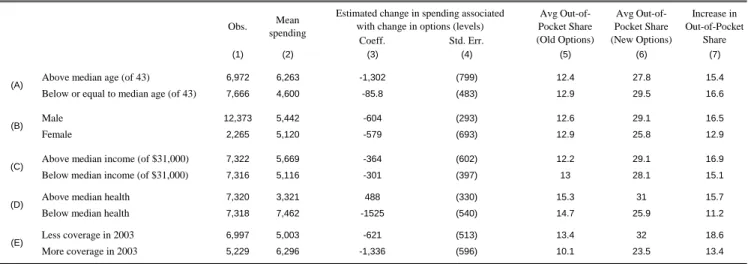
Table 7 presents additional suggestive evidence of heterogeneous (level or proportional) moral hazard e¤ects by reporting the di¤erence-in-di¤erences estimates separately for observably di¤erent groups of workers. Speci…cally, we show the estimated reduction in spending associated with the change from the old to the new options separately for workers above and below the median age (panel A), male vs. female workers (panel B), workers above and below the median income (panel C), and workers of above and below median health risk score (panel D). We discuss the …nal panel (panel E) later.
A di¢ culty with trying to infer heterogeneity in moral hazard from heterogeneous changes in spending across demographic groups is that di¤erential changes in spending may re‡ect either heterogeneous treatment e¤ects (the object of interest) or heterogeneous treatments (i.e., greater changes in cost sharing for some groups than for others, given their endogenous plan choices). Separating these two requires a more explicit model of plan choices as well as how the cost sharing features of the plan a¤ect the spending decision. Again, we do this formally in the context of the model we develop below. However, to get a loose sense of the variation in the change in cost sharing across groups, in columns (5) and (6) we report the average out of pocket share for each demographic group under the old and new options; column (7) reports the increase in the average out of pocket share associated with the change in options, which provides a metric by which to measure the treatment.
The estimates in Table 7 – while generally not precise – are suggestive of heterogenous moral hazard. The top two rows show that the reduction in spending associated with the new options is an order of magnitude higher for older workers than for younger workers, despite what appears to be a somewhat larger increase in the average out of pocket share for the younger workers (column (7)). Panel B indicates similar point estimates for male and female workers, despite the fact that males experience a larger increase in the out of pocket share. Similarly, panel C indicates similar point estimates for higher and lower income workers, but a somewhat larger increase in the out of pocket share for higher income workers. Finally, panel D indicates that the less healthy experience a substantial decline in spending while the more healthy experience no statistically detectable decline in spending, despite a larger increase in the out of pocket share for the more healthy.
While many of the estimates are quite imprecise, the results are suggestive of larger behavioral responses to consumer cost sharing for older workers than younger workers and for sicker workers than healthier workers, and perhaps also for female workers relative to male workers and for lower income workers relative to higher income workers. While suggestive, this type of exercise also points to the limitations of inferring heterogeneity in moral hazard across individuals from such simple descriptive evidence. For example, the parameterization of the “treatment” e¤ects by the average
2 1
Kowalski (2010) …nds similar patterns in her quantile treatment estimates using a di¤erent identi…cation strategy in a di¤erent …rm.
out of pocket share obscures both the endogenous plan choice from within the menu of options as well as the di¤erent expected (end of year) marginal price faced by di¤erent individuals in the same plan based on their health status, which in principle should guide their utilization decisions.
Selection on moral hazard As discussed in the introduction, the pure comparative static of
selection on moral hazard (holding all other factors that determine plan choice constant) is that individuals with a greater behavioral response to coverage (i.e., a larger moral hazard e¤ect) will choose greater coverage. We therefore look for descriptive evidence of the relationship between an individual’s behavioral responsiveness to coverage and their coverage choice. Some suggestive evidence of selection on moral hazard comes from the fact that older workers and sicker workers – whom we saw in Panel A may have larger moral hazard e¤ects than younger workers and healthier workers respectively –also choose more comprehensive insurance under both the new and original plan options (not shown). Of course, older and sicker workers also have higher medical spending so that it is di¢ cult to know from this evidence alone whether their insurance choice is driven by their expected health or their anticipated behavioral response to coverage.
Slightly more direct evidence of selection on moral hazard comes from comparing the estimated behavioral response (estimated by examining the change in spending with the change from the original to the new options) between those who chose more vs. less coverage under the original options. The last panel of Table 7 presents the estimated treatment e¤ect of the move from the original to the new options separately for individuals who chose more coverage under the original options in 2003 compared to those who chose less coverage under the original options in 2003.22 Consistent with selection on moral hazard, we estimate a reduction in spending associated with the move from the old options to the new options that is more than twice as large for those who originally had more coverage than those who originally had less coverage, even though the reduction in cost sharing associated with the change in options (i.e., the treatment) is substantially larger for those who had less coverage. We do not have enough precision, however, to reject the null that estimated spending reductions are the same across the two groups. Moreover, we are once again confronted with the need to model the endogenous plan choice from among the new option as well as the variation in expected end of year marginal price induced by variation in health status.
Overall, we view the …ndings as suggestive descriptive evidence of selection on moral hazard of the expected sign. The rest of the paper now investigates this phenomenon more formally by developing and estimating a model of individual coverage choice and health care utilization. The model allows us to formalize more precisely the notion of “moral hazard,” and aids in the identi…cation of heterogeneity in moral hazard and selection on it. It also allows us to quantify selection on moral hazard and explore its implications through various counterfactual exercises.
2 2Speci…cally, we compare individuals who picked option 3 (“more coverage”) under the original options to those who picked option 2 (“less coverage”) under the original options. To do this analysis we need to limit the sample to the approximately 85 percent of the sample who was already employed at the …rm by 2003 and in one of these two options. The estimated change in spending associated with the move from the old to the new options for this subsample is -859 (standard error 245), compared to -592 (standard error 264) in the full 2003-2006 sample (Table 5, column (4)).
4
A model of coverage choice and utilization
We now present a stylized model of individual coverage choice and health care utilization which we will then use as the main ingredient in our econometric speci…cation and counterfactual exer-cises. The model is designed to allow us to isolate and examine separately three di¤erent potential determinants of insurance coverage choice: health expectations, risk aversion, and “moral hazard type.”
We consider a two period model. In the …rst period, a risk-averse expected-utility maximizing individual makes an optimal health insurance coverage choice, using his available information to form his expectation regarding his subsequent health realization. In the second period, the in-dividual observes his realized health and makes an optimal health care utilization decision, which depends on the realized health as well as on his coverage. It is this last e¤ect which leads to what we call moral hazard. This general modeling framework is similar to the one used in existing empirical models of demand for health insurance and medical spending (Cardon and Hendel, 2001; Bajari et al., 2010; Carlin and Town, 2010; Handel, 2010).
We begin with notation. This is a model of individual behavior, so we omit i subscripts to simplify notation; in the next section, where we take the model to the data, we describe how individuals may vary. At the time of his utilization choice (period 2), an individual is characterized by two objects: his health realization , and his “moral hazard type”!. The health realization captures the uncertain aspect of demand for healthcare, with individuals with higher being sicker and demanding greater healthcare consumption. The moral hazard type ! determines how responsive health care utilization decisions are to insurance coverage. In other words, !a¤ects the individual’s price elasticity of demand for healthcare with respect to its (out of pocket) price, with individuals with higher ! being more price elastic and therefore increasing their utilization more sharply in response to greater insurance coverage.
At the time of coverage choice (period 1), an individual is characterized by three objects:F ( ),
!, and . The …rst, F ( ), represents the individual’s expectation about his subsequent health risk . It is precisely the (natural) assumption that individuals do not know with certainty at the time of coverage choice, which leads them to demand insurance. The second object that enters the individual’s coverage choice is his moral hazard type !, which determines his period 2 price elasticity of demand for health care. Because individuals are forward looking, they anticipate that their price sensitivity will subsequently a¤ect their utilization choices, and this in turn a¤ects their utility from di¤erent coverages. It is this channel that creates the potential for selection on moral hazard, which is the main focus of our paper. Finally, the third object is , which captures the individual’s coe¢ cient of absolute risk aversion. Importantly, unlike ! and F ( ), which enter the coverage choice but also a¤ect (deterministically and stochastically, respectively) utilization decisions, risk preferences a¤ect coverage choice but play no direct role in utilization decisions.
Utilization choice In the second period, insurance coverage, denoted by j, is taken as given.
tradeo¤ between health and money, with higher ! individuals putting greater weight on health. Speci…cally, we assume that the individual’s second period utility is separable in health and money and can be written as u(m; ; !) =h(m ;!) +y(m), where m 0 is the monetized utilization choice, is the monetized health realization, and y(m) is the residual income. Naturally, y(m) is decreasing in m at a rate that depends on coverage. In contrast, we assume that h(m ;!) is concave in its …rst argument, so that it is increasing for low levels of utilization (when treatment presumably improves health) and is decreasing eventually (when there is no further health ben-e…t from treatment and time costs dominate). Thus, we assume that the marginal benben-e…t from incremental utilization is decreasing. Using this formulation, we think of , the underlying health realization, as shifting the level of optimal utilization m . Finally, we assume that h(m ;!) is increasing in its second argument, but this is purely a normalization which (as we will see below) allows us to interpret individuals with higher ! as those who are more elastic with respect to the price of medical utilization.
We parametrize further so that the second-period utility function is given by
u(m; ; !; j) = (m ) 1 2!(m ) 2 | {z } + [y cj(m) pj] | {z } h(m ;!) y(m) : (1)
That is, we assume that h(m ;!) is quadratic in its …rst argument, with! a¤ecting its curva-ture. We also explicitly write the residual income as the initial income y minus the premium pj
associated with coverage j and the out-of-pocket expenditurecj(m) associated with utilizationm
under coveragej. Becausey and pj are taken as given (at the time of utilization choice), it will be
convenient to de…ne e u(m; ; !; j) = (m ) 1 2!(m ) 2 c j(m); (2) so that u(m; ; !; j) =eu(m; ; !; j) +y pj.
Given this parameterization, the optimal utilization is given by
m ( ; !; j) = arg max
m 0u(m; ; !; j): (3)
It will also be convenient to denoteu ( ; !; j) u(m ( ; !; j); ; !; j)andue ( ; !; j) ue(m ( ; !; j); ; !; j). To facilitate intuition, we consider here optimal utilization for the case of a linear (i.e., constant
coinsurance) coverage contract, so that cj(m) =c m where c 2[0;1]. Full insurance is therefore
given by c = 0 and no insurance is given by c = 1. The …rst order condition implied by the optimization problem in equation (3) is therefore given by1 !1(m ) c= 0, or
m ( ; !; c) = max [0; +!(1 c)]: (4)
Thus, abstracting from the potential truncation of utilization at zero, the individual will spend
m = with no insurance (i.e., c= 1) and m = +! with full insurance (i.e.,c= 0). Thus, the utilization response to the change in coverage from full to no insurance is !; utilization responds
more to changes in coverage for individuals of greater moral hazard type (i.e., higher!). One way to think about this model of moral hazard, therefore, is that represents non-discretionary health care shocks that all individuals will pay to treat, regardless of insurance. There is also discretionary health care utilization (such as whether to go to the doctor when confronted with a minor pain or irritation, for example) which, without insurance will not be undertaken. With insurance, some amount of this discretionary care will be consumed, with individuals with a higher ! consuming more of this discretionary care when they are insured.23
Coverage choice In the …rst period, the individual faces a fairly standard insurance coverage
choice. As mentioned, we assume that the individual is an expected-utility maximizer, with a coe¢ cient of absolute risk aversion of . We further assume that the individual’s von Neumann Morgenstern (vNM) utility function is of the constant absolute risk aversion (CARA) form,w(x) = exp( x). In a typical insurance settingw(x)is de…ned solely over …nancial outcomes. However, because moral hazard is present, individuals trade o¤ income and health and therefore w(x) is de…ned over the realized second-period utility u ( ; !; j). We note that income enters u ( ; !; j)
additively with a coe¢ cient of one, sou ( ; !; j)is monetized and can still be thought of in dollars, as in the regular case.
Consider now a set of coverage options J, with each option j 2 J de…ned by its premium pj
and coverage function cj(m). Following the above assumptions, the individual will then evaluate
his expected utility from each option,
vj(F ( ); !; ) =
Z
exp( u ( ; !; j))dF ( ); (5)
with his optimal coverage choice given by
j (F ( ); !; ) = arg max
j2J vj(F ( ); !; ): (6)
Measuring welfare and e¢ cient contracts Our standard measure of consumer welfare in this
context will be the notion of certainty equivalent. That is, for an individual de…ned by(F ( ); !; ), we denote the certainty equivalent to a contract j by the scalar ej that solves exp( ej) =
vj(F ( ); !; ), or ej(F ( ); !; ) 1 ln Z exp( u ( ; !; j))dF ( ) : (7)
Our assumption of CARA utility over (additively separable) income and health implies no income e¤ects. To see the implications of no income e¤ects, we can substituteu ( ; !; j) =eu ( ; !; j)+y pj
2 3
We have written the model as if it is the individual who makes all the utilization decisions. In practice, many of the decisions are also a¤ected by physicians. To the extent that physicians also respond to the individual’s coverage (and they are likely to), our interpretation of moral hazard should be thought of as some combination of both the individual’s and the physician’s responses.
into equation (7) and reorganize to obtain ej(F ( ); !; ) eej(F ( ); !; ) +y pj (8) 1 ln Z exp( ue ( ; !; j))dF ( ) +y pj;
so that eej(F ( ); !; ) captures the welfare from coverage, and residual income enters additively.
Using this notation, di¤erences in ee( ) across contracts with di¤erent coverages capture the will-ingness to pay for coverage. For example, an individual de…ned by(F ( ); !; ) is willing to pay at mosteek(F ( ); !; ) eej(F ( ); !; ) in order to increase his coverage fromj tok.
Equation (8) can also be used to characterize the comparative statics of willingness to pay for more coverage with respect to the model’s primitives. In general, willingness to pay for more coverage is increasing in risk aversion and in risk F ( ) (in a …rst order stochastic dominance sense).24 Given our speci…c parametrization, willingness to pay for more coverage is also increasing in moral hazard type !.25
We assume that insurance providers are risk neutral, so that the provider’s welfare is given by his expected pro…ts, or
j(F ( ); !) pj
Z
[m ( ; !; j) cj(m ( ; !; j))]dF ( ); (9)
where the integrand captures the share of the utilization covered by the provider under contractj. Total surplus sj is then given by
sj(F ( ); !; ) =ej(F ( ); !; )+ j(F ( ); !) =eej(F ( ); !; )+y
Z
[m ( ; !; j) cj(m ( ; !; j))]dF ( ):
(10) That is, total surplus is simply certainty equivalent minus expected cost.
Finally, it may be useful to characterize the nature of the e¢ cient contract in this setting. Because of our CARA assumptions, premiums are a transfer which do not a¤ect total surplus. Therefore, the e¢ cient contract can be characterized by the e¢ cient coverage function c ( ) that maximizes total surplus (as given by equation (10)) over the set of possible coverage functions. Such optimal contracts would trade o¤ two o¤setting forces. On one hand, an individual is risk averse while the provider is risk natural, so optimal risk sharing implies full coverage, under which the individual is not exposed to risk. On the other hand, the presence of moral hazard makes an insured individual’s privately optimal utilization choice socially ine¢ cient; any positive insurance coverage
2 4
These comparative statics do not always hold. The model has unappealing properties when a signi…cant portion of the distribution of is over the negative range, in which case the individual is exposed to a somewhat arti…cial uninsurable (background) risk (since spending is truncated at zero). We are not particularly concerned about this feature, however, as our estimated parameters do not give rise to it, and because we have experimented with a (non-elegant) modi…cation to the model that does not have this feature, and the overall results were similar.
2 5
In a more general model, ! is associated with two e¤ects. One is the increased utilization, which increases willingness to pay. The second e¤ect is the increased ‡exibility to adjust utilization as a function of the realized uncertainty ( ), which in turn reduces risk exposure and reduces willingness to pay for insurance. Our speci…c parameterization was designed to have spending under no insurance una¤ected by!; this eliminates this latter e¤ect, and therefore makes the comparative statics unambiguous.
makes the individual face a healthcare price which is lower than the social cost of healthcare, leading to excessive utilization. E¢ cient contracts will therefore resolve this tradeo¤ by some form of partial coverage (Arrow, 1971; Holmstrom, 1979). For example, it is easy to see that no insurance (c (m) =m) is e¢ cient if individuals are risk neutral or face no risk (F ( )is degenerate), and that full insurance (c (m) = 0) is e¢ cient when moral hazard is not present (! = 0). In all other· situations, the e¢ cient contract is some form of partial insurance.
Discussion Before turning to estimation, a few of our speci…c modeling choices above merit some
further discussion.
Terminology. The key conceptual distinction we are interested in is the possibility that selection is not only driven by “traditional”selection, on the expected level of medical expenditures (F ( )), but also by selection on the basis of the incremental medical expenditure with respect to increased coverage (!). We refer to this latter e¤ect as “moral hazard.”
The use of the term “moral hazard” to refer to the responsiveness of medical care utilization to insurance coverage dates back at least to Arrow (1963). Consistent with the notion of “hidden action” – as is typically associated with the term “moral hazard" – it has been conjectured that health insurance may induce individuals to exert less (unobserved) e¤ort in maintaining their health. However, in the context of health insurance the term “moral hazard”is more typically used to refer to the price elasticity of demand for health care, conditional on underlying health status (Pauly, 1968; Cutler and Zeckhauser, 2000). We thus follow this abuse of terminology, and use the term in a similar way. In other words, our model, like most in this literature, does not consider the potential impact of insurance on underlying health .
As a result, the asymmetric information problem that we associate with “moral hazard” is arguably more accurately described as one of hidden information (rather than of hidden action). The individual’s actions (utilization) are observed and contractible, but his underlying health is hidden information which, if contractible, would be the e¢ cient object of reimbursement. For our purposes, whether the problem is one of hidden information or hidden action is simply an issue of appropriate usage of terminology, and here we simply follow convention.26
Additive e¤ ect of moral hazard. We made the strong choice to model moral hazard (!) as a level shift in spending that is (except due to the truncation of spending at zero) independent of one’s health ( ) (see, e.g., equation (4)). This is primarily for analytical tractability. Our choice of the utility function in equation (1) is designed to achieve a straightforward economic interpretation of the key parameters of interest in the …rst order condition (4). In particular, it is designed so that (health status) is the monetized health spending without insurance (i.e., one’s “nondiscretionary” spending), and ! (moral hazard) captures incremental, “discretionary” spending as individuals
2 6There are two potential justi…cations given in the literature for why the impact of insurance on medical expendi-tures, conditional on health status, may constitute hidden action. First, patients and physicians may take less e¤ort to shop around for better prices when they are insured (Arrow, 1963). Second, if insurance a¤ects the quantity of care consumed, Cutler and Zeckhauser (2000) argue that this still constitutes hidden action since “though the action itself (seeking medical care) is not hidden, the motivation behind it is.”