Curtis Carlson, Dallas Burtraw,
Maureen Cropper, and Karen Palmer
Discussion Paper 98-44-REV
April 2000
RESOURCES
for the future
1616 P Street, NW Washington, DC 20036 Telephone 202-328-5000 Fax 202-939-3460
Internet: http://www.rff.org
©2000 Resources for the Future. All Rights Reserved. No portion of this paper may be reproduced without permission of the authors.
Discussion papers are research materials circulated by their authors for purposes of information and discussion. They have not undergone formal peer review or the editorial treatment accorded RFF books and other publications.
Abstract
Title IV of the 1990 Clean Air Act Amendments (CAAA) established a market for transferable sulfur dioxide (SO2) emission allowances among electric utilities. This market offers firms facing high marginal abatement costs the opportunity to purchase the right to emit SO2 from firms with lower costs, and is expected to yield cost savings compared to a command and control approach to environmental regulation. This paper uses econometrically estimated marginal abatement cost functions for power plants affected by Title IV of the CAAA to evaluate the performance of the SO2 allowance market. Specifically, we investigate whether the much-heralded fall in the cost of abating SO2, compared to original estimates, can be attributed to allowance trading. We demonstrate that, for plants using low-sulfur coal to reduce SO2
emissions, technical changes and the fall in low-sulfur coal prices have lowered marginal
abatement cost curves by over 50% since 1985. The flexibility to take advantage of these changes is the main source of cost reductions, rather than trading per se. In the long run, allowance trading may achieve cost savings of $700-$800 million per year compared to an “enlightened” command and control program characterized by a uniform emission rate standard. The cost savings would be twice as great if the alternative to trading were forced scrubbing. However, a comparison of potential cost savings in 1995 and 1996 with actual emissions costs suggests that most trading gains were unrealized in the first two years of the program.
Key Words: acid rain, sulfur dioxide, air pollution, Clean Air Act, Title IV, permit trading JEL Classification Nos.: H43, Q2, Q4
III. Methodology...6
A. Calculation of the Gains from Allowance Trading...6
The Role of Scrubbing vs. Fuel-switching...7
Computation of the Gains from Trade...8
B. Estimation of Marginal Abatement Cost Curves ...8
Econometric Model...9
Data...12
Results of the Estimation...13
Table 1: 1985 and 1994 Weighted Average Marginal Abatement Costs and SO2 Emission Rates for Coal-Fired Units without Scrubbers...14
Figure 1: Low-Sulfur and High-Sulfur Coal Prices...15
Figure 2: The Effect of Changes in Fuel Prices and Technical Change on Marginal Abatement Cost Functions...16
IV. The Least-Cost Solution and Potential Gains from Trade in the Long Run ...17
A. Preferred Estimates of the Least-Cost Solution...17
Electricity Output...17
Input Prices and Technical Change ...17
Retirement of Coal-Fired Power Plants ...18
Baseline Emissions...18
Continuous Emissions Monitoring Data...18
Minimum Compliance Costs in the Preferred Case...18
B. Comparisons and Sensitivity Analyses...19
Table 2: Long-Run (Phase II, year 2010) Cost Estimates...20
C. Potential Gains from Trade ...21
V. The Performance of the Allowance Market in 1995 and 1996...23
Table 3: Phase I (1995 and 1996) Cost Estimates ...23
VI. Conclusions...25
Appendix A...27
Appendix B...30
Emission Equation and Cost Function Parameter Estimates ...30
SO2 CONTROL BY ELECTRIC UTILITIES:
WHAT ARE THE GAINS FROM TRADE?*
I. INTRODUCTION
For years economists have urged policy makers to use market-based approaches to control pollution (taxes or tradable permits) rather than relying on uniform emission standards or uniform technology mandates (command and control). This advice was largely ignored until the 1990 Clean Air Act Amendments (CAAA) established a market for sulfur dioxide (SO2) allowances. Coupled with a cap on overall annual emissions, the SO2 allowance market gives electric utilities the opportunity to trade rights to emit SO2 rather than forcing them to install SO2 abatement technology or emit at a uniform rate. By equalizing marginal abatement costs among power plants, trading should limit SO2 emissions at a lower cost than the traditional command and control approach.
The SO2 allowance market presents the first real test of the wisdom of economists' advice, and therefore merits careful evaluation. Has the allowance market significantly lowered the costs of abating SO2, as economists claimed it would? An answer in the affirmative would strengthen the case for marketable permits to control other pollutants, such as greenhouse gases. Conversely, if cost savings are small, this would have implications for the design (or even the adoption) of market-based approaches to controlling pollution in the future.
The purpose of this paper is to evaluate the performance of the SO2 allowance market. Specifically, we ask two questions: (1) How much can the trading of permits reduce the costs of controlling SO2, compared to command and control; i.e., what are the potential gains from trade? (2) Were these trading gains realized in the first years of the allowance market? The answers require that we estimate marginal abatement cost functions for fuel switching at all generating units that do not scrub their emissions, calculate the expected cost of post-combustion abatement (scrubbers), and compute the least-cost solution to achieving the cap on SO2 emissions. The difference between the least-cost solution and the cost under our counter-factual command and control policy represents the potential static efficiency gains from allowance trading. We compute these gains for 1995 and 1996, the first two years of the allowance market, and the expected savings in 2010, when the emissions cap will be stricter and applied more broadly and when the allowance market should be functioning as a mature market.
* * This paper has benefited from comments and suggestions from Robert Chambers, Denny Ellerman, Suzi Kerr, Richard Newell, Paul Portney and Byron Swift. We would especially like to thank Don Fullerton for his
exceptionally detailed comments which have significantly improved the paper. Carlson's work on this paper was not part of his official duties at the National Oceanic and Atmospheric Administration (NOAA) and his employment with NOAA does not constitute an endorsement by the agency of the views expressed in this paper. This paper does not represent the views of the World Bank, its Executive Directors, or the countries they represent. The authors are grateful to the Environmental Protection Agency for partial support of this study.
The command and control policy against which we measure gains from allowance trading is key to the analysis. A policy that would have imposed end-of-stack abatement technology (scrubbing) would have been significantly more expensive than an emission rate standard applied uniformly to all facilities.1 A uniform emission rate standard provides firms with considerable flexibility, including the opportunity to take advantage of technical change that is precluded under a more rigid technology standard; hence it is a favorable characterization of a command and
control approach. In our analysis we evaluate the gains from allowance trading compared to each of two command and control alternatives–forced scrubbing and a uniform emission rate
standard.2
Our approach to evaluating the allowance market is very different from the approach used by other observers to assess market performance. Both the Administrator of the USEPA and the chair of the Council of Economic Advisors proclaimed the success of the allowance market by comparing allowance prices (circa $100 per ton in 1997) with estimates of marginal abatement costs produced at the time the CAAA were written (as high as $1500).3 Since the former are
much lower than the latter, they concluded that the trading of SO2 allowances has greatly reduced the cost of curbing SO2 emissions.
This argument is flawed for two reasons. First, it is inappropriate to judge how well the allowance market is performing simply by comparing current allowance prices with ex ante estimates of marginal abatement costs in the least-cost solution. Price can equal marginal abatement cost even if many utilities that might benefit from trading fail to participate in the market. Second, comparing current allowance prices with ex ante estimates of marginal abatement costs shows only that the latter were too high; it does not mean that the allowance market was responsible for the fall in marginal abatement costs.4
Our analysis suggests that the above claims for the allowance market are misleading— especially the suggestion that formal trading has lowered the cost of SO2 abatement several fold. In contrast, we reach the following conclusions:
(1) Marginal abatement costs for SO2 are much lower today than were estimated in 1990. Technical improvements including advances in the ability to burn low-sulfur coal at existing generators, as well as improvements in overall generating efficiency, lowered the typical unit's
1. In 1983 the Sikorski/Waxman bill sought to reduce SO2 emissions by requiring the installation of scrubbers (flue
gas desulfurization equipment) at the fifty dirtiest plants. Studies estimate that the annual cost of this proposal would have ranged from $7.9 billion (OTA, 1983) to $11.5 billion (TBS, 1983), in 1995 dollars.
2. One justification for the use of an emission rate standard is that it is the approach used to regulate NOx emissions under Title IV of the 1990 Clean Air Act Amendments.
3. On March 10, 1997 EPA Administrator Carol Browner argued: “...During the 1990 debate on the acid rain program, industry initially projected the cost of an emission allowance to be $1500 per ton of sulfur
dioxide...Today, those allowances are selling for less than $100." ("New Initiatives in Environmental Protection,"
The Commonwealth, March 31, 1997.) Likewise, in testimony before Congress, CEA Chair Janet Yellen noted, "Emission permit prices, currently at approximately $100 per ton of SO2 are well below earlier estimates . . ..
Trading programs may not always bring cost savings as large as those achieved by the SO2 program . . . "
(Yellen 1998).
4. It should also be noted that the ex ante estimates of marginal abatement costs were generally for the second phase of the program, and therefore cannot be compared with current allowance prices unless they are discounted to the present.
marginal abatement cost function by almost $50 dollars per ton of SO2 over the decade preceding 1995. The decline in fuel costs lowered marginal abatement costs by about $200 per ton.
(2) This decline in marginal abatement cost, assuming that it was not caused by Title IV, has lowered the cost of achieving the SO2 emission cap under both the least-cost solution and under enlightened command and control (e.g., under a uniform emission rate standard). This implies that the gains from trade—the cost savings attainable from an allowance trading program—have also fallen over time.5 We estimate the potential cost savings attributable to formal trading (vs. a uniform emission rate standard) to be $250 million (1995 dollars) annually during the first phase of the allowance program (1995–2000, which covers the dirtiest power plants). We estimate them to be $784 million annually during the second phase of the program (beginning in 2000, which covers all plants), about 43% of compliance costs under our
enlightened command and control policy. A comparison of the least-cost solution with a less enlightened command and control alternative of forced scrubbing indicates annual savings of almost $1.6 billion (1995 dollars).
(3) Comparing the least-cost solution to achieving actual emission reductions with actual abatement costs indicates that actual compliance costs exceeded the least-cost solution by $280 million in 1995, and by $339 million in 1996 (1995 dollars). This suggests that the allowance market did not achieve the least-cost solution, even though marginal abatement costs under that solution were approximately equal to allowance prices. The failure to realize potential savings is not surprising. The 1990 Clean Air Act Amendments represent a dramatic departure from the pollution regulations to which utilities were previously subject; and taking full advantage of their flexibility may require time. As participants become more familiar with the opportunities
presented by the allowance market, and ongoing deregulation of the electricity industry provides greater incentives to reduce costs, the volume of trading will no doubt increase and cost savings are more likely to be realized.
The remainder of the paper is organized as follows. Section II provides institutional background on the CAAA. Section III presents the methodology we employ to evaluate the allowance market, including our estimation of marginal abatement cost curves. Section IV
estimates potential gains from allowance trading in the long run, and explains why these estimates are lower than were predicted when the CAAA were written. Section V evaluates the
performance of the allowance market in 1995 and 1996, and section VI concludes the paper.
II. INSTITUTIONS
Since 1970, the SO2 emissions of electric utilities have been regulated in order to achieve federally mandated local air quality standards (the National Ambient Air Quality Standards). For plants in existence in 1970 these standards, codified in State Implementation Plans, have
5. The assumption that the fall in marginal abatement costs was not due to Title IV potentially imparts a downward bias to the estimate of the cost savings under the program. The incentives provided by allowance trading might have accelerated changes in fuel prices, as well as other technological changes (Burtraw 1996).
typically taken the form of maximum emission rates (pounds of SO2 per million Btus of heat input). Plants built after 1970 are subject to New Source Performance Standards (NSPS), set at the federal level. Since 1978, NSPS for coal-fired power plants have effectively required the installation of capital-intensive flue gas desulfurization equipment (scrubbers) to reduce SO2 emissions, an attempt to protect the jobs of coal miners in states with high-sulfur coal. This regulation has significantly raised the costs of SO2 abatement at new plants in areas where emissions could have been reduced more cheaply by switching to low-sulfur coal.
During the 1980s, over 70 bills were introduced in Congress to reduce SO2 emissions from power plants. Some would have forced the scrubbing of emissions by all electric generating units, while others would have provided limited flexibility by imposing uniform emission rate standards, which give firms the opportunity to chose a compliance strategy.
The innovation of Title IV is to move away from these types of uniformly applied regulations. Instead, reductions are to be achieved by setting a cap on emissions while allowing the trading of marketable pollution permits or allowances. Each generating unit in the electricity industry is allocated a fixed number of allowances each year, and is required to hold one
allowance for each ton of sulfur dioxide it emits.6 Utilities are allowed to transfer allowances among their own facilities, sell them to other firms, or bank them for use in future years.
The eventual goal of Title IV of the CAAA is to cap average annual SO2 emissions of electric utilities at 8.95 million tons—about half of their 1980 level. This is to be achieved in two phases. In the first phase, which began in 1995, each of the 110 dirtiest power plants (with 263 generating units) are allocated allowances sufficient for an emission rate of 2.5 pounds SO2 per mmBtu of heat input. Firms can voluntarily enroll additional generating units (“Compensation and Substitution” units) in Phase I, subject to the constraint that the average emission rate of all units does not increase. In the second phase, which begins in the year 2000, all fossil-fueled power plants larger than 25 megawatts are annually allocated allowances sufficient for an
emission rate of 1.2 pounds of SO2 per mmBtu heat input. In both phases, heat input is based on the 1985–1987 reference period.
Allowance trading takes advantage of the fact that emission control costs vary across generating units, and encourages firms with the cheapest control costs to undertake the greatest emission reductions. Unfortunately, firms may not have adequate incentives to minimize SO2 compliance costs because of decisions made by some state public utility commissions (Rose
6. Allowances are allocated to units in proportion to emissions during the 1985–1987 period. About 2.8% of the annual allowance allocations are withheld by the EPA and distributed to buyers through an annual auction run by the Chicago Board of Trade. The revenues are returned to the utilities that were the original owners of the allowances. An emissions cap creates a barrier to entry and commensurate scarcity rents that accrue to owners of existing facilities when allowances are allocated at zero cost to these facilities. These rents would not be present in our command and control (performance standard) policy. Fullerton and Metcalf (1997) show that these rents compound economic distortions associated with preexisting taxes, thereby imposing an important source of additional social cost not reflected in firms’ compliance costs. Goulder, Parry and Burtraw (1997) find this additional social cost to be of similar magnitude to the compliance cost savings from allowance trading that we identify. Theyfind the social cost of an emissions cap could be largely alleviated were the program to auction allowances and use the revenue to reduce preexisting labor taxes.
(1997); Bohi (1994); Bohi and Burtraw (1992). For instance, to protect the jobs of miners in high-sulfur coal states, some regulators pre-approved the recovery of investment in scrubbers, while leaving uncertain whether or not the cost of other possible compliance measures would be similarly recoverable. The allowance program itself encouraged scrubbing by allocating 3.5 million “bonus” allowances to firms that installed scrubbers as the means of compliance, for the explicit purpose of protecting jobs in regions with high-sulfur coal. In addition, investments in scrubbers can be depreciated and in some cases expensed (deducted against income tax) as soon as the scrubber is installed. In contrast, in many states the cost of purchased allowances cannot be recovered until they are used for compliance.7 These facts suggest that — through no fault of its own — the allowance market might not succeed in capturing the potential gains from emission trading, a hypothesis that we investigate below.8
III. METHODOLOGY
To investigate whether the allowance market has operated efficiently and to estimate the size of potential gains from trading versus other forms of regulation, we estimate marginal abatement cost functions for generating units. These functions can be used to calculate the least-cost solution to achieving an aggregate level of emissions, as well as the expected least-costs of
alternative regulatory approaches.
A. Calculation of the Gains from Allowance Trading
The least-cost solution to achieving the SO2 cap requires minimizing the present
discounted value of compliance costs for all generating units over time, subject to constraints on the banking of allowances. Because the SO2 cap shrinks between Phase I and Phase II, the
banking of allowances will, in general, be optimal (if adjustment costs for reducing pollution are not too great). Thus emissions should be less than allowances in the early years of the program (Rubin, 1996). Eventually, however, a steady state is expected in which net contributions to the bank are zero on average, and annual emissions equal annual allowances. Rather than solve this inter-temporal problem, we sidestep the banking question by taking the banking behavior of firms as given.9
Our primary goal is to compute how much more cheaply the chosen level of emissions could be achieved through formal trading within the allowance market than by a uniform emission standard. We calculate the long run gains from trade by computing the least-cost solution to achieving the emissions cap in the year 2010, when annual allowances should equal annual
emissions (EPA, 1995; EPRI, 1997). We then contrast this solution with the cost of achieving the cap in 2010 via a uniform emission rate standard (an “enlightened” form of command and control)
7. Lile and Burtraw (1998).
8. Fullerton, McDermott and Caulkins (1997) and Winebrake et al. (1995) provide estimates of the potential magnitude of inefficiencies that may result, but no author has attempted to estimate actual performance.
and with the cost of achieving the cap via forced scrubbing. For 1995 and 1996, the first two years of the allowance market, we compute the potential gains from trade as the difference between the least-cost solution to achieving actual emissions and the cost of achieving these emissions via enlightened command and control. We then calculate the costs actually incurred in these two years, to learn whether the potential gains from trading have been realized.
The Role of Scrubbing vs. Fuel-switching
To calculate the least-cost solution to limiting SO2 emissions, we must estimate the
marginal abatement cost curves of all generating units in the allowance market. In estimating marginal abatement cost functions, we separate plants into those that reduce SO2 emissions via fuel-switching (substituting low-sulfur for high-sulfur coal) and those that have installed
scrubbers. As noted above, fuel switching is the chief method of reducing emissions for most power plants. In 1995 only 17 percent of all generating units in the United States used scrubbers. Eighty-six percent of these units were required to do so by law, either to satisfy federal New Source Performance Standards (61%) or state laws (24%). The remaining 15% of units (28 in number) installed scrubbers specifically to comply with Title IV. We assume that units which were required by law to scrub or which chose to do so in Phase I continue to do so in the least-cost solution as well as in the command-and-control counterfactual. Hence, the least-cost of scrubbing at these units is added to the total abatement costs under both scenarios and does not directly affect our estimates of the cost savings from efficient trading.
To see whether additional firms would build scrubbers to minimize compliance costs, we solve for the marginal cost of abatement under fuel switching and compare this with the average cost of abatement via scrubbing. If the marginal cost of abatement under fuel switching is lower than the average cost of abatement under scrubbing, as we find it to be, building additional retrofit scrubbers would not lower costs.10
From the perspective of abating SO2 emissions, the chief difference between units that
fuel switch and units that scrub is the shape of their marginal abatement cost (MAC) functions. Holding electricity output constant, plants that fuel switch can reduce the tons of SO2 they emit
by varying the sulfur content of their fuel. Assuming that a premium must be paid per million Btu for low-sulfur coal, this implies that the marginal abatement cost curve slopes down as emissions of SO2 increase.11 For plants that scrub, emissions of SO2 are almost entirely
determined by electricity output (heat input). Because scrubbers remove about 95% of the sulfur content of coal, emissions are relatively insensitive to the sulfur content of coal burned.
Conditional on output, therefore, the marginal abatement cost curve for scrubbed units is a point. In computing the least-cost solution and the command and control alternative, we therefore
10. A referee suggests that this comparison should be made using a plant-specific average cost of scrubbing; however, we do not have enough data to calculate an average cost of scrubbing for each coal-fired generating unit in our dataset. We compare marginal abatement cost (permit price) in the least-cost solution with average abatement cost under scrubbing based on the 28 units that installed retrofit scrubbers.
11. The marginal abatement cost curve slopes downward because in our long run cost function capital is fully adjustable and increased capital investments are required to increase the amount of low-sulfur coal burned, in addition to paying a per mmBtu premium for low- (vs. high-) sulfur coal.
subtract the emissions of scrubbed units from the emissions cap and solve for the least-cost solution using the estimated marginal abatement cost curves of units that fuel switch.
Formally, we choose the level of emissions for each fuel-switching unit that minimizes the aggregate cost of achieving the modified overall emissions cap. In general, a generating unit’s marginal cost of emissions function depends on output (as well as on emissions and input prices); however, we do not vary electricity output to reduce SO2. We thus ignore demand-side management as an emissions reduction strategy, as well as the possibility of shifting output from dirty to clean plants to reduce SO2.12
Computation of the Gains from Trade
From a baseline of emissions that would have obtained absent the 1990 Clean Air Act Amendments, we compute the cost of the least-cost solution for all units that fuel switch as the area under their marginal abatement cost (MAC) curves from baseline emissions to emissions under the least-cost solution. For firms whose MAC curves are positive over all relevant
emissions levels, the computation is straightforward. For firms whose marginal abatement curves are negative over some range of emissions, we compute the cost of moving from baseline
emissions to emissions in the least-cost solution as the area under the portion of the MAC curve that lies above the positive quadrant.13 To compute total costs under the least-cost solution and in the command-and-control alternatives, the capital and variable costs of retrofit scrubbing are annualized over twenty years using a 6% discount rate and are added to the costs of fuel switching. The gains from trade are the difference between total costs under the least-cost solution and total costs under the command-and-control counterfactual.
B. Estimation of Marginal Abatement Cost Curves
To estimate marginal abatement cost functions for plants that fuel switch, we assume that the manager of each power plant minimizes the cost of producing electricity at the generating unit, subject to its production technology and a constraint on SO2 emissions. This constraint represents the emissions standard facing the plant because of the National Ambient Air Quality Standards (NAAQS) for SO2.14 We have chosen the generating unit as the unit of analysis
12. In order to switch output among plants, we would have to model the electricity grid, which is beyond the scope of the paper. There is no evidence that utilities have relied on demand-side management to reduce SO2; indeed, the cost per ton of SO2 reduced would be much more expensive if achieved through reductions in output than through fuel switching.
13. Savings at firms with negative abatement costs are not considered cost savings attributable to the trading program. To incorporate units in the least-cost solution for which we have not estimated MAC curves, we allocate allowances, A, to units for which MAC curves are available, solve the least-cost solution, and then multiply total cost by the ratio of total allowances to A. This, in effect, assumes that the aggregate MAC curve for omitted units is identical to that for the units in our dataset.
14. Throughout, we assume that electric utilities comply with local permitting constraints set to meet NAAQS. These are distinct from the requirements of the 1990 Amendments that established the SO2 trading program in order to meet regional air quality goals. The assumption that emissions never violate the emissions standard appears justified by USEPA data, which show that fewer than 5% of the plants in our database were ever in violation of
because SO2 emissions standards apply to individual generating units.15 An alternative approach would be to assume the manager minimizes the cost of producing a fixed level of output at the plant level, equating the marginal cost of electricity generation across generating units, but this would force us to average emission standards across units faced with different standards. Since the order in which units are brought into service is usually pre-determined, we treat output as fixed at the generator level.
Our approach to estimating marginal abatement cost functions at fuel-switching units is to estimate a cost function and share equations for electricity generation that treat generating capital as variable, using data from the period prior to trading under the CAAA. We treat generating capital as variable to capture capital investments that allow plants to burn low-sulfur coal. Because the firm’s desired amount of capital stock is instantaneously achievable in this model, the estimates we obtain are estimates of long-run abatement costs. This is similar to the approach taken by Gollop and Roberts (1983, 1985) who estimated marginal abatement costs at the firm level for 56 coal-fired electric utilities. They examined firms’ responses to SO2 regulations between 1973 and 1979 for firms that met emission requirements through fuel switching.16 Econometric Model
The manager's problem is to choose labor (l), generating capital (k), fuel inputs of high-and low-sulfur coal (fhs high-and fls, respectively) to minimize the cost of producing output (q) high-and achieving an emission rate (e) in time period (t), subject to emissions and production constraints. Unit and time indexes are suppressed for convenience.
* , , , ) , , , , ( ) , , , , ( : subject to Min e t fhs fls l k e Q t fhs fls l k q fhs p fls p l p k p C k l fls fhs fhs fls l k ≤ ≥ + + + = (1) emission regulations during the entire period of our study.
15. Generating units consist of a generator-boiler pair. For over 85% of the generating capacity, there is a one-for-one match between generators and boilers. For the remaining 15%, there are multiple generators attached to a boiler or vice versa. Emission standards and allowance allocations apply to the boiler. The continuous emission
monitoring system used under Title IV measures emissions at the stack level, and it is often the case that several generating units are attached to one emission stack. For those units that share boilers and/or stacks, we assign emissions based on the percentage of total heat input consumed by each boiler. For generators that share a single boiler, we assign emissions based on the percentage of total electricity output from each generator.
16. The econometric estimation of marginal abatement cost functions is distinct from the approach taken in other analyses of Title IV that rely on engineering estimates of marginal abatement cost functions (Fullerton, McDermott and Caulkins (1997), Siegel (1997), Kalagnanam and Bokhari (1995), Burtraw et al. (1998), EPA (1995, 1990), EPRI (1995), and GAO (1994)).
In (1), e* represents the emissions standard, typically stated as an emission rate, e.g., pounds of SO2 per million Btus of heat input, averaged over a specified time interval.17 In deriving the cost function to be estimated, one approach would be to replace the chosen values of inputs with the expressions for the optimal input demands as a function of input prices, the level of output and e*. For policy purposes, however, we wish to estimate a marginal abatement cost function that describes the cost of meeting the emission rate actually achieved. For this reason, we write costs as a function of e, the actual emission rate. Because e is an endogenous variable in the cost function, we simultaneously estimate the cost function and an equation to predict e as a function of the emissions standard and other exogenous variables. The cost function to be estimated is thus, ). , , , , , , (p p p p q et C C= k l fls fhs (2)
The econometric model (equations (3) - (6)) consists of the cost function, input share equations, and an equation for the firm's mean annual emission rate. We use a translog form for the cost function, with prices pi or pj (for i, j = k, l, fls, fhs), adding dummy variables (dm) for each
plant (m = 1,. . . ,260) in the database to measure fixed effects that vary among plants.18 A quadratic function of time (t) is added to the cost function to capture technical change. Linear time trends enter the input share and emissions rate equations. Dummy variables are included to indicate the type of emission standard the plant faces (wg, g = 1, …, 7), and the time period over
which emissions are averaged (vh, h = 1, 2, 3).19
17. Almost 85% of standards are stated as pounds of SO2 or sulfur per million Btus of heat input. When
estimating the cost function all standards were converted to pounds of SO2 per million Btus of heat input. Dummy variables were included to distinguish different averaging times.
18. The following conditions are imposed to insure the cost function is linearly homogeneous in input prices:
∑
∑
∑
∑
iαi =1and∑
jαij= jαjq = jαje = jαjt =0, i, j = k, l, fls, fhs.19. There are a total of seven different types of emission rate standards in our data set. These include: pounds of SO2 emitted per hour, pounds of SO2 per mmBtu in fuel, pounds of sulfur per mmBtu in fuel, percent sulfur
content of fuel by weight, ambient air quality concentration of sulfur dioxide, parts per million of SO2 in stack gas,
and "other". The latter three standards, which together make up approximately one percent of all observations, could not be directly converted to an emission rate standard in pounds of SO2 per mmBtu in fuel. The standard used for
these observations was the highest observed emission rate over the period of observation. Time periods over which emission rates are averaged are divided into periods of less than or equal to 24 hours or greater than 24 hours. A third category is included for units not faced with a known averaging time (e.g., periodic stack testing and not specified).
, 2 1 ) (ln ) (ln 2 1 ) (ln ln ln ) (ln 2 1 (ln ln ln ln ln ln ln 2 1 ln ln ln ln 2 2 2 ) 0 c tt et ee qt qe qq j jt j j je j j jq i j j i ij t e j j m t t e e t q e q q t p e p q p p p t e q p d C j q j m m ε γ γ γ γ γ γ α α α α α α α α λ α + + + + + + + + + + + + + + + + =
∑
∑
∑
∑∑
∑
∑
(3) , ln ln ln ln ln ln l lt le lq fhs lfhs fls lfls l ll k lk l l t e q p p p p s ε α α α α α α α α + + + + + + + + = (4) , ln ln ln ln ln ln k kt ke kq fhs kfhs fls kfhs l lk k kk k k t e q p p p p s ε α α α α α α α α + + + + + + + + = (5) , ln *) (ln * ln ln 0 * e t q j j j h h h g g g g g g e t q p v e w w e e ε δ δ λ δ φ β α β + + + + + + + + =∑
∑
∑
∑
(6)The estimated model includes input share equations for labor and capital only, and not fuel type. This is necessary because of the large number of zero values for inputs of low-sulfur and high-sulfur coal. At the level of the generating unit, only one type of coal is typically used, implying a zero cost share for the alternative fuel type. To avoid the bias that zero shares would introduce in our estimates, we include only the share equations for generating capital and labor.
The estimation of abatement cost functions is further complicated by the fact that over half of the units in our database exhibit non-cost-minimizing behavior in their choices of fuel at some time during the sample period. Either as a result of long-term fuel contracts, regulatory incentives, or other unobservable transaction costs associated with fuel switching, these units did not immediately switch to low-sulfur coal when it appeared to be economical for them to do so.20 In some cases, remaining in long-term contracts may have provided a hedge against price fluctuations. In other cases, utilities may have had little incentive to respond to price changes if fuel prices could be passed on to consumers (Atkinson and Kerkvliet, 1989). In any event, these observations violate the assumption of cost-minimization implicit in the specification of the model and are therefore excluded when we estimate the cost function.21
20. We tested to see if firms that are apparently violating cost-minimizing behavior are bound by older contracts relative to other firms, on the assumption that the older the contract the less likely it is to reflect current prices facing the firm. Although the contract age of plants that are apparently not cost-minimizing is longer by 6 months (out of a average contract age of 5 years), this does not seem to be a large enough difference to account for all of the non-cost-minimizing behavior.
21. Excluding non-cost-minimizing observations results in eliminating some units for certain years, but still enables us to estimate a cost function for these units. They are therefore included in our calculation of the least-cost
The cost function, corresponding share equations, and the emission rate equation are estimated by Full Information Maximum Likelihood methods using panel data for the period 1985-1994. The stochastic disturbances in the estimating equations for any observation are assumed to be correlated across equations.
Our interest centers on the marginal cost of achieving emissions rate e, which can, in turn, be translated into a marginal cost function for tons of SO2. In general terms, the marginal cost of emissions function, ∂C/∂e, is usually negative over observed ranges of emissions. The negative of this function, -∂C/∂e, will henceforth be referred to as the marginal abatement cost function. To describe the marginal cost of abating a ton of SO2, the cost of a given percentage reduction in the emissions rate can be converted into the equivalent reduction in tons of SO2.22
Data
Our data set consists of virtually all privately and publicly owned Phase I coal-fired generating units, and all privately owned Phase II coal-fired units.23 These 829 units were responsible for 87% of all SO2 emissions produced by coal-fired power plants in 1985, and 85% of all emissions in 1994. For each of the 734 generating units that fuel switch, we compiled data on generating capital, labor, and inputs of high and low-sulfur coal for 1985–94. The data also include the SO2 emission rate standard facing the generating unit, its mean annual emission rate in pounds of SO2 per million Btus of heat input (mmBtu) and output in kilowatt hours. The input prices facing each power plant complete the data set. (See Appendix A for a more complete description.) For units that scrubbed their emissions over the 1985–94 period, we also obtained information about scrubbing capital, in order to compute the average cost of emissions reductions for these units.
To describe sulfur content, we distinguish two classes of coal. Coal that when burned in a standard boiler generates no more than 1.2 pounds of sulfur dioxide per million Btus of heat input is defined as low-sulfur coal; all other is high-sulfur coal. This distinction is not entirely arbitrary. Coal resulting in 1.2 pounds of sulfur dioxide or less is termed "compliance coal" due to its ability to meet the original NSPS, in effect from 1971-1978. It also will meet Phase II emission
standards, on average.24 To approximate the cost of low-sulfur coal for a firm that purchased solution. The number of observations fell from 7147 to 5314 after eliminating observations that violate the
assumption of cost-minimization. The number of plants included in the cost function estimation fell from 273 to 260, and generating units fell from 761 to 734.
22. The marginal cost of a change in the SO2 emissions rate, e, at a particular value of e is defined as negative one
times the product of the elasticity of total cost with respect to the emission rate, and the ratio of total cost to the observed emissions rate, or -∂C/∂e = (-∂lnC/∂lne)(C/e). The marginal cost of abating an additional ton of SO2
emissions, may be derived from the fact that e=SO2/mmBtu, where mmBtu is millions of BTUs of heat input. It
follows that, -∂C/∂SO2 = -∂C/∂e (1/mmBtu) = (-∂lnC/∂lne)(C/(SO2/mmBtu)) (1/mmBtu) = -(∂lnC/∂lne)(C/SO2).
23. The data set excludes all cooperatively-owned plants, which are subject to different reporting requirements than either privately or publicly owned plants.
24 An alternative approach to modeling the sulfur content of coal, used by Kolstad and Turnovsky (1998), is to allow plants to select sulfur content as a continuous attribute, given a hedonic price function for coal. We attempted this approach, but were unable to obtain reliable estimates of hedonic price functions for each state and year.
only high-sulfur coal, we use the average price of low-sulfur coal in the state where the plant is located. In all cases, we use the contract price rather than the spot price.25
Results of the Estimation
To summarize the results of our estimation, we evaluate the marginal abatement cost function for each fuel-switching unit at 1985 and 1994 emission levels. Table 1 presents the mean and standard deviation of the marginal cost of abating a ton of SO2, when marginal abatement costs for different units are weighted by SO2 emissions. In the 1994 time period, 89% of all the predicted marginal abatement costs are significantly different from 0 at the 5% level. (See Appendix B for the table of estimated coefficients.)
Table 1 sheds light on differences in marginal abatement costs between Phase I units (including so-called “Table A units,” which are units named in the legislation that must
participate in Phase I, and Compensation and Substitution units, which opted into Phase I) and Phase II units. The table indicates that marginal abatement costs are, on average, substantially higher for Phase II units ($1,092 per ton SO2, on average) than for Phase I units ($121 per ton
SO2, on average). This is not surprising given the much lower emission rates of Phase II units.
The range of marginal abatement costs is also much higher for Phase II than for Phase I units. In 1994, marginal abatement costs range from about -$90 per ton for low-cost Phase II units to about $2700 per ton. The range for Phase I units is narrower: from approximately -$260 per ton to $710 per ton.26
25 In 1985, 89% of all coal was purchased through long-term contracts rather than on the spot market. Although this percentage has declined through time, 80% of all coal was still purchased through long-term contracts in 1995. For this reason we use contract prices throughout the analysis.
26 Table 1 indicates that marginal abatement costs are negative for at least 10% of the units in each category in 1994. As noted above, this failure to take advantage of cost-saving opportunities to switch fuel may be the result of inability to escape from long-term fuel contracts or insufficient incentives to find the lowest priced fuel as a result of regulatory fuel adjustment clauses (i.e. non-cost-minimizing behavior).
TABLE 1: 1985 AND 1994 WEIGHTED AVERAGE MARGINAL ABATEMENT COSTS AND SO2 EMISSION RATES FOR COAL-FIRED UNITS WITHOUT SCRUBBERS
Number of Units Emission Rate (lbs/mmBtu) Mean MAC Std. Dev. 10th Percentile 90th Percentile 1985 Phase I 341 3.65 $250 $485 $7 $582 Table A 241 4.09 $164 $308 -$1 $401 Comp. & Sub 100 1.97 $604 $812 $57 $1108 Phase II 362 1.33 $1332 $1836 $183 $3924 Total 703 2.45 $811 $1467 $51 $2636 1994 Phase I 318 2.82 $121 $475 -$264 $705 Table A 226 3.15 $104 $370 -$149 $431 Comp. & Sub 92 1.47 $190 $763 -$293 $1499 Phase II 360 1.22 $1092 $2469 -$88 $2717 Total 678 1.90 $680 $1958 -$182 $1935 *Emission Rates are weighted by total heat input and Marginal Abatement Costs are weighted by total SO2 emissions. Figures are based on both units that were included and excluded from the costs function estimation in order to make comparisons between years meaningful.
It is also clear from Table 1 that marginal abatement costs have fallen over time for both Phase I and Phase II units. Indeed, the mean marginal abatement cost has fallen by nearly 50% for Phase I units and almost 20% for Phase II units. The fact that average emission rates have fallen over time suggests that the marginal abatement cost curve for each unit has itself fallen between 1985 and 1994.
There are at least two reasons why marginal abatement cost curves have fallen. One is that the delivered price of coal, both for high- and for low-sulfur coal, has declined over the period. This is illustrated by Figure 1, where bars show the nominal (not adjusted for inflation) prices for delivery to utilities of each type of coal, by year, averaged across all units in our sample. In the same figure, lines show U.S. average nominal delivered coal prices, by sulfur content, computed for all utilities in the nation.27 Figure 1 indicates that the prices of both types
27 The bars in this chart reflect coal prices as they appear in our dataset. In computing the price of low- (high-) sulfur coal, we have weighted the price actually paid by plants that purchase low- (high-) sulfur by their heat input and have similarly weighted the predicted price of low- (high-) sulfur coal for plants that purchased only high- (low-) sulfur coal. The lines represent national average coal prices, which are computed by averaging the prices paid only by firms that actually purchased each type of coal, including firms excluded from our dataset. The resulting low-sulfur coal prices are slightly lower than our estimates. Our low-low-sulfur coal prices reflect the fact that many plants in our data set faced with higher than average low-sulfur coal prices do not actually purchase low-sulfur coal. Therefore the average low-sulfur coal price in our dataset is higher than the national average. By symmetric reasoning, the
of coal fell between 1985 and 1995; however, the price of low-sulfur coal fell faster, due to the decline in the cost of transporting low-sulfur coal by rail. What Figure 1 does not show is that the price of low-sulfur coal was lower than the price of high-sulfur coal for 20% of the units in our sample in 1985 and for 25% of the units in our sample in 1994. Over the same period, the
quantity of low sulfur coal delivered to electric utilities rose significantly. The second reason for a fall in the marginal abatement cost curve is technical progress in abating sulfur dioxide emissions, resulting in part from more general technical progress in electricity generation.
FIGURE 1: LOW-SULFUR AND HIGH-SULFUR COAL PRICES
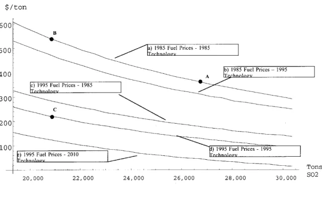
How important are price changes and technical progress in explaining the fall in marginal abatement cost curves? To answer this question, Figure 2 plots estimated marginal abatement cost curves for a generating unit with average Phase I input and output characteristics using (a) 1985 fuel prices and 1985 technology, (b) 1985 fuel prices and 1995 technology, (c) 1995 fuel prices and 1985 technology (d) 1995 fuel prices and 1995 technology and (e) 1995 fuel prices and 2010 technology. In all five curves, output as well as all non-fuel input prices are held constant. The effect of technological improvements, represented by the vertical distance between curves (a) and (b) accounts for about 20 percent of the change of the MAC function, or a decline of about $50 per ton between 1985 and 1995. The effect of changes in fuel prices, represented by the vertical distance between curves (b) and (d) accounts for the remaining 80 percent of the fall in the marginal abatement cost function, a decline of about $200 per ton.
average high sulfur coal price in our dataset is lower than the national average.
100 110 120 130 140 150 160 170 180 190 200 1985 1986 1987 1988 1989 1990 1991 1992 1993 1994 1995 CENTS/MMBTU Sample Average Low Sulfur Coal Price
Sample Average High Sulfur Coal Price
National Average Low Sulfur Coal Price
National Average High Sulfur Coal Price
This figure also demonstrates why marginal abatement costs computed at the plant’s actual level of emissions have fallen even as emissions have themselves declined. Without technological change or changes in fuel prices, an average plant would move in the figure from point A in 1985 to Point B in 1995 (from approximately 27,000 to 21,000 tons of SO2). Its
MAC would increase from approximately $360 per ton of SO2 abated to $540 per ton of SO2
abated, as emissions were reduced. With changes in fuel prices and technology, however, the unit actually moves from point A to Point C, where its marginal abatement cost is only about half as large as it was originally.28 If the current trend in technological improvements continues until the year 2010, this average unit's marginal abatement cost will fall by an additional $100 per ton ((d) to (e)).
FIGURE 2: THE EFFECT OF CHANGES IN FUEL PRICES AND TECHNICAL CHANGE ON MARGINAL ABATEMENT COST FUNCTIONS
28 It is important to keep in mind that the relative importance of technological change and fuel prices on an
individual unit's marginal abatement cost function depends greatly on where in the United States the unit is located. Generating units located in areas that have had access to relatively inexpensive low-sulfur coal for some time would not see a substantial drop in their marginal abatement cost functions due to changes in coal prices.
IV. THE LEAST-COST SOLUTION AND POTENTIAL GAINS FROM TRADE IN THE LONG RUN
A. Preferred Estimates of the Least-Cost Solution
To estimate potential gains from allowance trading in the long run, we use our
econometric estimates to compute the least-cost solution to achieving the SO2 cap in the year 2010. This requires that we make assumptions about parameters that will shift the marginal abatement cost functions over time—the rate of growth of electricity production (Q), the future path of fuel prices (pls and phs), and the rate of technical progress. We must also determine the rate at which coal plants in existence in 1995 will be retired from service, and what SO2 emissions
would have been in 2010 in the absence of the CAAA. The assumptions we make about these parameters are applied consistently across all scenarios we compare.
Electricity Output
We assume that electricity production averaged over all coal-fired units increases at the rate of 1.49% per year.29 Output is, however, likely to increase more rapidly at scrubbed units, which we assume will be utilized at 80 percent of capacity by 2010.30 This fixes the emissions of scrubbed units in the long run. We allocate remaining generation and emissions under the cap to fuel switching units.
Input Prices and Technical Change
In parameterizing the marginal abatement cost functions of fuel switching units, we assume that the real prices of high- and low- sulfur coal remain at 1995 levels and that the rate of technical change experienced between 1985 and 1994 continues through 2010.31
29 EPRI (1997) assumes annual increase in generation from coal-fired facilities of 1% per year through 2005 and flat thereafter; EPA (1995) assumes an average annual increase of 1.3% for thirty years; US EIA (1996) assumes increase in coal-fired generation of 1.1% annually through 2015, but this estimate is revised in US EIA (1997) to 1.49%.
30 Utilization rates at scrubbed units have been increasing over time. There were 28 generating units with retrofit scrubbers in place by the beginning of 1995. The highest utilization rate in 1995 was 88%, and four were above 80% utilization.
31 The fuel price assumption is consistent with the US EIA (1996), while US EIA (1997) revised the forecast to indicate the sulfur premium would shrink slightly further.
Retirement of Coal-Fired Power Plants
We assume 11 gigawatts (GW) of coal-fired capacity in place in 1995 will be retired by the year 2010 and all of that coal-fired capacity will be replaced by natural gas.32 Economic decisions not directly related to the CAAA are the primary determinant of the timing and
decision to switch to natural gas. This will reduce the emissions of these units to negligible levels, thus freeing up allowances and reducing compliance costs for units that remain in the market. Baseline Emissions
We compute baseline emissions—those that would have prevailed absent Title IV—using 1993 emissions rates applied to 2010 levels of electricity production. We assume the declines in emission rates that occurred between 1985 and 1993 were primarily the result of decreases in the price of low sulfur coal and would have happened in the absence of Title IV.33
Continuous Emissions Monitoring Data
An important feature of the 1990 CAAA is that SO2 emissions must be measured by a
continuous emissions monitoring system (CEMS) rather than being estimated based on fuel consumption. Previous studies all use engineering estimates of SO2 emissions. A comparison of
the two measurement techniques reveals that, in 1995, CEMS emissions were about 7 percent higher than estimated emissions, implying that the SO2 cap is effectively 7 percent below the cap
based on engineering formulas. To be consistent with actual practice, we use CEMS data. Minimum Compliance Costs in the Preferred Case
Under the above assumptions, the minimum annual cost of achieving the SO2 cap of 8.95 million tons in 2010 is $1.04 billion (1995 dollars). Of this total, $380 million represents the cost incurred by plants that fuel switch, which account for about 60% of reductions from baseline emissions.34 The other 40% of reductions come from plants that have built scrubbers. For plants that have installed scrubbers, annualized capital costs are $382 million per year and variable costs $274 million per year. No retrofit scrubbers in addition to those constructed in Phase I, which are assumed to be built under all scenarios, are found to be economic in the least-cost solution.
32 The US EIA (1997) predicts that 22 GW of coal-fired capacity will be retired between 1995 and 2010. Given recent experience with coal plant life extension and developments in monitoring technology that have lowered maintenance costs (Ellerman 1998), we expect substantially fewer coal plants to actually retire over that 15 year horizon.
33 Emission reductions before 1995 were not bankable, so there is no reason why fuel-switching plants would reduce their emissions in 1990-1993 to comply with Title IV. In 1994, however, modifications to existing equipment were made to prepare for compliance in 1995 (Ellerman and Montero, 1998).
34 We have investigated the implied change in the transportation of low-sulfur coal between the least-cost solution and present activity. We find it to be a modest extension of recent trends in the increased use of low-sulfur coal.
The marginal cost of emissions reduction, which should approximate the long-run permit price, is $291 per ton of SO2. This assumes that the marginal ton of SO2 is reduced via fuel switching, an assumption that is justified if one compares the cost of reducing SO2 by installing retrofit scrubbers with the cost via fuel switching. Though the useful life of a retrofit scrubber is likely to be close to 20 years (EPA, 1995), the investment decision should reflect current
financial and regulatory uncertainties in the industry, which call for a 10 year payback life (EPRI, 1997). With this decision rule, the average cost per ton of reducing SO2 through additional
retrofit scrubbers is $360. Since this exceeds the marginal cost of SO2 reduction via fuel switching, there is no reason why the marginal generating unit would scrub emissions.
B. Comparisons and Sensitivity Analyses
Table 2 reports sensitivity analyses for our long-run cost estimates, and compares our costs with two previous EPA estimates. The first column reports estimates of costs under command and control (a uniform emission rate standard). The second reports costs under the least-cost solution. The third and fourth columns report marginal and average cost per ton of abatement in the least-cost solution. The fifth column reports the potential gains from trade (the difference between columns one and two).
Our preferred estimate of annual CAAA compliance costs of $1.04 billion per year is far lower than EPA predicted when the 1990 Clean Air Act Amendments were drafted (EPA 1989, 1990). In fact, it is less than half EPA’s estimates of the costs of the trading program, which are reported at the bottom of Table 2 in the fourth and fifth rows. This raises two questions: Is our estimate of compliance costs biased downward? If not, why is it so much lower than EPA’s original estimates of such costs?
The assumptions made above with regard to electricity generation and fuel prices are likely to overstate, rather than understate costs. We assume, for example, the same rate of growth in electricity generated by coal, and a slower rate of retirement of coal-fired plants than official predictions (U.S. EIA, 1997). The assumption that high- and low- sulfur coal prices remain at their 1995 level is also conservative—the Energy Information Administration (1997) predicts a reduction in the low-sulfur premium below 1995 levels.
The one assumption that might bias our cost estimates downward is our assumption that technical progress will continue from 1995 until 2010 at the same rate as between 1985 and 1994. If we assume, at the other extreme, that technical progress stops in 1995, our estimate of
compliance costs rises to $1.51 million (1995 dollars), and our estimate of long-run allowance price rises to $436 per ton of SO2 (see row 2 of Table 2). Even this extreme assumption puts our estimate of total compliance costs below EPA’s (1990) estimate of $2.3 - $5.9 billion (Table 2), and our estimate of marginal cost ($436) below EPA’s estimate of $579-$760 per ton.35
35 Recent engineering studies that acknowledge the use of low-sulfur coal for compliance have also identified the declining trend of marginal and annual total costs of compliance (EPA (1995) and EPRI (1995,1997)).
TABLE 2: LONG-RUN (PHASE II, YEAR 2010) COST ESTIMATES (1995 dollars) (1) Total Cost under "Enlightened " Command and Control (billions) (2) Total Cost under Efficient Trading (billions) (3) Marginal Cost per Ton SO2 ($/ton) (4) Average Cost per Ton SO2 ($/ton) (5) Potential Gains from Trade (billions) Preferred Estimate 1.82 1.04 291 174 0.78 1995 Technology 2.23 1.51 436 198 0.72 1989 Prices and 1989 Technology 2.67 1.90 560 236 0.77 EPA (1990) - 2.3-5.9 579-760 299-457 -EPA (1989) - 2.7-6.2 377-511
-It is important for two reasons to understand why these estimates differ. One is to see whether there is a systematic tendency (ex ante) to over-estimate the cost of environmental regulations. That costs are systematically over-estimated has been alleged both by economists and environmentalists (Goodstein and Hodges, 1997; Harrington et al. 1999), and is an especially timely issue in light of debates over the cost of reducing greenhouse gases.
The second reason is that the factors that explain why estimates of compliance costs have fallen also explain why the costs of command and control approaches to reducing SO2 have fallen, and why the potential gains from allowance trading are also lower than originally
anticipated. One reason for EPA’s high estimates of compliance costs could be failure to foresee the continued fall in the low-sulfur coal premium, as well as continuing technical progress in fuel switching.36 To estimate the potential magnitude of these effects, we re-compute the least-cost solution using 1989 prices and technology.37 Columns 2 and 3 of the third row of Table 2 show that both total costs and marginal abatement costs rise by about 90% (relative to our "preferred” estimates in the first row). Total costs rise from $1.04 billion to $1.90 billion and marginal abatement costs rise from $291 to $560. When fuel switching determines the marginal cost of
36 We cannot assert this with certainty since assumptions regarding coal prices and changes in technology are not transparent in EPA 's reports (1989, 1990).
37 We also assume that emissions are estimated based on fuel consumption, as they were in studies prior to the passage of Title IV.
compliance, using 1989 fuel prices and technology can produce marginal cost estimates
approximately as large as those which were predicted when Title IV was written ($579-$760; see column 3 of Table 2). Total costs also increase, in part because a higher sulfur premium lowers the percent of emissions reductions that can be obtained for free. Under our preferred scenario 57 percent of emissions reductions from plants that fuel switch are obtained by realizing negative marginal abatement costs (switching to cheaper low-sulfur coal). This figure, however, falls to 21 percent using 1989 prices and technology.38
Failure to foresee changes in prices and technical progress, however, does not explain all of the difference in total cost estimates. Also important are differences in the baseline from which emissions reductions are measured. In all of our calculations, we assume that the emission rates (lbs. of SO2/mmBtu) that would have prevailed in the absence of the 1990 Clean Air Act
Amendments are those that prevailed in 1993. These are much lower than 1989 emission rates, hence the reductions in emissions necessary to achieve the 8.95 million ton cap, by our
calculations, are much lower than imagined in 1989 (specifically, about 2 million tons lower). Holding MAC curves constant, lowering the necessary reduction in emissions will lower total compliance costs.
Finally, EPA’s estimates of total compliance costs are higher than ours because they assumed that more retrofit scrubbers would be built (37) than were actually constructed (28). They also failed to foresee a 50% fall in the cost of scrubbing that we identify.
C. Potential Gains from Trade
We now consider the cost of meeting the SO2 cap using a command and control approach,
and compute the potential gains from trade as the difference between this cost and the cost of compliance under the least-cost solution. We first model command and control as a uniform performance standard that is designed to achieve the same level of emissions as the trading program, consistent with the goal of Title IV to achieve an average emissions rate of 1.2 pounds of SO2 per million Btu of heat input.39
For our preferred case, we estimate the potential gains from trade compared to the
"enlightened" command and control scenario to be $784 million (43% of the cost of command and control). The potential gains from trade are estimated by subtracting the total costs under
efficient trading in column 2 of Table 2 ($1.04 billion) from the total costs under a command and control program in column 1 ($1.82 billion). While these gains constitute 43% of the cost of
38 While this 57% estimate may seem high, we have evidence from 1995 and 1996 that utilities are realizing such economic cost savings. In 1995 one-quarter of a potential $443 million in savings from fuel switching were realized. In 1996, half of $644 million in potential savings were realized. We believe that increased competition in the electric utility industry will motivate generators to take advantage of these savings.
39 The uniform emission rate standard does not take into account the fact that some units may face unrealized "economic" emission reductions beyond those mandated by the standard. Therefore, emissions are lower under the uniform standard than they are under a trading program, which provides firms with higher abatement costs the flexibility to capture the slack in the effective emission constraint at other firms (Oates, Portney and McGartland 1989). It should be noted that if a uniform emission rate is set so that total emissions under a trading program equal those under a uniform emission rate standard, it will still be the case that costs under the trading program will be less than under a uniform emission standard. Potential gains from trade will be lower, however.
command and control, they are not as large as were originally predicted. The GAO (1994), for example, estimated that a command and control cap on emissions at each generating unit would cost approximately $5.3 billion annually and that the reduction in costs from efficient trading would be $3.1 billion (about 60% of the command and control figure).
The explanation for our more modest estimates of trading gains is clear—the factors that have caused marginal abatement costs to fall also would have lowered the costs of achieving the SO2 emissions cap via command and control. These include the fall in the price of low sulfur coal
and, to some extent, technical improvements that have facilitated fuel switching.40 It should also be noted that, in addition to lowering marginal abatement cost curves (see Figure 2), the fall in low sulfur coal prices has made marginal abatement cost curves more homogenous. This is because the cost of transporting low sulfur coal to more distant locations, for example, the East and Southeast, has fallen, rendering differences in transportation cost a less important component of the overall cost of fuel switching. Since a major source of trading gains is differences in
marginal abatement cost curves among units in the market, this increased homogeneity is also partly responsible for low gains from trade.
One alternative to our preferred assumptions is the possibility that, in the absence of the cap and trading program, a different command and control policy would have been adopted. In place of our “enlightened” command and control policy of an emission rate performance standard, we considered the possibility of forced retrofit scrubbing to achieve an equivalent level of
aggregate emissions. We assume the cost per ton of additional retrofit scrubbing to be the same as that observed for retrofit scrubbers built in Phase I.41 The aggregate cost of this approach would have been $2.6 billion per year. Compared to this alternative, the trading program generates potential cost savings of $1.6 billion ($2.6 - $1.04 billion). About half of these savings are
captured by moving from forced scrubbing to a more flexible uniform performance standard ($2.6 - $1.82 billion = $780 million).
The relatively modest potential gains from trading relative to a more flexible uniform performance standard ($784 million) should not be interpreted as a criticism of the allowance market, but they are likely to have an impact on market performance. If potential gains from trade are small and transaction costs of using the market are substantial, utilities will be less eager to trade allowances. In the next section, we analyze the performance of the SO2 allowance market
in 1995 and 1996 to determine both the potential gains from trade under a perfectly functioning market and how much of these gains actually have been realized.
40 Some of the technological developments in fuel blending may not have occurred under a uniform emissions standard since blending of coals with different sulfur contents by itself (i.e. without the option of purchasing allowances) generally would not be sufficient to achieve the required emission reductions. Similarly, there would have been less incentive to improve the performance of scrubbing equipment under a uniform CAC emission rate standard, and the witnessed improvements may not have been realized. To the extent that the effects of the
allowance trading program on technological change in emissions reduction are reflected in our data, our estimates of the costs of a uniform emission rate standard and the potential gains from trade are likely understated.
41 That is, we assume a 20 year depreciation schedule with a historic cost of capital, which was applicable to retrofit scrubbers initiated before the start of Phase I. These assumptions result in a lower cost of scrubbing than were we to assume that some of these scrubbers would be built after 1995, when a higher cost of capital for the industry would be applicable.
V. THE PERFORMANCE OF THE ALLOWANCE MARKET IN 1995 AND 1996
In 1995, the aggregate emissions of Phase I units were approximately 5.3 million tons, rising to 5.44 million tons in 1996. To compute the least-cost method of achieving these emissions levels, we parameterize marginal abatement cost functions for each unit using actual output levels and input prices. Technical progress is assumed to occur at the same annual rate as observed between 1984 and 1995. We take as our baseline 1993 emission rates, which we apply to 1995 and 1996 electricity generation to predict emissions in the absence of Title IV.
The least-cost solution yields a common marginal abatement cost (for the last ton emitted by all units that fuel switch) and a set of efficient emission levels for all generating units. To compute total costs, we integrate each unit’s marginal abatement cost curve from baseline emissions to emissions under the least-cost solution. The total cost of actual emissions in each year is computed analogously, except that integration under the MAC curve occurs from baseline emissions to actual 1995 and 1996 emissions.42
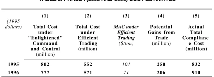
TABLE 3: PHASE I (1995 AND 1996) COST ESTIMATES
(1995 dollars) (1) Total Cost under "Enlightened" Command and Control (million) (2) Total Cost under Efficient Trading (million) (3) MAC under Efficient Trading ($/ton) (4) Potential Gains from Trade (million) (5) Actual Total Complianc e Cost (million) 1995 802 552 101 250 832 1996 777 571 7 1 206 910
The first row of Table 3 suggests that the allowance market did not realize potential gains from trade in 1995. The estimated annual command and control cost of achieving 1995 emissions is $802 million (1995 dollars) as shown in the first column of row 1. The estimated cost with efficient trading is $552 million as shown in column two, hence, the potential gains from trading are estimated to be $250 million. The fifth column reports the estimated actual cost of achieving 1995 emissions to be $832 million.43 The difference between the costs under efficient trading and actual compliance costs is $280 million, suggesting that potential cost savings were
42 Emission rates are based on DOE-EIA engineering estimates, not CEMS data. Because both the heat input and SO2 emissions estimated by the DOE-EIA are lower than the CEMS measurements, the estimated emission rates
under DOI-EIA and CEMS are equal to each other on average.