Financing constraints, firm level adjustment of capital and aggregate implications

Financing constraints, firm level adjustment

of capital and aggregate implications

Ulf von Kalckreuth

Discussion Paper

Series 1: Economic Studies

No 11/2008

Editorial Board: Heinz Herrmann

Thilo Liebig

Karl-Heinz Tödter

Deutsche Bundesbank, Wilhelm-Epstein-Strasse 14, 60431 Frankfurt am Main, Postfach 10 06 02, 60006 Frankfurt am Main

Tel +49 69 9566-1

Telex within Germany 41227, telex from abroad 414431 Please address all orders in writing to: Deutsche Bundesbank,

Press and Public Relations Division, at the above address or via fax +49 69 9566-3077

Internet http://www.bundesbank.de

Reproduction permitted only if source is stated. ISBN 978-3–86558–426–7 (Printversion) ISBN 978-3–86558–427–4 (Internetversion)

Abstract:

Following a positive shock, financing constraints will prolong or impede economic ex-pansion that would have been optimal in an unconstrained environment. The study of dynamic adjustment therefore offers a direct way of verifying the presence of financing constraints and assessing their consequences for economic allocation.

This paper compares the speed of adjustment of constrained and unconstrained firms using categorical information from survey data on the restrictions under which adjust-ment takes place. A set of moadjust-ment conditions for the use in GMM estimation is devel-oped, to cope with the problem of time varying speed of adjustment when the target level is partially unobserved.

After estimating the micro-dynamics of capital demand, I show that the changing com-position of the population makes for a time-varying sensitivity of the aggregate with respect to macroeconomic shocks.

Keywords: Financing constraints, adjustment, dynamic panel data models JEL-Classification: C23, D21, D24

Non technical summary

With informational frictions, indivisibilities and irreversibilities, the reaction of aggre-gate factor demand to aggreaggre-gate shocks will not be time-invariant. Instead, it will de-pend on the distribution of individuals. If many individuals are in a state that allows or enforces sharp reactions, then aggregate shock sensitivity is marked. There is a high value attached to direct information on the position of individuals in state space that would allow us to infer the aggregate sensitivity.

This paper argues that survey data can be a timely and useful source of information about the relevant constraints for individuals. More specifically, it deals with financing constraints at the firm level and their effect on the aggregate.

I argue first that the most important real effect of financing constraints is to slow down the adjustment of capital and labour input to positive, expansionary shocks. I then lay out a GMM based technique to estimate micro level adjustment equations when the tar-get is unobserved and the adjustment speed varies over time, and categorical informa-tion on adjustment regimes is available. The empirical work is based on micro data from a survey on the investment behaviour of German industrial companies (the Ifo Investi-tionstest).

I concentrate on adjustment functions for the real capital stock. The estimates show that regime specific dynamic behaviour can successfully be disentangled. We see that – as hypothesized – financing constraints slow down the speed of adjustment of firms. Fur-thermore, this effect is concentrated on or perhaps even limited to smaller firms. With large firms, no clear speed differential can be detected. The speed of adjustment of small firms is clearly higher than for large firms.

In a last step, some of the aggregate implications are worked out. The aggregate sensi-tivity changes with the composition of the aggregate. With estimated adjustment func-tions in hand, it is easy to trace the time-varying aggregate sensitivity. This offers an important new way in which survey data can be used by analysts and forecasters.

Nicht-technische Zusammenfassung

Wegen informationeller Friktionen, Unteilbarkeiten und Irreversibilitäten ist die Reak-tion der aggregierten Faktornachfrage auf sektorale Schocks im Zeitablauf nicht unver-änderlich. Sie wird vielmehr von der Verteilung der Firmen abhängen. Wenn viele Un-ternehmen sich in einem Zustand befinden, der eine rasche Reaktion erlaubt oder er-zwingt, ist die Sensitivität hinsichtlich expansiver Schocks besonders groß. Aus diesem Grund sind direkte Informationen über die Position der Unternehmen von hohem Wert, da sie einen Aufschluss über die Sensitivität des Unternehmenssektors als Ganzem geben können.

Diese Arbeit stellt heraus, dass Umfragedaten eine wichtige und zeitnahe Informations-quelle hinsichtlich der relevanten Beschränkungen für Individuen sein können. Es wird spezifisch die Bedeutung von Finanzierungsrestriktionen für die Anpassungsgeschwin-digkeit auf der Mikroebene und deren Folgen für das Aggregat behandelt.

Zunächst wird dargelegt, dass der wichtigste reale Effekt von Finanzierungsbeschrän-kungen in einer Verminderung der Anpassungsgeschwindigkeit von Kapital- und Ar-beitseinsatz an positive, expansive Schocks darstellt. Für die empirische Überprüfung dieser These wird eine besondere GMM-Technik beschrieben, welche die Schätzung mikroökonometrischer Anpassungsgleichungen in solchen Fällen erlaubt, in denen das Zielniveau nicht beobachtet werden kann und die Anpassungsgeschwindigkeit über die Zeit variiert, dafür jedoch kategoriale Information über das Anpassungsregime verfüg-bar ist. Die Datengrundlage ist durch Einzeldaten aus einem Investitionssurvey für deut-sche Industrieunternehmen, dem Ifo-Investitionstest, gegeben.

Es werden Anpassungsfunktionen für den Kapitalstock geschätzt. Die empirische Me-thodik erweist sich bei der Rekonstruktion der regimeabhängigen Dynamik als erfolg-reich. Den theoretischen Erwartungen entsprechend senken Finanzierungsbeschränkun-gen die Anpassungsgeschwindigkeit von Unternehmen. Weiterhin zeigt sich, dass dieser Effekt besonders bei kleineren Unternehmen zu beobachten ist oder vielleicht sogar auf diese beschränkt ist. Außerdem wird sichtbar, dass die Anpassungsgeschwindigkeit kleiner Unternehmen im Allgemeinen deutlich höher ist als die großer Unternehmen.

Schließlich werden die Konsequenzen für das Aggregat entwickelt. Die Sensitivität des Unternehmenssektors als Ganzem ändert sich mit der Zusammensetzung des Aggregats. Mit Hilfe der geschätzten Anpassungsfunktionen ist es leicht, die zeitliche Variation der sektoralen Sensitivität nachzuzeichnen. Dies eröffnet einen wichtigen neuen Weg für die Nutzung von Surveydaten für die ökonomische Analyse und Prognose.

Contents

1 Introduction 1

2 Financing constraints and investment dynamics 3

3 State dependent adjustment dynamics with unobserved targets 5

3.1 The estimation problem 6

3.2 A non-linear transformation 7

4 Empirical strategy 9

5 Descriptive statistics and estimation results 12 6 Aggregate implications of adjustment heterogeneity 16

Lists of Tables and Graphs

Table 1 Descriptive statistics for continuous variables 21

Table 2 Breakdown by firm size classes 21

Table 3 Financing and sales conditions for realised investment: Tabulations and panel variation

22

Table 4 Transition matrix for regime partition R(2) 22 Table 5 Transition matrix for regime partition R(3) 23 Table 6 Adjustment speed according to financing conditions

Regime partition R(1), 5 regimes, based on factors for realised investment

24

Table 7 Adjustment speed according to financing conditions Regime partition R(2), 3 regimes, based on factors for realised investment

25

Table 8 Adjustment speed according to financing conditions and expansion mode

Regime partition R(3), 3 regimes, based on lagged factors for expected investment

26

Graph 1 Time varying sensitivity of capital demand (for Regime Partition R(3), Table 8, Column I)

Financing constraints, firm level adjustment of capital

and aggregate implications

*

1. Introduction

With informational frictions, indivisibilities and irreversibilities, the reaction of aggre-gate factor demand to aggreaggre-gate shocks will not be time-invariant. Instead, it will de-pend on the distribution of individuals in the relevant state-space. In a prototypical (S,s) model of irreversible investment, a region of inaction is bounded by an upper and a lower threshold that triggers investment and hiring, or disinvestment and firing.1 The individual reaction to measures of fundamentals will be nonlinear: investment bursts (spikes) will be followed by relative inaction. On the aggregate level, the reaction to a positive shock will be sharp if a large mass of individual agents is situated near the up-per threshold, as opposed to a situation where a series of negative shocks has driven agents to the edge of disinvestment.2 Models of informational asymmetry describe a similar range of inactivity for individuals. If the market value of their assets is insuffi-cient to sustain externally financed expansion, firms will not be able to make use of profitable investment opportunities, or have to take the slow lane of accumulation by internal finance. Again, the sensitivity of aggregate factor demand to productivity or demand shocks and user cost changes induced by tax reforms or monetary policy will depend on the distribution of equity or liquidity ratios among firms, as induced by re-cent history. The action of the financial accelerator is quite asymmetric in booms and busts.3 This "asymmetry", as we may call the state dependence of correlations between

* _{Correspondence: Ulf von Kalckreuth, Deutsche Bundesbank, Research Centre, Wilhelm Epstein-Str.}

14, 60431 Frankfurt, Germany. E-mail: ulf.von-kalckreuth@bundesbank.de, Website: http://www.von-kalckreuth.de

Disclaimer: The views expressed in this paper do not necessarily reflect those of the Deutsche Bundesbank. All errors, omissions and conclusions remain the sole responsibility of the author.

Acknowledgements: This paper was written for presentation at the Spring Conference 2007 "Mi-crodata Analysis and Macroeconomic Implications", organised by the Deutsche Bundesbank and the Banque de France, Eltville, 27 and 28 April 2007. A nascent version was presented even before on the Conference in Honour of George von Fürstenberg, on 28-29 April 2006 at Indiana University in Bloomington. In January 2008, it was given at the NAEFA meeting in New Orleans. I received valu-able comments by the respective discussants, Vassilis Hajivassiliou, Greg Udell and George Hall. Repeated interactions with Jörg Breitung sharpened my view on the econometrics, and I received important feedback and advice from George von Furstenberg on the economics of the paper. A comment by Olympia Bover led to a major change in the estimation strategy. Thanks also to Ben Craig, Heinz Herrmann and Wolfgang Lemke for helpful discussions.

1 _{Abel and Eberly (1996), Abel, Dixit, Eberly and Pindyck (1996), Bentolila and Bertola (1990).}

2 _{Caballero, Engel and Haltiwanger (1995, 1999).}

3 _{See Bernanke and Gertler (1989, 1995) and Bernanke, Gertler and Gilchrist (1996, 1999) on the credit}

macroeconomic aggregates and prices, is important for policy makers as well as for market participants, forecasters and analysts.

In such a situation, there is a high value attached to direct information on the position of individuals in state space that would allow us to infer the aggregate sensitivity. This paper argues that survey data can be a timely and informative source of information about the relevant constraints for individuals. More specifically, it deals with financing constraints at the firm level and their effect on the aggregate.

I argue first that the most important real effect of financing constraints is to slow down the adjustment of capital and labour input to positive, expansionary shocks (Section 2). In explicitly relating financing constraints to the adjustment dynamics, our paper is related to Basu and Guariglia (2002), von Kalckreuth (2006) and Bayer (2006). I then lay out a GMM based technique to estimate micro level adjustment equations when the target is unobserved and the adjustment speed varies over time, and categorical infor-mation on adjustment regimes is available (Section 3). This estiinfor-mation technique is developed in a companion paper, von Kalckreuth (2008), and it has a wide range of ap-plications for other important adjustment processes, such as sales price adjustment by firms, interest pass through by banks or the adjustment of equity ratios. The specific empirical strategy for the problem at hand is developed in Section (4). Section (5) takes the estimation technique to the data, using micro data from a survey on the investment behaviour of German industrial companies (the Ifo Investitionstest). Adjustment func-tions for the real capital stock are estimated. These estimates show that regime specific dynamic behaviour can successfully be disentangled. We see that – as hypothesized – financing constraints slow down the speed of adjustment of firms. Furthermore, this effect is concentrated on or perhaps even limited to smaller firms. With large firms, no clear speed differential can be detected. Ultimately we see that the speed of adjustment of small firms is clearly higher than for large firms. The results fit extremely well to what was obtained by von Kalckreuth (2006) for capacity adjustment of UK firms, us-ing an entirely different methodology on a different type of data.

In a last step, some of the aggregate implications are worked out (Section 6). The ag-gregate sensitivity changes with the composition of the agag-gregate. With estimated ad-justment functions in hand, it is easy to trace the time-varying aggregate sensitivity. This offers an important new way in which survey data can be used by analysts and forecasters.

2. Financing constraints and investment dynamics

Empirical work on financing constraints has traditionally been based on an approach pioneered by Fazzari, Hubbard and Peterson (1988). They divide their sample into con-strained and unconcon-strained firms using ad hoc criteria. If the investment of financially constrained firms shows a higher sensitivity to internal finance than the investment of their unconstrained counterparts, this is seen as evidence for the existence of binding fi-nancial constraints. In recent years, this approach has been forcefully criticised. Kaplan and Zingales (1997) state that there is no theoretical reason why – in a comparison be-tween firms – a larger cost differential bebe-tween internal and external finance might lead to a higher cash-flow sensitivity, as opposed to just comparing the extreme cases of a constrained firm and an absolutely unconstrained one. A non-monotonic relationship between the cost differential and excess sensitivity is perfectly conceivable.4 On the other hand, it has been shown theoretically that, under certain conditions, cash flow terms can be significant even in the absence of financing constraints.5 Ultimately, there is a pervasive missing variable problem. Cash flow is a close relative to profit, a sum-mary measure of all that is important for a firm, and it is useful in predicting future values of variables relevant to the current investment decision.6

Here, we use a direct approach by relying on explicit statements by the firms them-selves. We are able to explore the micro data base of the Ifo institute’s Investitionstest

(Investment Test, IT) for the manufacturing sector in West Germany during the years 1988 to 1998. During these eleven years, the autumn wave of the survey yields 25,643 observations on a total of 4,443 firms, with 2,331 firms per year on average. Apart from its size and coverage, the data set has two important characteristics that are relevant to our problem. First, it contains many small firms, on which very little information is available in data sets based on quoted companies. Although large firms are clearly over-sampled, almost one half of the IT observations refer to firms with fewer than 200 em-ployees, and around 20% of the firms have fewer than 50 employees. Second, the data set contains information on financing constraints that firms face in their investment de-cisions. Notably, a number of firms (around one quarter of respondents) explicitly state that their investment demand is limited by the cost and/or the unavailability of finance. Although part of this may be due to the workings of the classical interest rate channel,

4 _{The discussion was continued in Fazzari, Hubbard and Peterson (2000) and Kaplan and Zingales}

(2000).

5 _{See the models by Abel and Eberly (2003), Cooper and Ejarque (2001), and Gomes (2001).}

these aggregate effects can be eliminated by the use of time dummies, focussing on differential changes in time.

Von Kalckreuth (2004) argues that a specific pattern with respect to the distribution of investment over time should be expected to hold for financially constrained firms. Given a shock, an unconstrained investor can adapt rapidly or even instantaneously if other types of adjustment costs are unimportant. The bulk of investment spending will take place in the first few periods, and there may be a spike in the first period. If the investor is financially constrained, however, marginal costs of finance will increase with the amount of spending, possibly to infinity. In such a setting, the investor has to equal-ise marginal costs of finance and the marginal value of new investment in each period. After an initial debt-financed increase in the capital stock that leads to a worsening of the financial position, the firm needs internal finance to continue the expansion and to repair balance sheets gradually. Thus, the adjustment will be spread over time. This cru-cial difference in the adjustment dynamics can be used to identify financru-cially con-strained firms, or better, to test whether a subset of supposedly concon-strained firms really is, without having to take recourse to cash flow sensitivities. The hypothesis is exam-ined empirically by von Kalckreuth (2006), using set of survey data on UK firms with entirely qualitative information. The duration of capacity restrictions is compared be-tween firms that characterised themselves as being financially constrained, and others that did not.

The Ifo Investment Test has a different and more specific informational content, in that many key variables are continuously scaled, so that the adjustment dynamics can be much more closely observed. Von Kalckreuth (2004) proceeds to sort firms into two groups, according to whether they are predominantly financially constrained or not. This approach has a serious drawback: it does not make use of the time variation in the financing constraints variable for a given firm.7 This is most valuable in micro-econometrics, when many important aspects of the process in question are unobserved, but can be trusted to be relatively stable in time. It is the variation in the left hand vari-able following a variation of the explanatory varivari-able that helps to identify structural relationships. However, a time varying adjustment coefficient poses special problems if the target is unobserved. These will be discussed in the next section.

The interrelation of financing constraints and investment behaviour is studied also by Basu and Guariglia (2002), looking at the dynamics of capital returns. Our approach is

closest in spirit to Bayer (2006). In this paper, a gap model of adjustment is estimated, where capital imbalances are measured as an imputed difference between capital stock and imputed target, whereas financing constraints are proxied simply using the equity ratio. For both of these fundamental magnitudes, a treatment of unobserved differences between firms is extremely difficult. Therefore, the empirical approach presented next may greatly alleviate some of these measurement problems.

3. State dependent adjustment dynamics with unobserved targets

This section draws on von Kalckreuth (2007), a companion paper that studies moment conditions that can be used in the estimation of an adjustment model with unobserved target and time-varying speed of adjustment in a context of panel data. The econometric method is tailor-made for the problem at hand, but has considerably more general use. In a rather general form, economic adjustment can be framed by a "gap equation", as formalised by Caballero, Engel and Haltiwanger (1995):

(

)

, ,, , , i t i t i t i t y x x Δ = Λ z ⋅ , where * , , 1 , i t i t i t x = y ₋ −y .

Here, subscripts refer to individual i at time t, and x_{i t,} is the gap between the state y_{i t, 1−}

inherited from the last period and the target * ,

i t

y that would be realised if adjustment costs were zero for one period of time. The speed of adjustment, written as a function Λ of the gap itself and additional state variables z_{i t,} , determines the fraction of the gap that is removed within one period of time. The adjustment function reflects convex or non-convex adjustment costs, irreversibility and indivisibilities, financing constraints or other restrictions, and the uncertainty of expectation formation. With quadratic adjust-ment costs or Calvo-type probabilistic adjustadjust-ment, Λ will be a constant.

Estimating the function _Λ is inherently difficult. In general, both * ,

i t

y and x_{i t,} are not observable. However, some measure of the gap is needed for estimation, and if Λ explicitly depends on x_{i t,} , the measure moves to the centre stage.

In linear dynamic panel estimation, this problem can successfully be addressed by pos-iting an error component structure for the measurement error and eliminating the indi-vidual fixed effect by a suitable transformation, such as first differencing. See Bond et al. (2003) and Bond and Lombardi (2007) for an error correction model of capital stock adjustment. The GMM estimator developed by Arellano and Bond (1991) accounts for the presence of lagged endogenous variables, the endogeneity of other explanatory

variables, and unobserved individual specific effects. Individual effects (including a possible measurement error in the target) are differenced out. Endogenous explanatory variables can be instrumented using lagged dependent variables if serial correlation of the error process is limited. Time fixed effects can also be accommodated; the remain-ing idiosyncratic component of the measurement error needs to be uncorrelated with the instruments.

In the unrestricted, non-linear case, this approach is not feasible, as a host of incidental parameters will threaten identification. But there may be direct qualitative information on the level of Λ

( )

, e.g. from survey data, ratings or market information services. If one is willing to treat the adjustment process as piecewise linear, distinguishing regimes of adjustment, then this information can be harnessed to eliminate the incidental pa-rameters from the problem completely.

3.1. The estimation problem

I examine a situation where a variable y_{i t,} reverts to some target level * ,

i t

y characteristic of individual i. The speed of adjustment depends on the value of r_{i t,} . This is an L -dimensional column vector of regime indicator variables, with one element taking a value of 1, and all others being zero. The equation is:

(

)

(

*

)

, 1 , 1 , 1 , , i t i t i t i t i t y _{α −} y ₋ y _ε Δ = − − − + , with , ' , i t i t α =α r .

The target level * ,

i t

y is unobservable. It follows an equation that contains an individual-specific latent term:

* '

, ,

i t i t i

y =x β+_μ .

The vector x_{i t,} may encompass random explanatory variables, deterministic time trends and also time dummies. In its absence, the target level is entirely unobservable, but static. The idiosyncratic component _μi in the adjustment equation may reflect a measurement error or unobserved explanatory variables. Vector α holds the state dependent adjustment coefficients. The adjustment coefficient _{αi t,} varies over time and individuals, and

(

1−_{αi t, 1−}

)

is the adjustment speed at date t. The regime variable r_{i t,} is generated by a threshold process:

(

)

, 1 ,

( )k _{i t} =Ind c_k− ≤s_{i t} ≤c_k

r ,

with s_{i t,} some latent variable. In general, a non-zero covariance between the error term and the regime indicators, cov

(

_{εi t,},r_{i t,}

)

≠0, can be expected. However, we assume that

, 1 ' , 1

i t i t

α − =α r − is predetermined with respect to εi t, , or more exactly:

(

, , 1 , 2 , , 1 , 1 , 2 0

)

E _{εi t} r_{i t−} ,r_{i t−} , ,_K x_{i t k−} ,x_{i t k− −}, ,_{K εi t k− −} ,_{εi t k− −} , , ,_{K μi} y_i =0 for some k∈

{

1, 2,K

}

.

As we do not observe the target, we have no direct information on the position of the individual relative to the target. But the panel dimension can help us to identify the ad-justment process nonetheless, as it allows us to use an error component approach for modelling the unobserved target. In the adjustment equation, both the individual effect and x_{i t,} are interacted with a time varying and endogenous variable.

3.2. A non-linear transformation Solving for y_{i t,} yields:

(

)

'

(

)

, , 1 , 1 , 1 , , 1 , latent process 1 1 i t i t i t i t i t i t i i t y =_{α −} y ₋ + −_{α −} x β+ −_{α − μ ε}+ 1442443. (1)

It is easily seen that, unlike the case of the standard linear dynamic panel model, first differencing will not remove the latent fixed effect _μi from the equation:

(

)

(

)

'

(

)

(

)

, , 1 , 1 , 1 , , 1 , latent process ' 1 ' i t i t i t i t i t i t i i t y ₋ y ₋ ⎡ _{α −} ⎤ _{−μ ε} Δ = Δα r + Δ_⎣ − x _⎦β+ −1 α Δ r + Δ 14444244443.

Von Kalckreuth (2008) develops a nonlinear transformation that eliminates the unob-served heterogeneity. Holtz-Eakin, Newey and Rosen (1988) propose quasi-differencing as a strategy in a case where fixed effects are subject to time varying shocks that are common across individuals.8 Their method can be modified and generalised to the case at hand, where coefficients are endogenous and vary over time and individuals. Multi-plying equation (1) by

(

1−_{αi t, 2−}

) (

1−_{αi t, 1−}

)

and subtracting the lag of the original adjustment equation leads to

(

)

, 2 ' , , 2 , 1 , 2 , , , 1 1 1 1 i t i t i t i t i t i t i t i t y y α α α ξ α − − − − − − Δ − Δ − − Δ = − x β , with , 2 , , , 1 , 1 1 1 i t i t i t i t i t α ξ ε ε α − − − − = − − .

The unobserved heterogeneity _μi has been eliminated.9 Let d r

(

_{i t, 2−} ,r_{i t, 1−}

)

be an _L2_×1

indicator vector, where each element is a dummy variable indicating one of the possible switches from r_{i t, 2−} to r_{i t, 1−} . Let λ be the vector of coefficients

(

1−_{αi t, 2−}

) (

1−_{αi t, 1−}

)

corresponding to the elements of d

( )

⋅ :

1 1 2 3 2 1 1 1 1 1 ' 1 1 1 1 1 1 L L L L α α α α α α α − α − ⎛ _{− − − −} ⎞ =⎜ _{− − − −} ⎟ ⎝ ⎠ λ _{K K} .

Let ultimately δ be a vector of products of the adjustment coefficients,

(

1−α

)

, and β:

(

)

(

)

(

)

(

)

1 2 1 1 1 _L α α α − ⎛ ⎞ ⎜ ₋ ⎟ ⎜ ⎟ = − ⊗ =_{⎜ ⎟} ⎜ ⎟ ⎜ ₋ ⎟ ⎝ ⎠ β β δ 1 α β β M .

Then we can write:

,

i t

ξ =λ'd r

(

i t, 2− ,ri t, 1−

)

Δ −yi t, α'ri t, 2− Δyi t, 1− −δ'ri t, 2− Δxi t, . (2)

This equation is linear in the transformed variables, but nonlinear in the unknown pa-rameters α and ß. In the companion paper, it is shown that levels y_{i t p k,− −} and x_{i t p k,− −} , as well as regime indicators r_{i t p,− −1}, p=

{

1, 2,K

}

are instruments in equation (2), i.e. the following moment conditions are available for the identification of the unknown pa-rameters:

(

, ,

) (

, ,

) (

, 1 ,

)

E y_{i t p k i t− − ξ} =E x_{i t p k i t− − ξ} =E r_{i t p− −ξi t} =0.

9 _{Applied to the current problem, the quasi-differencing transformation proposed by Holtz-Eakin,}

Newey and Rosen lags equation (1), multiplies both sides by

(

1−_{αi t, 1−}

) (

1−_{αi t, 2−}

)

and subtracts the

result from equation (1). Although this eliminate the fixed effect, in the given context the transformed

error term _{εi t,} − −

(

1 _{αi t, 1−}

) (

1−_{αi t, 2−}

)

_{εi t, 1−} is unsuitable for estimation, as α_{i t, 1}− and εi t, 1− will be

The paper describes in detail how GMM estimation of α and ß is to be implemented, using Gauss-Newton iterations to deal with the nonlinearities involved.

4. Empirical strategy

Following the gap approach, I formulate the econometric model as a partial adjustment mechanism. The model is a special case of the error correction factor demand equation invented by Charles Bean (1981), and introduced to the micro literature by Bond, Elston, Mairesse and Mulkay (2003).10 A full blown ECM that would also take transi-tory dynamics into account could in principle be estimated as well, see von Kalckreuth (2008), Appendix A. In practice it is difficult to separately identify transitory dynamics and overall adjustment speed if all coefficients are regime specific.

The point of departure is the static neoclassical equation for factor demand. Using a constant returns CES production function, the following linear equation for capital results from the first-order conditions of profit maximisation:

* * * *

logK_t =logY_t −_σlogUC_t +logh_t,

where K_t is capital, Y_t is real output, UC_t is the user costs of capital, _σ is the elasticity of substitution, and h_t is a magnitude that depends on technology parameters and the time varying total factor productivity. A star denotes a long-run, equilibrium value. We may model adjustment by replacing the starred values by observed quantities:

*

, ,

logK_{i t} =logS_{i t} + +_{λ μt i}. (3)

Here, _λt is a time fixed effect that catches the effect of user cost changes, time varying total factor productivity and other macro disturbances and will be estimated using a full set of time dummies. The firm fixed effect _μi will catch the unobserved firm specific technological determinants for capital intensity. The log of real sales, logS_{i t,} will be our proxy for variations in real output. Depending on the usage of intermediate products as inputs, real sales and real output will differ, but to the degree that the share of interme-diates in output is a firm specific constant underlying a common trend equation, equa-tion (3) still holds. Assuming that the speed of adjustment may vary with financing con-ditions, we arrive at the following adjustment equation:

( )(

)

, , 1 , 1 , ,

logK_{i t φ i t−} logK_{i t−} logS_{i t λ μt i εi t}

Δ = − r − − − + , (4)

with

( )

i t, 1 1 i t, 1 1 ' i t,

φ r − = −α − = −α r ,

where _φ

( )

r_{i t, 1−} is the time varying, regime specific speed of adjustment and _{αi t, 1−} is a measure of regime specific persistence. In a subset of estimates, the target equation (3) – and the expression in brackets in equation (4) – will be augmented by

, ' ,

i t i t

ω =ω z , (5)

with z_{i t,} a vector of indicators for the levels of the sales conditions in period t, and _{ωi t,} thus giving additional information on the level of the capital stock target.

Question 5 [Autumn survey]: Factors influencing investment in 1999-2000

In 1999-2000 our investment in western Germany was/is being positively/adversely affected by the following factors: (Please refer to the explanatory notes on the reverse of the accompanying letter.)

1999 2000 Factors Very stimu-lating Stimu-lating No influ-ence Lim-iting Very limi-ting Very stimu-lating Stimu-lating No influ-ence Lim-iting Very limi-ting Sales conditions / expectations Availability / costs of finance Earnings expectations Technical develop-ment Acceptance of new technologies Basic economic policy conditions Other factors, namely ...

The Ifo data set and its information on investment and financing conditions have been discussed in detail by von Kalckreuth (2004). In order to generate regime indicators, I use Question 5 of the autumn survey, which asks for factors stimulating or limiting in-vestment in the current year and in the coming year. Both sets of answers are utilised. I generate three different sets of regime indicators. In the data sets, the factors for in-vestment may take one of five values. Our first regime partition, R(1), is defined straightforwardly using the values of the financing factor for realised investment in Question 5. This regime indicator comes very natural and therefore its results will be suggestive. However, it has two drawbacks. First, testing the significance of financing constraints becomes difficult if there are as much as five different regimes. Therefore, a second indicator, R(2) distinguishes only three regimes, by aggregating the categories "very stimulating" and "stimulating" to one regime, and "limiting" and "very limiting" to another.

A potential problem with R(1), shared by R(2), is the requirement that regime informa-tion be predetermined. A shock to the investment equainforma-tion – a large value of _{εi t,} – may lead to financing needs that may themselves bring about a worsening of financial con-ditions. Endogeneity is no problem if firms identify financing conditions in a way that abstracts from current financing needs, but this is hard to verify. I therefore define a third regime partition, R(3), on the basis of factors related to expected investment – the right hand set of categories in Question 5 – lagged one year. The statement on financing conditions thus antedates actual investment expenditure by about one year.11

The regime partition R(3) also deals with another issue. The theoretical argument on financing constraints and the speed of adjustment relate to firms having to finance posi-tive investment expenditures, either expanding the firm or restructuring the capital stock in order to cope with a changing economic environment. It is not clear what is to be expected from firms that aim at downsizing. Furthermore, as has been stated above, the adjustment speed for rapidly downsizing firms may be mismeasured anyway. Therefore R(3) distinguishes three regimes: first, stationary or expanding forms that are financially unconstrained, second, stationary or expanding firms that are financially constrained and third, potentially downsizing firms. The latter category encompasses those firms

11 _{Some remaining endogeneity of R(3) cannot be excluded. Von Kalckreuth (2008) describes an}

estima-tor that can cope with fully endogenous regime information. However, this alternative estimaestima-tor,

among other things, necessitates the firm fixed effect _μi to be uncorrelated with all r_{i t,} and _Δx_{i t,} , past

and present, as well as with the initial deviation. In the current context, this would be a rather strong assumption.

that state "limiting" or "very limiting" sales conditions for the investment of the fol-lowing year. Among the rest, financially constrained firms are those that state their ex-pected financing situation as either "limiting" or "very limiting". The empirical analysis will focus on the first two regimes, comparing financially constrained and uncon-strained episodes in the group of stationary of expanding firm-years.

For each regime partition, I will perform estimation using all firms, and also separately for firms with 199 employees and less (small firms) and for firms with 200 employees or more (large firms). This is done, because the investigation of von Kalckreuth (2006), using a duration model on qualitative data from a UK data set, has shown clear differ-ences between the effect of financing constraints on the firm dynamics according to firm size. Such differences may be related to large firms being able to choose among a broader set of financing opportunities.

Each estimation is done with and without the additional sales indicators in the capital stock target equation, see equations (3) and (5). These indicator variables are invariably generated on the basis of current realised investment factors, because the GMM ap-proach adequately deals with the endogeneity of standard explanatory variables, as op-posed to the above mentioned requirements concerning regime partition information.

5. Descriptive statistics and estimation results

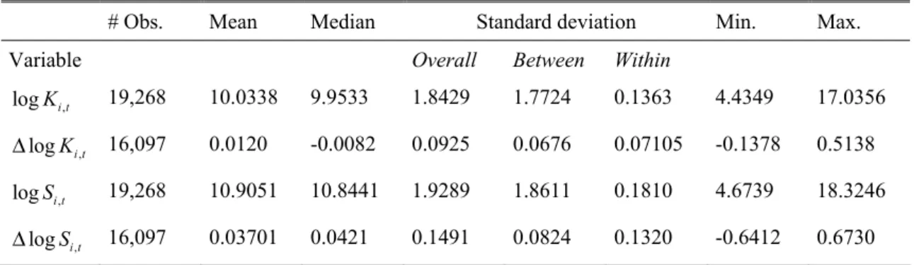
Table 1 gives the descriptive statistics for the continuous model variables: logK_{i t,} ,

,

logK_{i t}

Δ , logS_{i t,} , and ΔlogS_{i t,} , in the cleaned dataset of firms where at least three con-secutive firm-years are available. That many lags are needed to yield just one valid ob-servation in a first difference Arellano-Bond (1991) estimation of the adjustment equa-tion, if a uniform speed of adjustment is assumed and equation (4) can be written as a standard AR(1) with fixed effects. The breakdown of the standard deviation demon-strates that ample within-firm variation is present, as far as changes ΔlogK_{i t,} and

,

logS_{i t}

Δ are concerned.

Table 2 gives a breakdown of these same variables according to size classes. It shows the large number of small firms in the dataset: the two lesser size categories hold about the same number of firms than the two larger size classes, encompassing firms with 200 employees and more. Size, both in the table and in the estimations, is measured at the beginning of an uninterrupted string of observations in the cleaned sample, in order to exclude endogeneity in the classification. It has to be noted that the Ifo institute splits some of the very largest companies up into smaller sub-units if business activities,

in-vestment and markets can be analysed separately. These entities receive separate ques-tionnaires. Therefore, the distinction between small and large firms may at times be blurred: firm size measures the number of employees in an organisational entity that does not always coincide with a legal entity.12

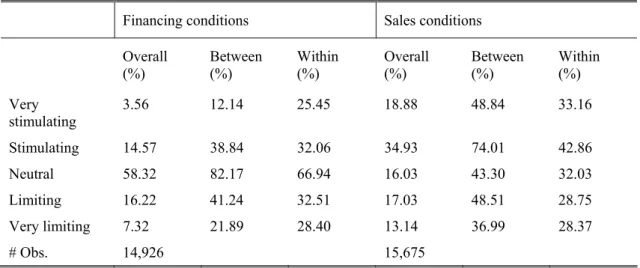
Table 3 gives an overview of the distribution for the financing conditions and the sales conditions variables generated by the question on factors for realised investment. It has been noted above that these two variables are underlying regime partition R(1) and the additional sales conditions indicator _{ωi t,} =ω'z_{i t,} , respectively. The number of observa-tions in Table 3 is smaller than in Table 1 for a variety of reasons. First, the question on investment factors was asked only from autumn 1989 on. Still, the capital stock and sales data from spring 1988 are kept in the data set in order to generate necessary lags and first differences. Furthermore, not every observation on sales and capital stocks from the spring survey can be matched to an observation of the preceding autumn sur-vey that yields the investment factors. Ultimately, about one tenth of respondents in the autumn survey do not give information on investment factors, as a response to this question is not required by the Ifo institute. In about half of these cases, no information on any factor is given. Often, this coincides with no investment being planned or having been undertaken. In the other 47% of cases were financing conditions information is missing, the sales indicator is present. This may be considered a source of selectivity, but it may also simply be due to the fact that not all firms are independent legal entities. Using the fact that Question 5 is asked for two consecutive years, I have imputed miss-ing data on investment factors from observations in adjacent years, wherever possible, in order to mitigate selectivity problems. Missing data in the autumn 1988 wave, where the question was not yet asked, were not imputed.

In Table 3, overall percentages summarise results in terms of firm-years. The distribu-tion of financing condidistribu-tions shows that "very stimulating" (3.6%) and "very limiting" (7.3%) episodes are relatively rare. In almost 60% of episodes, finance is considered "neutral". A share of 23.5% of firm-years are characterised by financing constraints, with financing conditions being "limiting" or "very limiting". The between columns repeat the breakdown in terms of observational units, giving the percentage of firms that ever had a specified value. Obviously, the percentages add up to more than 100, as many firms' responses vary over time. The within columns show this variation from a different perspective, giving the fraction of times firms report a certain value,

12 _{Due to confidentiality reasons, the units that are part of a larger conglomerate are not separately}

tional on that value being reported at last once. A time invariant categorical variable would be characterised by a value of 100% in each within entry.

As mentioned in the beginning, our estimator is specifically designed to make use of the within variation in regime information. Therefore Tables 4 and 5 give the transition matrices for the two regime partitions that may take three values, R(2) and R(3). Look-ing first at Table 4 featurLook-ing the three-level financLook-ing conditions indicator, we see that the regimes are moderately persistent: all three values are followed by the same value in more than 50% of cases. In both the first (stimulating or very stimulating) and the third (limiting or very limiting) categorise, also the off-diagonal elements are well filled, whereas the "neutral" category is followed by another value in only 20% of cases. A different picture results for the case of R(3) from Table 5. Whereas 72% of the uncon-strained expanders are unconuncon-strained expanders also in the next period, it is only 41% of the constrained expanders who find themselves in the same regime also in the next pe-riod. The rest defects with about the same probability to the first (unconstrained ex-panders) and the third regime (potential contractors). This clearly shows that a lot of noise would be introduced by fixing firm specific characteristics once and for all, not making use of within variation.

We now turn to Tables 6, 7 and 8 that hold the GMM estimations of the quasi-differ-enced adjustment equations. The tables all follow the same basic design. The first two columns hold the results for estimations that use the entire sample ("all firms"). In Col-umn (1), the target equation for the capital stock is given by equation (3) without further modifications. In Column (2), the target equation is augmented by dummies from the sales conditions indicator. Columns (3) and (4) hold the results for small firms, with 199 employees or less, again with and without augmenting the target equation by sales con-dition information. Finally, Columns (5) and (6) report the results for large firms, with 200 employees or more, again using two specifications for the target equation. The set of instruments is uniform over tables and was defined on the basis of prior specification search using an Arellano-Bond (1991) first difference estimator on a model with homo-geneous adjustment speed. I use lags 1-6 of regime dummies, lags 3-6 of logS_{i t,} and

,

logK_{i t} and time dummies. In addition, lags 2-6 of sales conditions dummies are used for the estimates with the enlarged target equation, Columns (2), (4) and (6) of each table.

Table 6 reports the results for Regime partition R(1) that derives directly from the fi-nancing factor for realised investment. The tables report the alpha values, which are equal to 1 minus the speed of adjustment. With one marginal exception in Column (1),

specifications tests do not reject the set of instruments. The Sargan-Hansen statistics of overidentifying restrictions are innocent and the LM(k) test on residual autocorrelation confirm that using as instruments the lags three and earlier of the capital stock and real sales variables is justified.

In all six columns, we see clearly that measured adjustment speed is decreasing when reported financing conditions get worse, although in some of the estimates there is an inversion for _α4 (finance limiting). In the regression without additional variables in the target equation, the measured adjustment speed in the estimations for the "all firms" sample differ as much as 0.3474 for the first regime (very stimulating) to 0.218 for the fifth regime (very limiting). The adjustment speeds for the set of estimates that include the sales condition information are somewhat lower and range between 0.268 for the first regime and 0.1874 for the fifth. This may be a result of the estimated target taking up more variation. Augmenting the target equation leads to more precise estimates of the adjustment coefficients in Table 6 and the other tables. In all estimates, the differ-ence between the first and the third regime (finance neutral) are especially marked. For each regime, measured adjustment speed is consistently higher for small firms, comparing adjustment speeds derived for the same specification of the target equation. In the third regime (finance neutral), adjustment speed is 0.2407 for small firms, 0.1777 for large firms and an intermediate 0.228 in the estimation that encompasses all firms. For the estimation using the sales indicator information in the target, the measured speeds are 0.2391 for small firms, 0.1666 for large firms and 0.1827 for the entire sam-ple. Equally important, we can see that financing conditions matter more for small firms. For them, the speeds of adjustment varies more between the extremes (0.3565 and 0.3469 if finance is very stimulating vs. 0.2644 and 0.2352 if finance is very limit-ing) than this is the case for larger firms (0.2074 and 0.1900 if finance is very stimulat-ing vs. 0.149 and 0.143 if finance is very limitstimulat-ing).

With five regimes, it is difficult to test for differences between individual regimes. In Table 7, I present results for the condensed regime partition R(2), where on each side the two extreme categories are aggregated. The general picture is similar. Again, the speed of adjustment is decreasing with financing conditions. However, there is barely any difference visible between the second category (finance neutral) and the third (fi-nance limiting or very limiting). This may be the result of the inversion for _α4 that was mentioned in the discussion of Table 6, as the categories four and five in R(1) are lumped together in R(2). Again, small firms show a clearly higher speed of adjustment in all regimes and for both basic specifications.

Testing coefficient restrictions shows that regime matters. The hypothesis _{α α1}= ₂ is rejected on a 5% level for both of the estimations that use all firms. For the subsets of small and large firms, the respective coefficient estimates do not differ significantly. For small firms, this may be due to the lower number of observations. In the case of large firms, the measured adjustment speeds do not differ much indeed.

In Table 8, the exercise is repeated using R(3) as regime partition. This regime partition closely corresponds to the underlying theoretic ideas and also takes a possible bias in the measurement of adjustment speeds for rapidly downsizing firms into account. I con-centrate on the comparison of the adjustment speed 1−_α1 for unrestricted stationary or expanding episodes with the adjustment speed 1−_α2 for financially constrained station-ary or expanding episodes. For estimates using the entire sample, the differences in ad-justment speed are significant on a 10% level for both specifications of the target equa-tion. Without additional variables in the target, it is 0.2599 for stationary or expanding unconstrained firms and 0.2047 for their constrained counterparts. Augmenting the tar-get equation by sales indicators leads to an adjustment speed of 0.2068 for stationary or expanding unconstrained firms and 0.1665 for their constrained counterparts. Repeating the differential analysis separately for small and for large firms shows that financing constraints do matter for small firms. Here, the adjustment speed is 0.3066 for uncon-strained firms vs. 0.2331 for conuncon-strained firms using the target equation without sales indicators and 0.2433 vs. 0.1658 with the augmented target equation. This latter result is strongly significant, with a p-value of 0.0140. For large firms, the measured differences are neither statistically nor economically significant: the adjustment speeds cluster around 0.18 for both specifications.

As a result from these estimations and tests, we see that financing constraints slow down the speed of adjustment of firms. Furthermore, this effect is concentrated or per-haps even limited to smaller firms. With large firms, no clear speed differential can be detected. Ultimately we see that the speed of adjustment of small firms is clearly higher than for large firms. These results fit extremely well to what was obtained by von Kalckreuth (2006) for capacity adjustment of UK firms, using an entirely different methodology on a different type of data.

6. Aggregate implications of adjustment heterogeneity

If the speed of adjustment is regime dependent, then the aggregate reaction to an overall shock depends on the composition, and changes in this composition are equivalent to changes in aggregate sensitivity. This is well known, but our method of relating the

dy-namic behaviour of individuals to survey information makes it particularly easy to trace the aggregate sensitivity and give up-to-date estimates about the current stance.

Graph 1 is based on the preferred regime partition R(3), with the results that were ob-tained using the entire sample. For demonstration purposes, I use the simple target equation specification, Table 8, Column (1), as it yields higher differences between re-gimes. The qualitative picture that results from using the results from the augmented target equation is very similar. The upper two panels of Graph 1 display the changing composition of the estimation panel with respect to adjustment regimes. The left panel refers to the unweighted averages, the right panel to the average weighted with the log of the real capital stock. It can easily be seen that the variation in composition is consid-erable and closely follows the business cycle in Germany.

The lower two panels show the aggregate sensitivity to a hypothetical aggregate shock that consists in an equiproportionate increase in the target level of all firms. Again both the unweighted and the weighted averages are given. The same type of approach would be possible for other, more complex adjustment equations, and various dynamic multi-pliers, eg first period, second, third etc. period effects. In the current setting, with one regime specific dynamic parameter, we simply need to multiply the shares with the as-sociated adjustment coefficient to get the one-period sensitivity of labour or capital de-mand with respect to an aggregate shock in the target in the last period. The time varia-tion in aggregate sensitivity is considerable, though not overwhelming: Aggregate sen-sitivity of capital demand is 0.247 in 1990, decreases to 0.215 in 1994 and returns to 0.250 in the last vintage of the micro data set, the year 1998.

The graph exemplifies how survey data on financing constraints or other regimes can be used for policy analysis. The aggregate sensitivity condenses the informational content of the microeconomic composition. With estimates of regime specific dynamics at hand, what drives the aggregate sensitivity is the changing composition of the aggregate. This composition is timely available in the course of the publication routines of survey agen-cies. When it comes to evaluating the survey data, the difficult process of estimating regime specific adjustment dynamics does not have to be repeated, as it is possible to rely on the coefficients estimated earlier.

References

Abel, Andrew B., and Janice C. Eberly, Optimal Investment with Costly Reversibility,

Review of Economic Studies Vol. 63 (1996), 581-593.

Abel, Andrew B., and Janice C. Eberly, Q Theory without Adjustment Costs and Cash Flow Effects without Financing Constraints, Unpublished manuscript, October 2001, revised October 2003.

Abel, Andrew B., Avinash Dixit, Janice C. Eberly and Robert S. Pindyck, Options, the Value of Capital and Investment, Quarterly Journal of Economics Vol. 111 (1996), 753-777.

Anderson, T.W., and Cheng Hsiao, Formulation and Estimation of Dynamic Models Using Panel Data, Journal of Econometrics Vol. 18 (1982), 47-82.

Arellano, Manuel, and Olympia Bover, Another Look at the Instrumental Variable Esti-mation of Error Component Models, Journal of Econometrics Vol. 68 (1995), 29-51.

Arellano, Manuel, and Stephen Bond, Some Tests of Specification for Panel Data: Monte Carlo Evidence and an Application to Employment Equations, Review of Economic Studies Vol. 58 (1991), 277-297.

Basu, Parantab, and Alexandra Guariglia, Liquidity Constraints and Firms' Investment Returns Behaviour, Economica Vol. 69 (2002), 563-81.

Bayer, Christian, Investment Dynamics with Fixed Adjustment Costs and Capital Mar-ket Imperfections, Journal of Monetary Economics Vol. 53 (2006), 1909-1947. Bean, Charles R., An Econometric Model of Manufacturing Investment in the UK, The

Economic Journal Vol. 91 (1981), 106-121.

Bentolila, Samuel and Guiseppe Bertola, Firing Costs and Labour Demand: How Bad is Eurosclerosis? Review of Economic Studies Vol. 57 (1990), 381-402.

Bernanke, Ben S., and Mark Gertler, Agency Costs, Net Worth, and Business Fluctua-tions, The American Economic Review Vol. 79 (1989), 14-31.

Bernanke, Ben S., and Mark Gertler, Inside the Black Box: The Credit Channel of Monetary Transmission, The Journal of Economic Perspectives Vol. 9 (1995), 27-48.

Bernanke, Ben S., Mark Gertler, and Simon Gilchrist, The Financial Accelerator and the Flight to Quality, The Review of Economics and Statistics Vol. 78 (1999), 1-15. Bernanke, Ben S., Mark Gertler, and Simon Gilchrist, The Financial Accelerator in a

Quantitative Business Cycle Framework, in Taylor, John B, and Michael Wood-ford (eds), Handbook of Macroeconomics Vol. 1 (Amsterdam, New York, etc.: North Holland, 1999), Ch. 21, 1341-1393.

Blundell, Richard, and Stephen Bond, Initial Conditions and Moment Restrictions in Dynamic Panel Data Models. Journal of Econometrics Vol. 87 (1998), 115-143.

Bond, Stephen, and Domenico Lombardi, To Buy or Not to Buy? Uncertainty, Irre-versibility and Heterogeneous Investment Dynamics in Italian Company Data.

IMF Staff Papers Vol. 53 (2007), 375-400.

Bond, Stephen, Julie Ann Elston, Jaques Mairesse and Benoît Mulkay, Financial Fac-tors and Investment in Belgium, France, Germany, and the United Kingdom: A Comparison Using Company Panel Data. The Review of Economics and Statistics

Vol. 85 (2003), 153-165.

Caballero, Ricardo J., and Eduardo M.R.A. Engel, Three Strikes and You're Out: Reply to Cooper and Willis, NBER Working Paper No. 10368 (2004).

Caballero, Ricardo J., Eduardo M.R.A. Engel and John C. Haltiwanger, Plant Level Adjustment and Aggregate Investment Dynamics, Brookings Papers on Economic Activity, 1995:2, 1-39.

Caballero, Ricardo J., Eduardo M.R.A. Engel and John C. Haltiwanger, Aggregate Em-ployment Dynamics: Building from Microeconomic Evidence, The American Economic Review Vol. 87 (1997), 115-137.

Chirinko, Robert S., and Ulf von Kalckreuth, Further Evidence on the Relationship be-tween Firm Investment and Financial Status, Discussion Paper 28/02, Economic Research Centre of the Deutsche Bundesbank, November 2002.

Cooper, Russell, and João Ejarque, Exhuming Q: Market Power vs. Capital Market Imperfections, NBER Working Paper No W8182, March 2001.

Cooper, Russell, and Jonathan L. Willis, A Comment on the Economics of Labor Ad-justment: Mind the Gap, American Economic Review Vol. 94 (2004), 1223-1237. Fazzari, Steven M., R. Glenn Hubbard, and Bruce C. Petersen, Investment-Cash Flow

Sensitivities are Useful: A Comment on Kaplan and Zingales, Quarterly Journal of Economics Vol. 115 (2000), 695-705.

Fazzari, Steven M., R., Glenn Hubbard, and Bruce C. Petersen, Financing Constraints and Corporate Investment, Brookings Papers on Economic Activity 1988:1, 141-195.

Gomes, João, Financing Investment, American Economic Review Vol. 91 (2001), 1263-1285.

Hansen, Lars, Large Sample Properties of Generalized Method of Moments Estimators,

Econometrica Vol. 50 (1982), 1029-1054.

Holtz-Eakin, Douglas, Whitney Newey, and Harvey S. Rosen, Estimating Vector Auto-regressions with Panel Data, Econometrica Vol. 56 (1988), 1371-1395.

Kaplan, Steven N., and Luigi Zingales, Do Investment-Cash Flow Sensitivities Provide Useful Measures of Financing Constraints? Quarterly Journal of Economics Vol. 112 (1997), 169-215.

Kaplan, Steven N., and Luigi Zingales, Investment-Cash Flow Sensitivities Are Not Valid Measures of Financing Constraints, Quarterly Journal of Economics Vol. 115 (2000), 707-712.

Sargan, John D., The Estimation of Economic Relationships Using Instrumental Vari-ables. Econometrica Vol. 26 (1958), 393-415.

von Kalckreuth, Ulf, Financial Constraints for Investors and the Speed of Adaptation: Are Innovators Special? Deutsche Bundesbank Discussion Paper Series 1: Eco-nomic Studies, No 20/2004.

von Kalckreuth, Ulf, Financial Constraints and Capacity Adjustment: Evidence from a Large Panel of Survey Data. Economica, Vol. 73 (2006), 691-724.

von Kalckreuth, Ulf (2008), Panel Estimation of State Dependent Adjustment When the Target Is Unobserved. Deutsche Bundesbank Discussion Paper Series 1: Eco-nomic Studies, No 09/2008.

Windmeijer, Frank, A Finite Sample Correction for the Variance of Linear Two-Step GMM Estimators”, Journal of Econometrics Vol. 126 (2005), 25-51.

Table 1: Descriptive statistics for continuous variables

# Obs. Mean Median Standard deviation Min. Max.

Variable Overall Between Within

, logKi t 19,268 10.0338 9.9533 1.8429 1.7724 0.1363 4.4349 17.0356 , logKi t Δ 16,097 0.0120 -0.0082 0.0925 0.0676 0.07105 -0.1378 0.5138 , logSi t 19,268 10.9051 10.8441 1.9289 1.8611 0.1810 4.6739 18.3246 , logSi t Δ 16,097 0.03701 0.0421 0.1491 0.0824 0.1320 -0.6412 0.6730

Notes: All values are in natural logarithms of multiples of 1.000 Deutsche Mark, 1991 prices. Values for net real capital stocks are generated using the eternal inventory method on the basis of panel information on fixed investment and real depreciation rates. Starting values are computed on the basis of reported number of employees and time specific sector capital-labour intensities computed from German national accounts data.

Table 2: Breakdown by firm size classes

Size classes # Firms logK _{i t,} ΔlogK_{i t,} logS i t, ΔlogSi t,

1-49 empl 619 7.5682 -0.0046 8.3284 0.0302

50-199 empl. 970 9.0500 0.0102 9.9118 0.0455

200 – 999 empl. 1,015 10.5367 0.0167 11.4293 0.0366

1000 and more empl. 567 12.4916 0.0199 13.4311 0.0313

All firms 3,171 10.0338 0.0120 10.9051 0.03701

Notes: See Table 1. Size classes are defined on the basis of employment information at the start of a con-secutive string of firm observations.

Table 3: Financing and sales conditions for realised investment: Tabulations and panel variation

Financing conditions Sales conditions

Overall

(%) Between (%) Within (%) Overall (%) Between (%) Within (%)

Very stimulating 3.56 12.14 25.45 18.88 48.84 33.16 Stimulating 14.57 38.84 32.06 34.93 74.01 42.86 Neutral 58.32 82.17 66.94 16.03 43.30 32.03 Limiting 16.22 41.24 32.51 17.03 48.51 28.75 Very limiting 7.32 21.89 28.40 13.14 36.99 28.37 # Obs. 14,926 15,675

Notes: Tabulations are for factors relating to investment carried out in the current year, given in percent-age terms. See the text for the exact wording of the survey question. Overall percentpercent-ages summarise re-sults in terms of firm-years. Between columns repeats the breakdown in terms of firms, giving the per-centage of firms that ever reported a specified value. Within columns give the fraction of time firms report a certain value, conditional on that value being reported at least once. A time invariant categorical vari-able would have a tabulation with each entry equal to 100% in the within column

Table 4: Transition matrix for regime partition R(2)

Stimulating or

very stimulating Neutral Limiting very limiting or Total

Stimulating or very stimulating 1,092 (54.09%) 597 (29.57%) 330 (16.34%) 2,019 (100.0%) Neutral 627 (9.14%) 5,418 (78.99%) 814 (11.87%) 6,859 (100.0%) Limiting or very limiting 355 (12.54%) 744 (26.28%) 1,732 (61.18%) 2,831 (100.0%) Total 2,074 (17.71%) 6,759 (57.72%) 2,876 (24.56%) 11,709 (100.0%)

Notes: Tabulations are for factors relating to investment carried out (or planned) for the current year, given in percentage terms. See the text for the exact wording of the survey question. The outcomes of financial factors for realised investment are condensed to three values by aggregating "very stimulating" and "stimulating" to one category and "very limiting" and "limiting" to another.

Table 5: Transition matrix for regime partition R(3) Finance not

limit-ing and stationary or expanding Finance limiting, and stationary or expanding Potentially down-sizing Total Finance not limiting and stationary or expanding 3,462 (71.96%) 448 (9.31%) 901 (18.73%) 4,811 (100.0%) Finance limiting, and stationary or expanding 364 (29.76%) 503 (41.13%) 356 (11.87%) 1,223 (100.0%) Potentially downsizing 905 (12.54%) 199 (26.28%) 1,437 (61.18%) 2,541 (100.0%) Total 4,731 (55.17%) 1,150 (13.41%) 2,694 (31.42%) 8,575 (100.0%)

Notes: Regime partition R(3) is generated using responses on expected factors for next period's invest-ment, lagged once, see the description in the main text. The first category combines the levels "very stimulating,", "stimulating" and "neutral" of the financing conditions indicator with the levels "very stimulating", "stimulating" and "neutral" of the sales conditions indicator. The second category combines the same levels of the sales indicator with the levels "limiting" or "very limiting" of the financing condi-tions indicator. The third category collects all observacondi-tions where sales condicondi-tions were described as "limiting" or "very limiting".

Table 6: Adjustment speed according to financing conditions

Regime partition R(1), 5 regimes, based on factors for realised investment Dependent variable: , logK_{i t} Δ All firms(1) w/o sales cond. ind. in target (2) All firms with sales cond. ind. in target (3) SMEs w/o sales cond. ind. in target (4) SMEs with sales cond. ind. in target. (5) Large w/o sales cond. ind. in target (6) Large with sales cond. ind. in target Regime specific adjustment coeff. 1 α (fin. very stimulating) 0.6526 (0.0788) 0.7319 (0.0593) 0.6435 (0.1043) 0.6531 (0.0832) 0.7926 (0.0540) 0.8100 (0.0482) 2 α (finance stimulating) 0.7194 (0.0343) 0.7798 (0.0308) 0.6898 (0.0547) 0.7149 (0.0451) 0.8106 (0.0332) 0.8187 (0.0296) 3 α (finance neutral) 0.7720 (0.0286) 0.8173 (0.0231) 0.7593 (0.0381) 0.7609 (0.0374) 0.8223 (0.0294) 0.8334 (0.0229) 4 α (finance limiting) 0.7540 (0.0351) 0.7998 (0.0295) 0.7246 (0.0462) 0.7500 (0.0516) 0.8233 (0.0328) 0.8385 (0.0263) 5 α

(fin. very limiting)

0.7802

(0.0349) 0.8126 (0.0311) 0.7356 (0.0578) 0.7648 (0.0587) 0.8510 (0.0348) 0.8507 (0.0309)

Additional vars. in target equation:

Time dummies yes yes yes yes yes yes

Sales conditions

indicator dummies no yes no yes no yes

Observations and specification tests Sargan-Hansen test 2_{(203) 239.5} 0.040 p χ = = 2_{(319) 331.6} 0.302 p χ = = 2_{(203) 216.2} 0.250 p χ = = 2_{(319) 321.4} 0.452 p χ = = 2_{(203) 218.6} 0.215 p χ = = 2_{(319) 307.8} 0.663 p χ = = LM (1) test, p-value 0.000 0.000 0.000 0.000 0.000 0.000 LM (2) test, p-value 0.000 0.000 0.029 0.033 0.000 0.000 LM (3) test, p-value 0.355 0.531 0.944 0.979 0.054 0.055 # Firms 2,753 2,744 1,299 1,292 1,454 1,452 # Obs. 10,723 10,675 4,426 4,398 6,297 6,277

Notes: Estimates for regime specific adjustment of the real capital stock as given in equation (4). Esti-mation method: GMM on the basis of Quasi-Difference transforEsti-mation QD2 as described in von Kalckreuth (2008) and this text. For each estimate, the target equation for the capital stock contains

, 1 ,

logK_{i t−} −logS_{i t}, time dummies and a firm fixed effect, modelling a reversion of capital intensity to a

firm specific value conditioned by time effects to capture macroeconomic effects and technical progress. In estimates (2), (4) and (6), the target equation also contains category dummies for the sales conditions factor. Regime partition is based on the financing conditions indicator relating to investment carried out in the current year as stated by respondents, with each regime corresponding to one value the indicator may take, cf. Table 3. See the main text for the exact wording of the survey question. Instruments: lags

1-6 of regime dummies, lags 3-1-6 of logS_{i t,} and logK_{i t,} and time dummies, in estimates (2), (4) and (6)

additionally lags 2-6 of sales conditions dummies. The Sargan-Hansen statistic is a test of overidentifying restrictions proposed by Sargan (1958) and Hansen (1982). The LM(k) tests are the p-values for the La-grange Multiplier statistics for serial correlation of order k proposed by Arellano and Bond (1991). The robust standard errors from the second step estimation with a small sample correction based on Wind-meijer (2005) are in parentheses. Estimation was executed using DPD package version 1.2 on Ox version 3.30 and extensive user written Ox routines.