Global Liquidity Risk in the Foreign Exchange
Market
Chiara Banti, Kate Phylaktis, and Lucio Sarno
yAbstract
Using a broad data set of 20 US dollar exchange rates and order ‡ow of institutional
investors over 14 years, we construct a measure of liquidity in the foreign exchange (FX)
market. Our global FX liquidity measure is the analogue of the well-known
Pastor-Stambaugh liquidity measure for the US stock market. We show that this measure has
reasonable properties, and that there is a strong common component in liquidity across
currencies. Finally, we provide evidence that liquidity risk is priced in the cross-section
of currency returns, and estimate the liquidity risk premium in the FX market around
4.7% per annum.
Keywords: foreign exchange; liquidity; order ‡ow; microstructure.
JEL Classi…cation: F31; F37; G12; G15.
Financial support is gratefully acknowledged from the Economic and Social Research Council.
yBanti, Chiara.Banti.1@cass.city.ac.uk, Cass Business School, City University, 106 Bunhill Row, London,
EC1Y 8TZ, UK; Phylaktis, K.Phylaktis@city.ac.uk, Cass Business School, City University, 106 Bunhill Row, London, EC1Y 8TZ, UK, +44 (0)20 7040 8735; and Sarno, Lucio.Sarno@city.ac.uk, Cass Business School, City University, 106 Bunhill Row, London, EC1Y 8TZ, UK, +44 (0) 20 7040 8772, and Centre for Economic Policy Research (CEPR).
I
INTRODUCTION
The foreign exchange (FX) market is considered to be highly liquid. In terms of turnover, the average daily market activity in April 2010 was $3.98 trillion (BIS (2010)). However, there are large di¤erences across currencies: 66% of the FX market average daily turnover in April 2010 involves the six most traded pairs of currencies. In addition to the di¤erent liquidity levels across currencies, liquidity changes over time. Analyzing bid-ask spread determinants, Bessembinder (1994), Bollerslev and Melvin (1994), and Lee (1994) document signi…cant time-variation of the bid-ask spreads in FX market. Focusing on intra-daily data, Hsieh and Kleidon (1996) present a high variation in spreads and trading volume in di¤erent FX markets.
Using a unique data set comprising daily order ‡ow data for 20 exchange rates spanning 14 years, we build a measure of liquidity based on the Pastor and Stambaugh (2003) measure, which was originally developed for the US stock market. Analyzing the properties of the individual currency liquidity measures, we …nd that they are highly correlated, suggesting the presence of a common component across them. The presence of a common component is consistent with the notion that liquidity is largely driven by shocks that a¤ect the FX market as a whole rather than individual currencies. We then construct a measure of innovations in global FX liquidity (unexpected liquidity) and show that it explains a sizeable share of liquidity innovations in individual currencies.
In the stock market literature, several papers …nd signi…cant co-movement of liquidity cross-sectionally (Datar, Naif, and Radcli¤e (1998), Huberman and Halka (2001), Chordia, Roll, and Subrahmanyam (2000, 2001), Hasbrouck and Seppi (2001), Lesmond (2005)). In contrast, the FX market has received much less attention. The presence of such co-movement in the FX market during the recent crisis period is documented in Melvin and Taylor (2009)
and Mancini, Ranaldo, and Wrampelmeyer (2011). However, to our knowledge, this is the …rst paper to study global FX liquidity covering a long sample period which includes both crisis and non-crisis periods drawing on the behavior of both developed and emerging market currencies, where liquidity is more of an issue.
Next, taking the perspective of a US investor, we ask whether unexpected changes (inno-vations) in FX market liquidity a¤ect exchange rate movements. In other words, we examine whether there is a systematic liquidity risk premium in the FX market. Adopting di¤erent proxies for liquidity, some studies …nd a relationship between changes in liquidity and expected stock returns, detecting a liquidity risk premium in the stock market (Pastor and Stambaugh (2003), Acharya and Pederson (2005), Chen (2005), Korajczyk and Sadka (2008), Hasbrouck (2009), Lee (2011)). Estimating systematic liquidity risk as the covariance of exchange rate returns and innovations in common liquidity, we identify a liquidity risk premium by em-ploying standard empirical asset pricing tests and the portfolio construction techniques …rst applied to FX data by Lustig and Verdelhan (2007). These methods allow us to eliminate currency-speci…c sources of returns by taking into account the common component of the excess returns related to systematic liquidity risk. Our empirical asset pricing results are sup-portive of the presence of a risk premium associated with FX market liquidity. The market price of liquidity risk stays signi…cant even after conditioning on other common risk factors in FX asset pricing analysis, such as the dollar and carry risk factors. Moreover, our results are robust to a number of tests including volume-related weighting of currencies to calculate the common liquidity measure, di¤erent rebalancing horizons, and an alternative estimation method.
Furthermore, our broad data set containing 10 emerging market currencies allows us to study their particular behavior. We …nd that the sensitivities of emerging market
curren-cies returns to innovations in market liquidity are less variable and exhibit a lower portfolio turnover than those of developed country currencies. Moreover, the liquidity risk premium associated with emerging market currencies is signi…cantly higher than that of the whole data set. Thus, while signi…cant for the cross-section of the whole data set, global liquidity risk is especially important for emerging market currencies.
The paper is organized as follows. Section 2 provides an overview of the relevant literature. In Section 3 we describe the data set and provide some descriptive statistics. The methodology for the construction of the liquidity measure, the estimation of the innovation in common liquidity, the investigation of the presence of a systematic liquidity risk premium, and the empirical asset pricing exercise are described in Section 4. The empirical results are reported in Section 5, where we document the presence of a common component in liquidity across currencies, we identify a liquidity risk premium, and we estimate its market price. Section 6 contains some further analysis, including an extension of the liquidity risk de…nition, an analysis of liquidity risk employing two alternative liquidity estimations, an investigation on currencies of emerging markets and less traded developed countries and the liquidity risk premium associated to them, and an additional study focusing on liquidity risk in the recent …nancial crisis following the Lehman Brothers collapse in September 2008. We report some robustness checks in Section 7. Finally, Section 8 concludes.
II
LITERATURE REVIEW
A
Liquidity and the FX market
In the FX market, dealers provide liquidity to the market and quote a price after receiving orders from customers and other dealers. With the increase in data availability, a literature
analyzing the price impact of order ‡ow has emerged in the last decade, documenting that order ‡ow can successfully explain a sizable share of the movements in the exchange rates (Evans and Lyons (2002a)).1
Due to the heterogeneity of market participants, the FX market is characterized by infor-mational asymmetries, so that dealers gather disperse information from the orders placed by their customers (e.g. Lyons (1997)). Indeed, FX market practitioners’surveys highlight how order ‡ow is seen as a preferred channel for dealers to obtain private and dispersed information from customers (Goodhart (1988), Cheung and Chinn (2001), Gehrig and Menkho¤ (2004)). In this sense, the information channel works from the dealer’s own customer order ‡ow and from the aggregate market customer order ‡ow which can be inferred from the interdealer and brokered trading. As a consequence, the presence of asymmetric information in the market in‡uences liquidity (Copeland and Galai (1983), Kyle (1985), Glosten and Milgrom (1985), Admati and P‡eiderer (1988)). Dealers quote a price by balancing the expected total revenues from liquidity trading against the expected total losses from informed trading. Copeland and Galai (1983) suggest that liquidity decreases with greater price volatility in the asset being traded, with a higher asset price level, and with lower volume. In this respect, Bollerslev and Melvin (1994) …nd a signi…cant negative relationship between the bid-ask spread and exchange
1Order ‡ow re‡ects buying pressure for a currency and it is typically calculated as the sum of signed trades.
The sign of a given transaction is assigned with respect to the aggressive party that initiates the trade. Evans and Lyons (2002a) provided the seminal evidence in this literature, showing how order ‡ow is a signi…cant determinant of two major bilateral exchange rates, and obtaining coe¢ cients of determination substantially larger than the ones usually found using standard structural models of nominal exchange rates. Their results are found to be fairly robust by subsequent literature (e.g. Payne (2003), Bjønnes and Rime (2005), Killeen, Lyons and Moore (2006)). Moreover, Evans and Lyons (2005a, 2006) argue that gradual learning in the FX market can generate not only explanatory, but also forecasting power in order ‡ow, as documented, for example, in Rime, Sarno and Sojli (2010).
rate volatility in the interbank market trading of the DM/USD.
Analyzing the intra-daily trading of DM/USD in two interbank FX markets (London and New York), Hsieh and Kleidon (1996) …nd that the volatility patterns in spreads and trading volume are not consistent with standard asymmetric information models. So, the observed shifts in transaction costs and trading volume (which can be viewed as proxies for liquidity) are not related to information ‡ows. They suggest that the high volatility of these measures could be explained by the inventory consideration of dealers. In her empirical analysis, Bessembinder (1994) …nds that bid-ask spreads of a set of currency pairs (USD against GBP, CHF, JPY and DM for 14 years from 1979 until 1992) widen with forecasts of inventory price risk and with a measure of liquidity costs. In addition, they identify a seasonal pattern in changes in spreads: spreads widens before weekends and nontrading intervals. They relate these observed patterns to inventory control conditions. A dealer with a larger currency inventory than desired will set a lower price to attract buyers, known as ‘quote shading’. According to the theoretical model by Amihud and Mendelson (1980), the market maker’s constraints on his short and long stock inventory positions in‡uence the level of liquidity of the market. Furthermore, liquidity will depend upon the factors that in‡uence the risk of holding inventory (Stoll (1978), Ho and Stoll (1981)). According to Grossman and Miller (1988), the provision of liquidity depends on the cost incurred by the market maker to maintain its presence in the market. This cost is inversely related to the number of market makers which are operating in the market. As a result, the larger the number of market makers in the market, the lower is the cost for immediacy and the more liquid is the market, in terms of lower price impact of trades. Focusing on the liquidity provided by the traders in the market, Brunnermeier and Pedersen (2009) extend the Grossman and Miller’s model to include the interaction of funding liquidity with the provision of liquidity by speculators. Under certain conditions, this interaction leads
the market to a liquidity spiral: speculators’liquidity constraints reduce market liquidity that will further tighten the constraints.
In his empirical analysis of a dealer’s trading activity in the DM/USD market, Lyons (1995) …nds positive evidence of the e¤ects of both the inventory control and the informational asymmetry channels. Speci…cally, running a regression of the changes in exchange rate on the incoming orders, the dealer’s inventory at the beginning of the period and other variables, Lyons (1995) reports positive and signi…cant coe¢ cients associated with the two variables of interest, transaction orders and inventory at the beginning of the period. On the other hand, Bjønnes and Rime (2005) document a strong information e¤ect on the trading activity of four dealers from a large Scandinavian bank. They …nd these results both taking into account the size of the orders and considering the direction of trades.
B
Measures of liquidity
The bid-ask spread is the most widely used measure of liquidity in the literature. In this respect, Stoll (1989) determines the relative importance of each of the three components of the spread (order processing costs, inventory control cost and adverse selection costs) from the covariance of transaction returns. In the FX market, much research has been carried out on the bid-ask spread e.g. see Bessembinder (1994), Bollerslev and Melvin (1994), Lee (1994), and Hsieh and Kleidon (1996). However, Grossman and Miller (1988) highlight a key limitation of the bid-ask spread as a measure for liquidity: this method gives the cost of providing immediacy of the market maker in the case of a contemporaneous presence of buy and sell transactions. In reality, this is almost never the case, also considering that the presence of the market maker is justi…ed by the need to provide immediacy to the transaction needs of the customers.
Apart from measures related to the transaction cost, other measures were developed to proxy the price impact of transactions. Pastor and Stambaugh (2003) propose a liquidity cost method that measures the temporary price change, in terms of expected reversal, due to signed transaction volume. This measure is based on the intuition that lower liquidity is accompanied by a higher volume-related return reversal. Another measure of this kind is the market depth measure of Kyle (1985)’s model. Market illiquidity is estimated as the impact of transactions on an asset prices. The intuition behind this measure is: the more liquid a market, the lower the impact of the transactions on prices. Furthermore, Amihud (2002)’s illiquidity ratio measures the elasticity of liquidity. This is calculated as the daily measure of absolute stock returns to its dollar volume, averaged over some period.
These liquidity measures have been developed and tested mainly for the stock market (e.g. see Naes, Skjeltorp, and Ødegaard (2010)). In fact, their application to the FX market can be quite problematic due to its speci…c characteristics and the di¢ culty of gathering order ‡ow and volume data. As a result, liquidity in the FX market has been investigated in only a few papers.
Evans and Lyons (2002b) address the issue of time-varying liquidity in the FX market using the price impact of order ‡ow as a proxy for liquidity. More recently, Mancini, Ranaldo, and Wrampelmeyer (2011) apply a modi…ed version of Pastor and Stambaugh’s measure to the FX market by building a daily measure of liquidity for about one year of order ‡ow data during the recent …nancial crisis. In our paper, we also apply the Pastor and Stambaugh’s measure of liquidity but we are able to rely on 14 years of order ‡ow data and 20 exchange rates.
C
Liquidity risk premium
Starting from the seminal paper by Amihud and Mendelson (1986), several papers model and empirically test the relationship between liquidity and expected stock returns (Brennan and Subramahmanyan (1996), Brennan, Chordia, and Subrahmanyam (1998), Datar, Naif, and Radcli¤e (1998)). A higher return is demanded by traders when stock liquidity is lower and transaction costs are higher. Most of the papers study the US stock market, but the same result is documented by Bekaert, Harvey, and Lundblad (2007) for emerging markets. The same result holds true for other assets: Amihud and Mendelson (1991), among others, …nd a signi…cant spread in the yields of Treasury notes and bills due to a liquidity risk premium.
Having investigated the e¤ect of the level of liquidity on expected equity returns, some studies also focus on the time variation of liquidity and on its co-movements cross-sectionally. Chordia, Roll, and Subrahmanyam (2000) analyze the correlated movements of liquidity both at industry and at market level. After controlling for determinants of liquidity such as volatil-ity, prices and volume, they document signi…cant common innovations in liquidity in the stock market. Similar conclusions are reached also by other authors. Huberman and Halka (2001) …nd that there is a systematic and time-varying component in stock market liquidity. A less clear-cut conclusion is reached by Hasbrouck and Seppi (2001), who …nd evidence of weak co-movement in stock market liquidity measures constructed from intra-daily data. Employing a longer data set of intra-daily stock market data, Chordia, Roll, and Subrahmanyam (2001) con…rm the presence of a common component in stock market liquidity, and then present an investigation of the possible determinants of the observed variation in market liquidity and trading activity over time. The determinants they consider are inventory control variables (such as daily returns and volatility) and informed trading variables (such as dummies for macroeconomic announcement dates).
Finally, some studies examine the implications of the documented time-variation in com-mon liquidity for asset returns, controlling for the presence of a priced liquidity risk in stock returns. In their analysis, Pastor and Stambaugh (2003) …nd that the sensitivities of stock returns to common liquidity innovations are priced. Acharya and Pederson (2005) broaden the analysis of a security’s liquidity risk to include the commonality in the liquidity risk and the covariance of individual assets’ liquidity with the market return, as well as Pastor and Stambaugh’s liquidity measure. By doing so, they develop a liquidity-adjusted Capital Asset Pricing Model (CAPM) and …nd empirical support for the presence of a priced liquidity risk. De…ning the common liquidity risk proxy as the common component of di¤erent liquidity measures, Chen (2005) and Korajczyk and Sadka (2008) …nd evidence that systematic liq-uidity risk is priced. Employing a di¤erent proxy for liqliq-uidity, Hasbrouck (2009) also …nds a positive relation between liquidity and stock returns, but reports two problematic issues: the relationship is a¤ected by seasonality and the coe¢ cients are too large to be explained only by the changes in traders’compensation for providing liquidity. In an empirical application of Acharya and Pedersen’s (2005) liquidity-adjusted CAPM, Lee (2011) identi…es a systematic global liquidity risk premium in stock returns. In particular, he …nds a premium related both to the commonality in liquidity and the covariance of individual stocks’liquidity and the stock market return.
III
DATA
A
Description of the data
The data set analyzed in this paper comprises daily data of 20 exchange rates and their order ‡ow for a time period of 14 years, from April 14, 1994 to July 17, 2008. Its uniqueness is the
wide cross section of currencies available for a long time period, including a signi…cant number of emerging markets. Of the 20 currencies in our data seta, 10 are of developed economies (Australian dollar, Canadian dollar, Danish krone, euro, Great Britain pound, Japanese yen, New Zealand dollar, Norwegian kroner, Swedish krona, and Swiss franc) and 10 are of emerging markets (Brazilian real, Chilean peso, Czech koruna, Hungarian forint, Korean won, Mexican peso, Polish zloty, Singapore dollar, South African rand, and Turkish lira). The abbreviations for these currencies used in the paper are given in Appendix A.
Log returns are calculated from the FX spot exchange rates of the US dollar versus the currencies and are obtained from Datastream. They are the WM/Reuters Closing Spot Rates. These rates are provided by Reuters at around 16 GMT.
Log-exchange rate returns are calculated as:
(1) rt = ln(St) ln(St 1)
where St is the FX spot rate of the US dollar versus the currency.
In order to calculate FX excess returns, one month forward exchange rates are obtained from Datastream and provided by WM/Reuters. Excess returns are calculated as follows:
(2) ert= ln(St+1) ln(Ft)
where Ft is the one-month forward exchange rate.
Turning to order ‡ow, the FX transaction data is obtained from State Street Corpora-tion (SSC). As one of the world’s largest custodian instituCorpora-tions, SSC counts nearly 10,000 institutional investor clients with 11.9 trillion US dollar under custody. They record all the transactions in these portfolios, including FX operations. The data provided by SSC is the
daily order ‡ow aggregated per currency traded. Order ‡ow data is de…ned as the overall buying pressure on the currency and is expressed in millions of transactions (number of buys minus number of sells in a currency).
The sample period is generally from April 14, 1994 to July 17, 2008. For a group of currencies the sample for the liquidity analysis is shorter due to limited data availability from the providers. The sample period for the CZK starts on December 12, 1994 due to limited data availability of the spot exchange rate on the USD from Datastream. Also the sample period starts at a later date for these currencies due to limited data availability from SSC: CLP starts on October 4, 1995, HUF starts on September 30, 1994, and PLN starts on August 22, 1995. In addition, the BRL observations are considered from January 15, 1999, when the real was introduced as national currency and de…ned as independently ‡oating, and the observations for the EUR start on December 31, 1998. Furthermore, for the portfolio analysis and the following asset pricing exercise the sample period is shorter for BRL (from March 29, 2004), HUF (from October 27, 1997), KRW (from February 11, 2002), and PLN (from February 11, 2002) due to limited data availability of the one-month forward exchange rate on the USD from Datastream.
B
Descriptive statistics
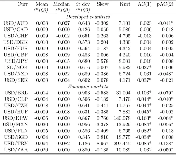
Table 1 presents some descriptive statistics of the log returns, grouped in developed and emerging countries. In general, emerging markets’currencies present a higher standard devi-ation than developed countries’currencies. Furthermore, log returns of developed currencies present low …rst and second order autocorrelation. In contrast, most of the emerging mar-ket currencies exhibit positive signi…cant …rst-order autocorrelation and negative signi…cant second-order autocorrelation.
Insert Table 1 here
-Table 2 shows some descriptive statistics for the order ‡ow data. On average, the largest positive order ‡ow during the sample for developed countries is for AUD and CAD, con…rming the anecdotal evidence of strong net demand for commodity currencies during this sample period, whereas the lowest is for DKK. In emerging markets, the largest average order ‡ow is for CLP, and the lowest for BRL. The order ‡ow for emerging markets generally presents a higher standard deviation than for developed countries. Furthermore, the order ‡ow data exhibit strong autocorrelation for all currencies in the sample, ranging from 76% for AUD up to 89% for TRY. For most of the emerging markets, the second-order autocorrelation is also signi…cant.
In the last column we report the correlation between the order ‡ow and the log return of the US dollar versus the currency. The correlation is signi…cant for most of the currencies. It is higher for the currencies of the advanced economies in the sample. All the correlations are positive, as expected. A positive order ‡ow indicates buying pressure for the currency, which causes the currency to appreciate. The results of the correlation analysis are comparable to the ones reported by Froot and Ramadorai (2005), who use a similar data set from the same source over a shorter sample.2
Insert Table 2 here
-2However, note that order ‡ow in Froot and Ramadorai (2005) is measured in millions of dollars, whereas
our order ‡ow series is de…ned as in the majority of papers since Evans and Lyons (2002a), in terms of net number of transactions. Nevertheless, the descriptive statistics suggest that the properties of the data are qualitatively the same.
IV
METHODOLOGY
A
Construction of the liquidity measure
Starting from Evans and Lyons (2002a), several papers document a signi…cant price impact of order ‡ow in the FX market.
Running the simple Evans and Lyons regression of log returns on contemporaneous order ‡ow:3
(3) ri;t = i+ i xi;t +"i;t;
we expect to …nd a positive coe¢ cient associated with the contemporaneous order ‡ow x. A positive order ‡ow causes the currency to appreciate, which leads to an increase in the exchange rate quoted as US dollar versus the foreign currency.
Following Pastor and Stambaugh (2003), we measure liquidity as the expected return re-versal accompanying order ‡ow. Pastor and Stambaugh’s measure is based on the theoretical insights of Campbell, Grossman, and Wang (1993). Extending the literature relating time-varying stock returns to non-informational trading (e.g. De Long, Shleifer, Summers, and Waldmann (1990)), Campbell, Grossman, and Wang develop a model relating the serial cor-relation in stock returns to trading volume. A change in the stock price can be caused by a shift in the risk-aversion of non-informed (or liquidity) traders or by bad news about future cash ‡ow. While the former case will be accompanied by an increase in trading volume, the
3As reported in the data description section, the order ‡ow is related to all the transactions in a speci…c
currency, irrespective of the currency against which the transaction takes place. However, in the regression analysis, we consider the exchange rate of the US dollar versus the currency, assuming the US dollar to be the major currency against which the transactions are made.
latter will be characterized by low volume. In fact, risk-averse market makers will require an increase in returns to accommodate liquidity traders’ orders. The serial correlation in stock returns should be directly related to the trading volume. The Pastor and Stambaugh’s measure captures this relationship and builds a proxy for liquidity given this return reversal due to the behavior of risk-averse market makers. While they use signed trading volume as a proxy for order ‡ow, we employ directly order ‡ow.
To estimate the return reversal associated with order ‡ow, we extend regression (3) above to include lagged order ‡ow:
(4) ri;t = i+ i xi;t+ i xi;t 1+"i;t:
We estimate this regression using daily data for every month in the sample, and then take the estimated coe¢ cient for to be our proxy for liquidity. Our monthly proxy for liquidity of a speci…c exchange rate is:
(5) Li;m =bi;m;
where the subscriptm refers to the monthly frequency of the series. If the e¤ect of the lagged order ‡ow on the returns is indeed due to illiquidity, ishould be negative and reverse a portion of the impact of the contemporaneous ‡ow, since iis expected to be positive. In other words, contemporaneous order ‡ow induces a contemporaneous appreciation of the currency in net demand ( i >0), whereas lagged order ‡ow partly reverses that appreciation ( i <0).
Other methodologies have been used in the literature to empirically estimate liquidity within regression analysis. In particular, in Evans and Lyons (2002b) the contemporaneous
impact, changed of sign, corresponds to the measure of market depth from Kyle (1985)’s model. Of the possible speci…cations, Pastor and Stambaugh (2003) estimate liquidity from a regression of returns on lagged order ‡ow including lagged returns to account for serial correlation. We specify our regression not including the lagged returns because our order ‡ow are estimated with error and thus the inclusion of lagged returns could result in an under-estimation of liquidity. However, further in the paper, we will analyze these other methodologies and we will discuss them in more detail.
B
Estimation of a common liquidity measure
Subsequently, we construct a measure of common liquidity (DLm) by averaging across cur-rencies the individual monthly liquidity measures (e.g. Chordia, Roll, and Subrahmanyam (2000), Pastor and Stambaugh (2003)), excluding the two most extreme observations:
DLi;m = (Li;m Li;m 1) (6) DLm = 1 N N X i=1 DLi;m: (7)
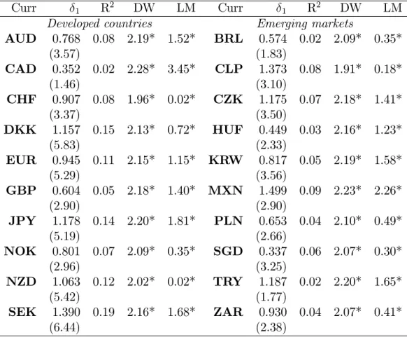
In order to account for potential autocorrelation of some of the individual liquidity series and isolate liquidity innovations, the unexpected component of common liquidity (DLCm) is obtained as the residual of an AR(1) model of the common liquidity measure.4 In other words,
we estimate:
(8) DLm = 0+ 1DLm 1+"t
4An AR(1) model is enough to eliminate serial correlation in the residuals. Also note that we use the term
and set DLC
m =b"m.
Following Chordia, Roll, and Subrahmanyam (2000), we then regress the individual liquid-ity measures (DLi;m) on the measure of unexpected common liquidity risk (DLCm) to further investigate the commonality in the liquidity innovations across currencies:
(9) DLi;m= 0i+ 1iDLCm+ i;t:
In our further analysis, we will build an alternative measure of common liquidity as a volume-weighted average of the individual liquidity measures.
C
Analysis of systematic liquidity risk
Next, we investigate whether common liquidity risk is priced in FX returns. In order to do so, we construct four portfolios for each year based on the ranking of the historical sensitivities of currencies’returns to common liquidity risk.5 Linking the return of each of the four portfolios year after year, the returns of the portfolios are then compared, and we expect the portfolios more sensitive to liquidity risk to have a higher excess return than the less sensitive portfolios. The analysis starts from January 1997 to account for the start date of the forward rate data from Datastream and it is conducted at every year-end. For each currency, the liquidity measure is estimated by the coe¢ cient associated with the lagged order ‡ow from regression (4), run with the past observations available at each year-end starting from January 1999, to allow for at least two years of past data for the estimations. At each year-end, the monthly series of common liquidity for the past available period is also calculated according to equations
5In other words, we estimate the sensitivity to unexpected common liquidity for each exchange rate using
non-overlapping years, and this gives us an estimate of the sensitivity per year for each exchange rate. Then, we sort currencies on the basis of the estimated sensitivities into four portfolios, which are rebalanced yearly.
(6) to (8).
Then, the sensitivity of each currency’s return to the common liquidity innovation is esti-mated with a regression of the monthly returns on the common liquidity measure estiesti-mated at each year end:
(10) ri;m= 0i+ 1iDL
C
m+"i;m:
At this point, the currencies are sorted according to the estimated parameter 1, which captures the sensitivity to common liquidity. Based on this ranking, four portfolios are con-structed with …ve equally-weighted currencies at each year-end: the …rst portfolio containing the least sensitive currencies to liquidity risk and the fourth being made of the most sensitive ones. The return of each portfolio for the following year is then calculated from the returns of each of the …ve equally-weighted currencies. For each portfolio a return series is obtained by linking the return calculated in each year. Having constructed the portfolios based on their sensitivity to our liquidity measure, we expect the most sensitive portfolio to be associated with a higher return in compensation for the higher liquidity risk associated with it.
D
Empirical asset pricing
Following the comparison of the liquidity-sorted portfolios’ excess returns, we proceed to investigate whether systematic liquidity risk is priced in the cross-section of excess returns of the portfolios.
In order to establish whether systematic liquidity risk is priced, we conduct a Fama-MacBeth (1973) analysis starting from January 1999. Taking the perspective of a US investor, we test whether a liquidity risk factor prices the excess returns of the portfolios sorted accord-ing to the sensitivities of the currencies’return to the common liquidity measure
(liquidity-sorted portfolios). We test the signi…cance of liquidity risk also conditioning on other factors, i.e. we check whether the systematic liquidity risk factor remains priced when accounting for other sources of systematic risk. The natural candidates for this test are the dollar risk and carry risk factors, proposed by Lustig, Roussanov, and Verdelhan (2010).
Applying the standard Fama-MacBeth procedure, we begin by estimating the sensitivities of the portfolios’excess returns to systematic liquidity and some common risk factors through a time-series regression of the form:
(11) erj;m= j + LIQj f LIQ m + other j f other m + j;m forj = 1; :::;4. where fLIQ
m is the proposed liquidity risk factor DLCm, andfmother is an additional risk factor. This could be either the carry risk factor, developed as the di¤erence in the excess returns of the high interest currencies portfolio and the low interest currencies portfolio, or the dollar risk factor, constructed as the cross-sectional average of the portfolios excess returns.
At this point, we proceed to determine the cross-sectional impact of the sensitivities on the excess returns. A cross-sectional regression of the excess returns on the sensitivities is run at each point in time as follows:
(12) erj;m = LIQj LIQ m + other j other m +"j;m for m= 1; :::; M
where m is the market price of a speci…c risk factor at timem and the s are calculated from the …rst step presented above. The market price of risk is the average of the s estimated at each point in time. The same applies to the pricing errors, as follows:
[LIQ = 1 M M X m=1 LIQ m (13) [other = 1 M M X m=1 other m (14) b "i = 1 M M X m=1 "i;m: (15)
In order to validate our hypothesis that liquidity risk is a priced factor in the FX market, we require the market price to be positive and signi…cant. Furthermore, we expect the price to stay signi…cant once other factors are added in the analysis.6
V
EMPIRICAL RESULTS
A
The FX liquidity measure
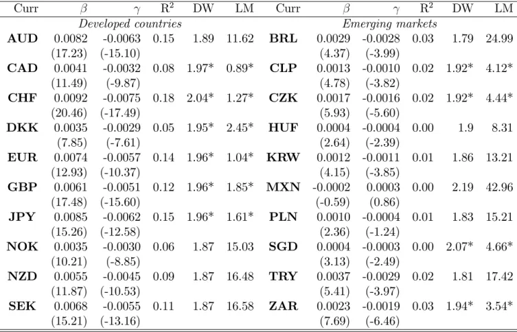
Table 3 reports the results from estimating regression (4), where FX returns are regressed on contemporaneous and lagged order ‡ow; the estimation is carried out by OLS and with standard errors calculated following Newey and West (1987). The coe¢ cients associated with contemporaneous ‡ow are generally positive and highly signi…cant. This was expected since the data set includes orders from institutional investors, which are big players in the market, so their order ‡ow is expected to move the market due to both information and trading volumes related to hedging. The exception is the MXN.7 In contrast, the coe¢ cients of lagged
6The standard errors of the estimates are calculated from the deviation of the estimates of the
cross-sectional regressions from their mean, as follows: 2([LIQm ) = M12 PM m=1([ LIQ m [LIQ)2; 2(\otherm ) = 1 M2 PM m=1(\ other m \other)2; 2("bi) = M12 PM
m=1("di;m "bi)2. We employ the portfolio construction tech-nique so that the estimates of the sensitivities of excess returns to the factors are more precise. However, when calculating the standard errors, we also employ the Shanken (1992) adjustment.
7Even though formally considered a ‡oating system, the Mexican peso arrangement might be a¤ected by
order ‡ow are negative and generally signi…cant, which is consistent with our priors since they capture the return reversal. For the currencies of the advanced economies, the regressions have particularly high explanatory power, exceeding 18% for CHF.
Insert Table 3 here
-Running the same regression for each independent month in the sample period gives a time series of monthly s for each currency. These series represent our monthly proxies of overall liquidity for the currencies considered.8 We then calculate a systematic (or aggregate) liquidity
measure from the liquidity measures of individual currencies. Indeed, given that there is a common component in the cost of providing liquidity in the FX market, it seems reasonable to expect the time-variation in liquidity to be correlated across currencies. The results of papers conducted on the stock market are supportive of this hypothesis. Regarding the FX market, Melvin and Taylor (2009) show a substantial shift in trading costs common across currencies during the last …nancial crisis. Focusing on the years of the last …nancial crisis (2007-2008), Mancini, Ranaldo, and Wrampelmeyer (2010) analyze common liquidity across 9 exchange rates employing the Pastor and Stambaugh measure and …nd a strong positive correlation in liquidity cross-sectionally. Given the particular market conditions in which the co-movement has been found, it does not follow that the same result can be generalized to normal market conditions. Since the data set analyzed here includes crisis and non-crisis periods, an answer to this question can be given irrespective of market conditions. Furthermore, our large number of currencies, including both developed and emerging countries, allows us to establish fairly robust and general results.
A preliminary analysis of the correlations between the individual liquidity innovation
mea-of the revenues from oil exports (Frankel and Wei (2007)).
8Overall, 79% of the betas are correctly signed (39% are also statistically signi…cant), and 76% of the
sures shows that 68% of the series are positively correlated and that over 22% of the corre-lations are statistically signi…cant. This is a …rst sign of the presence of a common liquidity component.
Next, we construct the common liquidity measure according to equations (6) to (8). The proxy captures the innovation in common liquidity across currencies. It presents a mean of -0.004% and a standard deviation of 0.219%. Furthermore, the proxy has an autocorrelation of about -13%. In Figure 1 we show the evolution over time of both the level of systematic liquidity and its innovation. Regression (9) is run to investigate the ability of the proxy to capture systematic liquidity across currencies. The regression is estimated by OLS and the standard errors are adjusted according to Newey and West (1987). The results are highly supportive of the presence of commonality (see Table 4). All the coe¢ cients are positive and statistically signi…cant, except CAD, BRL, and TRY. Furthermore, about 70% of the regressions have an R2 in excess of 5%. Hence, the common liquidity proxy does generally explain some fraction of the movements of individual currencies’liquidity.
Insert Table 4 here
-B
Is there a liquidity risk premium?
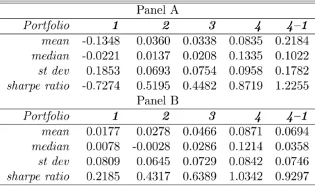
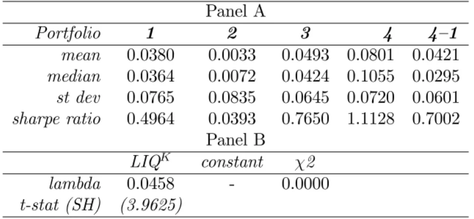
Next, we build four portfolios based on the ranking of the sensitivities of the currencies’returns to the common liquidity measure. This exercise reveals that portfolios with higher sensitivity dominate the ones with lower sensitivity to liquidity risk, as one would expect. Table 5 (Panel A) shows some descriptive statistics for the excess returns of the four portfolios. It includes in the last column the return of a strategy that goes long on the most sensitive portfolio and short on the least sensitive one. The spread in average returns is substantial and gives empirical support to the presence of a systematic liquidity risk premium.
In order to check whether the results of our analysis are driven by the Turkish lira extreme behavior during the 2001 crisis, we cap the monthly currencies’ returns and excess returns to +/- 10%.9 Table 5 (Panel B) shows that the most sensitive portfolios still receive higher
excess returns on average. This is also evident from the graphical analysis of the cumulative excess returns of the four portfolios in Figure 2.
Insert Table 5 here
-Rebalancing the portfolios at each year-end, we get a turnover of the currencies in the portfolios of about 37%. On average, emerging market currencies have a lower turnover than developed country ones. The currency with the lowest turnover is the NZD that has a highly positive sensitivity to innovations in market liquidity and stays in portfolio 4 for the whole sample period. The currencies with a low turnover are the CZK and the ZAR, that generally show negative sensitivities to innovations in market liquidity, and the BRL and HUF, that present positive sensitivities. Whereas the currencies with the higher turnover are the CHF, CLP, EUR, GBP, MXN, and SEK, whose returns are all generally positively correlated to innovations in market liquidity.
C
Liquidity risk: a priced common risk factor
Table 6 shows the results of the Fama-MacBeth procedure with di¤erent equation speci…ca-tions. Panel A reports the analysis with the systematic liquidity risk as common risk factor. The coe¢ cient associated with the systematic liquidity risk is positive and strongly statis-tically signi…cant. In particular, we estimate an annualized liquidity risk premium of around
9During 2001 and part of 2002, the Turkish crisis led to a collapse of the Turkish lira, that experimented
massive returns. In detail, during the year 2001, the monthly excess return of the USD/TRY was in excess of -50%.
4.7%.
What happens to the market price of liquidity risk when other sources of risk are included in the regression analysis? Panels B and C show the results with the inclusion of the dollar risk and the carry risk factors. In both cases, the associated with the systematic liquidity risk remains statistically signi…cant and does not change signi…cantly.
In Panel B, the dollar risk factor is signi…cant, so the result is not as strong as in Lustig, Roussanov, and Verdelhan (2010) where the dollar risk factor does not explain any of the cross-sectional variation of the portfolios’excess returns. Furthermore, as Lustig, Roussanov, and Verdelhan (2010), we do …nd that the sensitivities of the portfolios’ excess returns to the dollar risk factor are not di¤erent from one, so the inclusion of a constant in the cross-sectional regression is not appropriate.10 More clearly, Panel C shows that the carry risk
factor is not statistically signi…cant in explaining the cross-sectional variation of the liquidity-sorted portfolios’ excess returns, once introduced in the analysis together with the liquidity risk factor. Hence, we conclude that systematic liquidity risk is priced in the FX market.11
Insert Table 6 here
-In their analysis of liquidity across 9 developed countries’ currencies during the recent …nancial crisis, Mancini, Ranaldo, and Wrampelmeyer (2010) identify a liquidity risk premium as high as 20%. Our lower estimate of the liquidity risk premium can be explained by the inclusion in our sample of both crisis and non-crisis periods. From this comparison, we can
10These results are con…rmed in the analysis of Menkho¤, Sarno, Schmeling and Schrimpf (2011).
11We also considered the global FX volatility risk as a potential common risk factor. We construct this
factor as the absolute value of currency returns following Menkho¤, Sarno, Schmeling, and Schrimpf (2011). Estimating the lambda associated with the additional risk factor, we …nd that global FX volatility is not signi…cant in explaining the cross-section of the currencies excess returns. Furthermore, the inclusion of this additional risk factor makes the systematic liquidity risk factor statistically not signi…cant.
suggest that the FX liquidity risk premium is time-varying. Following the theoretical model developed by Vayanos (2004), the liquidity risk premium is time-varying due to the changes in investors’ liquidity preferences. In other words, during a …nancial crisis, investors’ need to liquidate their assets becomes more likely and leads to a higher liquidity risk premium. However, our results show that a liquidity risk premium is present and signi…cant in the FX market irrespective of the market conditions.
VI
FURTHER ANALYSIS
A
Liquidity risk premium: extension
Adjusting the CAPM for liquidity, Acharya and Pedersen (2005) extend the de…nition of liquidity risk to include the covariance of an individual asset liquidity and market liquidity, and the covariance of individual asset liquidity and the market return, in addition to the covariance of an asset return and market liquidity already presented by Pastor and Stambaugh (2003). Following their model, we extend our analysis to estimate liquidity risk as both the covariance of currencies return and market liquidity, and the covariance of currencies liquidity and market liquidity.12 The rationale behind this is that an investor requires a premium to hold a currency that is illiquid when the market as a whole is illiquid. As a consequence, expected currencies returns will be negatively correlated to the covariance of individual currencies liquidity and market liquidity.
Thus, the s measuring systematic liquidity risk are estimated from the following
regres-12We thus leave out the additional measure of liquidity risk, given by the covariance of innovations of
individual liquidity with the market return, since there is no stock market return equivalent for the FX market.
sions: erj;m = j + 1jDL C m+"j;m (16) DLj;m = 0j + 2jDL C m+"0j;m: (17)
The …rst regression is the equivalent of regression (11), with innovations in common liq-uidity as the only common risk factor. In addition, we run the second regression in order to estimate the Acharya and Pedersen (2005) additional measure of liquidity risk, given by the regression of innovations in individual liquidity on innovations in common liquidity.
Hence, our ‘net’ s measuring systematic liquidity risk are given by:
(18) bj =b1j b2j
At this point, we conduct the same empirical asset pricing analysis as above in equation (12) and we quantify this enhanced measure of liquidity risk.
The high signi…cance of the betas ( 2j) is a strong sign of the presence of a kind of liquidity risk not captured by the above measure alone ( 1j).
Table 7 shows the results of the extended analysis. For liquidity-sorted portfolios, the coe¢ cient is still positive and signi…cant. As in the previous case, the estimated annualized liquidity premium is above 4%. Overall, therefore, the results are qualitatively unchanged when allowing for the additional e¤ects in the de…nition of liquidity risk in Acharya and Pedersen (2005).
-B
Alternative liquidity measures
We extend our analysis of liquidity by building the proxy for liquidity from Kyle (1985)’s theoretical model (Evans and Lyons, 2002b). We employ it to calculate a measure of market liquidity and investigate the presence of a premium associated with its innovations. The con-temporaneous impact of order ‡ow on the exchange rate can be explained as the information discovery process of the dealer, who updates her quotes after receiving orders from her clients and other dealers. Nevertheless, the impact does not only re‡ect information arrival, but also the level of market liquidity. In fact, the contemporaneous impact, changed of sign, corre-sponds to the measure of market depth from Kyle (1985)’s model. So, we extend our analysis of liquidity by building this proxy as an alternative liquidity measure to the one in the main analysis.
Estimating regression (3) for every currency, for every month in the sample, we take the estimated coe¢ cient for changed of sign as our new measure of liquidity.13
(19) Lnewi;m = bi;m:
The rationale behind this proxy is that the more liquid a market, the lower the impact of transactions on an asset prices.
Table 8 shows the results of the portfolio and empirical asset pricing analysis conducted as in the main sections based on this new liquidity measure. Panel A reports some descriptive statistics of excess returns of the portfolios constructed from the ranking of the sensitivities of currencies to innovation in market liquidity. The results are qualitatively similar to the ones
13The higher the impact of transactions on prices, the lower the liquidity in the market. As a result, is a
measure of illiquidity. We change the sign of to takeLi;m as a measure of liquidity and make the measure comparable to the others in the paper.
obtained in our main results. This is also true for the liquidity risk premium (Panel B). We have estimated liquidity as the return reversal associated with order ‡ow. Practically, we have estimated liquidity as the impact of lagged order ‡ow on currency returns. In this section, following Pastor and Stambaugh (2003) we add lagged currency returns as an inde-pendent variable in the regression, to account for the possible e¤ects of serial correlation in currency returns. So we run the following regression using daily data for every month in the sample:
(20) ri;t = i+ i xi;t+ i xi;t 1+ iri;t 1+"i;t:
Hence, we take the estimated coe¢ cient for to be our new proxy for liquidity and we have a monthly liquidity series for each currency i:
(21) Li;m =bi;m:
Next, we use these new estimates of liquidity to calculate the innovation in common liquid-ity from equations (7)-(9) and conduct the same portfolio and empirical asset pricing analysis. The results of these analysis are reported in Table 9. The portfolio analysis shows that there still exist a spread between the portfolios that contain the less and more sensitive currencies to innovation in common liquidity (Panel A). Furthermore, the empirical asset pricing exercise con…rms the presence of a liquidity risk premium (Panel B).
C
Emerging market currencies
In FX market most of the trading happens between the currencies of the most developed countries. If the currencies of emerging markets are less liquid, are their returns also more
sensitive to unexpected changes in market liquidity?
Since our broad data set includes a number of emerging market and less traded currencies, it is interesting to conduct our analysis excluding the most traded currencies (AUD, CAD, CHF, GBP, EUR, JPY, NZD, and SEK). So, in this section we review the results of our portfolio analysis and empirical asset pricing exercise limiting the currencies included in our data set to the BRL, CLP, CZK, DKK, HUF, KRW, MXN, NOK, PLN, SGD, TRY, and ZAR. In detail, we group the 12 currencies in 4 portfolios with 3 currencies in each one and conduct the same analysis as the core one.
As we expect, the spread between the excess return of the portfolios is higher once the most traded currencies are excluded from our sample (Table 10 Panel A). Furthermore, the liquidity risk premium associated with this sample is signi…cantly higher, exceeding the value of 7% (Table 10 Panel B). So, liquidity is more important in pricing the cross-section of emerging market and less traded developed ones currency excess return.
D
Crisis period
In this section we are extending our analysis to the recent …nancial crisis period, focusing our attention on the period after Lehman Brothers collapse in September 2008. Our transaction data set does not allow us to analyze this period, so we employ a di¤erent data set. Log returns and excess returns are calculated from the FX spot and forward exchange rates of the US dollar versus the currencies and are the WM/Reuters Closing Rates obtained from Datastream. The order ‡ow data comes from proprietary daily transactions between end-user segments and UBS, one of the world’s largest player in the FX market. It includes daily transaction data of UBS with four di¤erent segments: asset managers, hedge funds, corporate and private clients. At the end of each business day, transactions registered at any world-wide
o¢ ce are aggregated across segments. The order ‡ow data measures the imbalance between the value of purchase and sale orders for foreign currency initiated by clients. In detail, it includes the transactions against the USD of developed country currencies AUD, CAD, CHF, EUR, GBP, JPY, NOK, NZD, SEK and emerging market currencies BRL, KRW, MXN, SGD, and ZAR, measured in billions of US dollars. The sample period is from January 1, 2005 until May 27, 2011.
The order ‡ow data analyzed in this section is di¤erent from the one in the main analysis in some respects. It includes a more limited part of the FX market, namely clients of UBS. In addition, the data set includes the transactions of 9 developed countries and 4 emerging markets currencies against the USD. As a result, the measure of market liquidity calculated from this sample will be more limited in its broadness comparing it to the global FX measure built in our main analysis. However, this data set covers a period of more than 6 years across the recent …nancial crisis. As a consequence, we are able to conduct a portfolio analysis to investigate the presence of a liquidity risk premium during the recent …nancial crisis. Nev-ertheless, the relative smaller length and cross-section do not allow us to conduct an asset pricing exercise, thus we are not estimating a liquidity risk premium.
Turning to the empirical results, after the collapse of Lehman Brothers, a signi…cant shock to liquidity in the FX market took place together with a subsequent increase in volatility (Panel A of Figure 3). Furthermore, there is strong evidence of a sharp increase in the spread in the excess returns between the portfolios containing the three less and most sensitive currencies to innovation in common liquidity after the collapse of Lehman Brothers. Table 11 reports the descriptive statistics of the excess returns of the portfolio containing the less sensitive currencies to innovation in common liquidity and the portfolio containing the three most sensitive ones. The average excess returns and the Sharpe ratios suggest the presence of a
premium in the portfolios depending on the higher liquidity risk on the second portfolio. This can be even more clearly seen in the graphical analysis of the cumulative excess returns of the two portfolios in Panel B of Figure 3, where there is an evident widening in the spread after the Lehman collapse, consistent with an increased premium required for liquidity risk.
In conclusion, this section provides evidence of the presence of a liquidity risk premium during the latest …nancial crisis period. Even though we are not able to quantify a premium, our portfolio analysis shows empirical support for a widening in the spread in excess returns between the portfolio less exposed to liquidity risk and the one most exposed.
VII
ROBUSTNESS CHECKS
A
Volume-weighted common liquidity
In the calculation of a common component in liquidity across currencies, we have taken the average of equally weighted currencies. In this section we calculate the common component in liquidity across currencies by weighting the currencies based on their share of market turnover. We take the monthly weights as the annual percentages of the global foreign exchange market turnover by currency pair reported by in the Triennial reports of the BIS for various years (1995, 1998, 2001, 2004, 2007, and 2010). We calculate the weights for the years not covered by the reports by interpolation. Furthermore, for the currencies not individually included in the reports, we take the value of "other currencies versus the USD" and evenly distribute it among these currencies.
In detail, taking the measures of changes in liquidity of individual currencies DLi;m from equation (6), the new measure of changes in market liquidity (DLm) is calculated as:
(22) DLm = 1 N N X i=1 wi;mDLi;m:
Where wi;m is the weight associated with currency i in month m.14 Then we proceed to estimate the innovation in market liquidity running regression (8).
The new measure of innovation in market liquidity presents a correlation of 67% with the one from our core analysis.
Next, we conduct the same portfolio analysis as in the main section. The results show the presence of a high spread between the excess returns of the portfolios with lower and higher sensitivities to innovation in market liquidity (Table 12). Thus, the results do not qualitatively change once the weighting is introduced in the calculation of market liquidity.
B
Di¤erent rebalancing horizons
Our portfolio analysis results are based on a yearly rebalancing of the portfolios. In this section, in order to pick up the great variability in the innovation in common liquidity as shown in Figure 1, we rebalance the portfolios at higher frequencies, 3 months or 1 month. In Table 13 we report the results of the same analysis conducted with a di¤erent rebalancing period. Starting from January 1999, we rank the currencies at every end of a 3-month or 1-month period based on their historical sensitivity to innovation in market liquidity. After grouping the currencies in 4 portfolios according to this ranking, we construct a series of excess returns for the portfolios for the following 3-month or 1-month period. Table 13 show that the portfolio analysis does not change dramatically once the rebalancing is conducted at higher
14The currencies with the highest weights are the EUR (37%), the JPY (20%), and the GBP (12%). The
other developed country currencies (AUD, CAD, and CHF) have weights of around 5%. All the other currencies have lower weights.
frequencies (Panel A and Panel C). The portfolio containing the most sensitive currencies is still presenting higher excess returns than the one containing the less sensitive currencies. Furthermore, the annualized liquidity risk premium stays around 4% for both rebalancing frequencies (Panel B and Panel D). So, we can conclude that our results are not due to a speci…c rebalancing time frame.
C
GMM alternative estimation
In our main section we estimate the premium associated with our liquidity risk factor using the Fama-MacBeth procedure. In this section, we conduct the same estimation via the General Method of Moments procedure as a robustness check of our results. As discussed in the empirical asset pricing section above, our problem can be represented as:
(23) E[erj;t] = j:
In fact, given the no-arbitrage condition, the currencies excess returns have a zero price:
(24) E[mt+1erj;t+1] = 0:
With the pricing kernelmt= 1 bf(ft f):Whereft is the liquidity risk factor,bf is the factor loading, and f is the factor mean.
We conduct a two-step GMM estimation with an identity matrix as our …rst-step weighting matrix and the following six moment conditions to estimate our three parametersbf, f, and
(25) 2 6 6 6 6 6 6 4 (1 bf(fm f))erj;m fm f (fm f)0(fm f) vf 3 7 7 7 7 7 7 5
Where vf is the factor variance. After estimating the three factor, we proceed to estimate , the market price of risk, from the relation = bfvf. The associated standard errors are calculated via the Delta method. Since we are estimating 3 parameters by minimizing a system of six equations, we run the J-test for overidentifying restrictions.
Table 14 reports the results. The liquidity risk premium estimated via GMM is lower but still signi…cant. Furthermore, the loading associated with the liquidity risk factor is statistically signi…cant as well.
VIII
CONCLUSIONS
In this paper, we study liquidity in the FX market of 20 US dollar exchange rates over 14 years. De…ning liquidity as the expected return reversal associated with order ‡ow, the well-known Pastor-Stambaugh measure for stocks, we estimate individual currency liquidity measures. As for the stock market, we observe that the individual FX liquidity measures are correlated across currencies. We document the presence of a common component in liquidity across currencies, which is consistent with the literature that identi…es the dealers’inventory control constraints and preferences as signi…cant channels in‡uencing price formation. In fact, some of the dealers’ considerations regarding their inventory positions may be irrespective of the particular currencies involved in the trades. In other words, the dealers’ response to incoming orders of di¤erent currencies has a common part dictated by their inventory position considerations. Furthermore, the commonality can be explained by the need for
funding liquidity on the side of traders. In this sense, changes in the funding conditions a¤ect the provision of liquidity in all the currencies in which an investor trades.
The aggregate liquidity measure exhibits strong variation through time. Our focus in this paper is on unexpected changes in aggregate liquidity. In this sense, the paper’s main contribution is the identi…cation and estimation of a systematic liquidity risk premium that signi…cantly explains part of the cross-section variation in exchange rates.
If there is a liquidity risk premium in the FX market, an investor will require a higher return to hold a currency more sensitive to unexpected liquidity. The higher is the sensitivity of a currency to innovations in liquidity, the greater is the premium for holding that currency. Taking the perspective of a US investor, we group the currencies in 4 portfolios based on the historical currencies’sensitivities to the liquidity measures. Comparing the returns of the portfolios, we …nd that the returns are higher for the portfolios containing the more sensitive currencies.
At this stage, to verify whether the sensitivity of the currencies to innovations in liquidity is indeed priced in the market, we perform standard asset pricing tests. Applying the Fama-MacBeth procedure to a cross-section of liquidity-sorted portfolios, we estimate an annualized systematic liquidity risk premium around 4.7%. Furthermore, we control for other variables as a source of risk that can potentially explain variation in the cross-section of currency returns. The results do not change: the liquidity risk factor stays signi…cant even after taking into account the dollar risk and the carry risk factors. In addition, we extend the de…nition of liquidity risk to include the commonality in liquidity, and con…rm a positive and signi…cant liquidity risk premium. Furthermore, we …nd our results to be robust to a series of tests, including the volume-weighting of currencies for the construction of the common liquidity measure, changing the rebalancing horizon, and estimating the premium with an alternative
estimation method. Therefore, we can conclude that liquidity risk is a priced factor in the cross-section of currency returns and that it is both statistically and economically signi…cant. Furthermore, our broad data set allow us to conduct a detailed analysis of the behavior of emerging market currencies. We …nd that liquidity risk is especially important in explaining the cross-section of emerging market currencies. Indeed, excluding the most traded currencies, the liquidity risk premium reaches 7%, which is sensibly higher than the one for the whole data set. As a consequence, while signi…cant for the cross-section of the whole data set, global liquidity risk is especially important for emerging market currencies.
Finally, employing a di¤erent data set, we …nd empirical support through the portfolio analysis of the increase in the magnitude of the liquidity risk premium after the collapse of Lehman Brothers in the recent …nancial crisis.
A
Appendix: ABBREVIATIONS
List of the abbreviations used in the paper for currencies: AUD: Australian dollar
BRL: Brazilian real CAD: Canadian dollar CHF: Swiss franc CLP: Chilean peso CZK: Czech koruna DKK: Danish krone DM: Deutsche mark EUR: euro
GBP: Great Britain pound HUF: Hungarian forint JPY: Japanese yen KRW: Korean won MXN: Mexican peso NOK: Norwegian kroner NZD: New Zealand dollar PLN: Polish zloty
SEK: Swedish krona SGD: Singapore dollar TRY: Turkish lira
USD: United States dollar ZAR: South African rand
References
Acharya, V. V., and L. H. Pedersen. "Asset Pricing with Liquidity Risk."Journal of Financial Economics, 77 (2005), 375-410.
Admati, A. R., and P. P‡eiderer. "A Theory of Intraday Patterns: Volume and Price Vari-ability." The Review of Financial Studies, 1 (1988), 3-40.
Amihud, Y. "Illiquidity and Stock Returns: Cross-Section and Time Series E¤ects." Journal of Financial Markets, 5 (2002), 31-56.
Amihud, Y., and H. Mendelson. "Dealership Market: Market Making with Inventory."Journal of Financial Economics, 8 (1980), 31-53.
Amihud, Y., and H. Mendelson. "Asset Pricing and the Bid-Ask Spread."Journal of Financial Economics, 17 (1986), 223-249.
Amihud, Y., and H. Mendelson. "Liquidity, Maturity, and the Yields on U.S. Treasury Secu-rities." Journal of Finance, 46 (1991), 1411-1425.
Asparouhova, E.; H. Bessembinder; and I. Kalcheva. "Liquidity Biases in Asset Pricing Tests."
Journal of Financial Economics, 96 (2010), 215-237.
Bank for International Settlements. Triennial Central Bank Survey of Foreign Exchange and
Derivatives Market Activity in April 2010 - Preliminary Global Results. September (2010).
Bekaert, G.; C. R. Harvey; and C. Lundblad. "Liquidity and Expected Returns: Lessons from Emerging Markets." Review of Financial Studies, 20 (2007), 1784-1831.
Bessembinder, H. "Bid-Ask Spreads in the Interbank Foreign Exchange Markets."Journal of Financial Economics, 35 (1994), 317-348.
Bessembinder, H.; K. Chan; and P. Seguin. "An Empirical Examination of Information, Di¤er-ences of Opinion, and Trading Activity."Journal of Financial Economics, 40 (1996), 105-134. Bjønnes, G. H., and D. Rime. "Dealer Behavior and Trading Systems in Foreign Exchange Markets." Journal of Financial Economics, 75 (2005), 571-605.
Bollerslev, T., and M. Melvin. "Bid-ask Spreads and Volatility in the Foreign Exchange Mar-ket." Journal of International Economics, 36 (1994), 355-372.
Brennan, M. J.; T. Chordia; and A. Subrahmanyam. "Alternative Factor Speci…cations, Secu-rity Characteristics, and the Cross-section of Expected Stock Returns."Journal of Financial Economics, 49 (1998), 345-373.
Brennan, M. J., and A. Subrahmanyam. "Market Microstructure and Asset Pricing: On the Compensation for Illiquidity in Stock Returns." Journal of Financial Economics, 41 (1996), 441-464.
Brunnermeier, M. K., and L. H. Pedersen. "Market Liquidity and Funding Liquidity." The Review of Financial Studies, 22 (2009), 2201-2238.
Campbell, J.; S. J. Grossman; and J. Wang. "Trading Volume and Serial Correlation in Stock Returns."Quarterly Journal of Economics, 108 (1993), 905-939.
Chen, J. "Pervasive Liquidity Risk and Asset Pricing." Mimeo, Columbia Business School (2005).
Cheung, Y., and M. D. Chinn. "Currency Traders and Exchange Rate Dynamics: A Survey of the U.S. Market."Journal of International Money and Finance, 20 (2001), 439-471. Chordia, T.; R. Roll; and A. Subrahmanyam. "Commonality in Liquidity."Journal of Finan-cial Economics, 56 (2000), 3-28.
Chordia, T.; R. Roll; and A. Subrahmanyam. "Market Liquidity and Trading Activity." Jour-nal of Finance, 56 (2001), 501-530.
Copeland, T. E., and D. Galai. "Information E¤ects on the Bid-Ask Spread." Journal of
Finance, December, 38 (1983), 1457-1469.
Datar, V. T.; N. Y. Naik; and R. Radcli¤e. "Liquidity and Stock Returns: An Alternative Test."Journal of Financial Markets, 1 (1998), 203-219.
De Long, J. B.; A. Shleifer; L. H. Summers; and R. J. Waldmann. "Noise Trader Risk in Financial Markets."Journal of Political Economy, 98 (1990), 703-738.
Evans, M. D. D., and R. K. Lyons. "Order Flow and Exchange Rate Dynamics." Journal of Political Economy, 110 (2002a), 170-180.
Evans, M. D. D., and R. K. Lyons. "Time-Varying Liquidity in Foreign Exchange." Journal
of Monetary Economics, 49 (2002b), 1025-1051.
Evans, M. D. D., and R. K. Lyons. "Understanding Order Flow." International Journal of Finance & Economics, 11 (2006), 3-23.
Fama, E. F., and J. D. MacBeth. "Risk, Return, and Equilibrium: Empirical Tests." Journal of Political Economy, 81 (1973), 607-636.
Frankel, J. A., and S. Wei. "Estimation of De Facto Exchange Rate Regimes: Synthesis of the Techniques for Inferring Flexibility and Basket Weights." NBER working paper (2007), 14016.
Froot, K. A., and T. Ramadorai. "Currency Returns, Intrinsic Value, and Institutional-Investor Flows." Journal of Finance, 60 (2005), 1535-1566.
Gehrig, T., and L. Menkho¤. "The Use of Flow Information in Foreign Exchange Markets: Exploratory Evidence."Journal of International Money and Finance, 23 (2004), 573-594.
Glosten, L. R., and P. R. Milgrom. "Bid, Ask, and Transaction Prices in a Specialist Market with Heterogeneously Informed Traders." Journal of Financial Economics, 14 (1985), 71-100.
Goodhart, C. "The Foreign Exchange Market: A Random Walk with a Dragging Anchor."
Economica, 55 (1988), 437-460.
Grossman, S. J., and M. H. Miller. "Liquidity and Market Structure." Journal of Finance, 43 (1988), Papers and Proceedings of the Forty-Seventh Annual Meeting of the American Finance Association, Chicago, Illinois, December 1987, 617-633.
Harris, L. "Statistical Properties of the Roll Serial Covariance Bid/Ask Spread Estimator."
Journal of Finance, 45 (1990), 579-590.
Hasbrouck, J. "Trading Costs and Returns for U.S. Equities: Estimating E¤ective Costs from Daily Data."Journal of Finance, 64 (2009), 1445-1477.
Hasbrouck, J., and D. J. Seppi. "Common Factors in Prices, Order Flows, and Liquidity."
Journal of Financial Economics, 59 (2001), 383-411.
Ho, T., and H. R. Stoll. "Optimal Dealer Pricing Under Transactions and Return Uncertainty."
Journal of Financial Economics, 9 (1981), 47-73.
Hsieh, D. A., and A. W. Kleidon. "Bid-Ask Spreads in Foreign Exchange Markets: Impli-cations for Models of Asymmetric Information." In The Microstructure of Foreign Exchange
Markets, J. A. Frankel; G. Galli; and A. Giovannini, eds. National Bureau of Economic
Huberman, G., and D. Halka. "Systematic Liquidity." Journal of Financial Research, 24 (2001), 161-178.
International Monetary Fund.World Economic Outlook. April (2010).
Killeen, W. P.; R. K. Lyons; and M. J. Moore. "Fixed versus Flexible: Lessons from EMS Order Flow." Journal of International Money and Finance, 25 (2006), 551-579.
Korajczyk, R. A., and R. Sadka. "Pricing the commonality across alternative measures of liquidity." Journal of Financial Economics, 87 (2008), 45-72.
Kyle, A. S. "Continuous Actions and Insider Trading." Econometrica, 53 (1985), 1315-1335.
Lee, T. "Spread and Volatility in Spot and Forward Exchange Rates."Journal of International
Money and Finance, 13 (1994), 375-383.
Lee, K. "The World Price of Liquidity Risk." Journal of Financial Economics, 99 (2011), 136-161.
Lesmond, D. A. "Liquidity of Emerging Markets."Journal of Financial Economics,77 (2005), 411–452.
Lesmond, D. A.; J. P. Ogden; and C. Trzcinka. "A New Estimate of Transaction Costs."
Review of Financial Studies, 12 (1999), 1113-1141.
Lustig, H.; N. Roussanov; and A. Verdelhan. "Common Risk Factors in Currency Markets." Mimeo (2010).
Lustig, H., and A. Verdelhan. "The Cross Section of Foreign Currency Risk Premia and Consumption Growth Risk." The American Economic Review, 97 (2007), 89-117.
Lyons, R. K. "Tests of Microstructural Hypotheses in the Foreign Exchange Market."Journal of Financial Economics, 39 (1995), 321-351.
Lyons, R. K. "A Simultaneous Trade Model of the Foreign Exchange Hot Potato."Journal of International Economics, 42 (1997), 275-298.
Lyons, R. K. The Microstructure Approach to Exchange Rates. MIT Press (2001).
Mancini, L.; A. Ranaldo; and J. Wrampelmeyer. "Liquidity in the Foreign Exchange Market: Measurement, Commonality, and Risk Premiums." Mimeo (2011).
Melvin, M., and M. P. Taylor. "The crisis in the foreign exchange market."Journal of
Inter-national Money and Finance, 28 (2009), 1317-1330.
Menkho¤, L.; L. Sarno; M. Schmeling; and A. Schrimpf. "Carry Trades and Global Foreign Exchange Volatility."Journal of Finance, forthcoming (2011).
Naes, R.; J. A. Skjeltorp; and B. A. Ødegaard. "Stock Market Liquidity and the Business Cycle." Journal of Financ