Continuous dimensional emotion tracking in music

C

ontinuous

D

imensional

E

motion

T

racking in

M

usic

Vaiva Imbrasait ˙e

April

2015

University of Cambridge

Computer Laboratory

Downing College

D

eclaration

This dissertation is the result of my own work and includes nothing which is the outcome of work done in collabora-tion except as declared in the Preface and specified in the text.

It is not substantially the same as any that I have submit-ted, or, is being concurrently submitted for a degree or dip-loma or other qualification at the University of Cambridge or any other University or similar institution except as de-clared in the Preface and specified in the text. I further state that no substantial part of my dissertation has already been submitted, or, is being concurrently submitted for any such degree, diploma or other qualification at the University of Cambridge or any other University of similar institution except as declared in the Preface and specified in the text This dissertation does not exceed the regulation length of

S

ummary

The size of easily-accessible libraries of digital music recordings is growing every day, and people need new and more intuitive ways of managing them, search-ing through them and discoversearch-ing new music. Musical emotion is a method of classification that people use without thinking and it therefore could be used for enriching music libraries to make them more user-friendly, evaluating new pieces or even for discovering meaningful features for automatic composition.

The field of Emotion in Music is not new: there has been a lot of work done in musicology, psychology, and other fields. However, automatic emotion prediction in music is still at its infancy and often lacks that transfer of knowledge from the other fields surrounding it. This dissertation explores automatic continuous dimensional emotion prediction in music and shows how various findings from other areas of Emotion and Music and Affective Computing can be translated and used for this task.

There are four main contributions.

Firstly, I describe a study that I conducted which focused on evaluation met-rics used to present the results of continuous emotion prediction. So far, the field lacks consensus on which metrics to use, making the comparison of dif-ferent approaches near impossible. In this study, I investigated people’s intuit-ively preferred evaluation metric, and, on the basis of the results, suggested some guidelines for the analysis of the results of continuous emotion recognition al-gorithms. I discovered that root-mean-squared error (RMSE) is significantly prefer-able to the other metrics explored for the one dimensional case, and it has similar preference ratings to correlation coefficient in the two dimensional case.

Secondly, I investigated how various findings from the field of Emotion in Music can be used when building feature vectors for machine learning solutions to the problem. I suggest some novel feature vector representation techniques, testing them on several datasets and several machine learning models, showing the ad-vantage they can bring. Some of the suggested feature representations can reduce RMSE by up to 19% when compared to the standard feature representation, and

up to10-fold improvement for non-squared correlation coefficient.

Thirdly, I describe Continuous Conditional Random Fields and Continuous Condi-tional Neural Fields (CCNF) and introduce their use for the problem of continuous dimensional emotion recognition in music, comparing them with Support Vector Regression. These two models incorporate some of the temporal information that the standard bag-of-frames approaches lack, and are therefore capable of improv-ing the results. CCNF can reduce RMSE by up to20% when compared to Support

Vector Regression, and can increase squared correlation for the valence axis by up to40%.

Finally, I describe a novel multi-modal approach to continuous dimensional music emotion recognition. The field so far has focused solely on acoustic analysis of

The separation of music and vocals can improve the results by up to10% with a

stronger impact on arousal, when compared to a system that uses only acoustic analysis of the whole signal, and the addition of the analysis of lyrics can provide a similar improvement to the results of the valence model.

A

cknowledgements

First of all, I would like to thank the Computer Laboratory for creating a wonder-ful place to do your PhD in. The staff have always been more than accommod-ating with all of our requests and extremely helpful in any way they could be. I would like to thank the Student Admin and Megan Sammons in particular for being passionate about undergraduate teaching and creating opportunities for us to contribute. I want to thank the System Administrators and Graham Titmus in particular for being ever so helpful with any sort of technical problems. And also my biggest thanks to Mateja Jamnik for making women@CL happen and all the opportunities and support that it provides.

I am grateful for my research group—I feel very lucky to have chosen it, and to have been surrounded by a group of amazing people. Our daily coffee breaks were an anchor in my life and I will miss them greatly. I would like to give special thanks to Ian, for keeping me sane through the write-up, Tadas, as without him some of the work described here could never have happened, Leszek, for so many things that would not fit on this page, Luke, for many interesting conversations, Marwa, for being a wonderful officemate and for comparing notes on writing up and to everyone else in the group—you are all great. Many thanks to Alan for interesting discussions, Neil, for always making my day a little brighter, and, of course, my supervisor Peter Robinson for all the opportunities he created for me. My viva turned out to be a lot less scary and a lot more enjoyable than I expected. I would like to thank my examiners, Neil Dodgson and Roddy Cowie, for a very interesting discussion about my work. The feedback I got helped me put my work in perspective and make some important improvements to this dissertation. Your comments were greatly appreciated!

I would also like to thank my first IT teacher Agn ˙e Zlatkauskien ˙e, who spotted me in our extracurricular classes and decided to teach a12-year old girl to program.

If not for her, I might not be where I am now—the world would be a better place if there were more teachers like her.

Finally, I would like to thank my parents, who failed to tell me that Mathematics and then Computer Science are not girly subjects, and who supported me all the way through. I hope I have made you proud.

C

ontents

1. Introduction 19

1.1. Motivation and approach. . . 19

1.2. Research areas and contributions. . . 20

1.3. Structure. . . 21

1.4. Publications. . . 23

2. Background 25 2.1. Affective Computing. . . 25

2.1.1 Affect representation . . . 26

2.1.2 Facial expression analysis . . . 27

2.1.3 Emotion in voice . . . 28

2.1.4 Sentiment analysis in text . . . 30

2.2. Music emotion recognition. . . 33

2.2.1 Music and emotion . . . 33

2.2.2 Type of emotion. . . 34

2.2.3 Emotion representation. . . 34

2.2.4 Source of features. . . 36

2.2.5 Granularity of labels. . . 37

2.2.6 Target user . . . 37

2.2.7 Continuous dimensional music emotion recognition. . . 38

2.2.8 Displaying results. . . 39

2.3. Music emotion recognition challenges. . . 43

2.4. Datasets. . . 44

2.4.1 MoodSwings. . . 44

2.4.2 MediaEval2013. . . 45

2.4.3 MediaEval2014. . . 46

3. Evaluation metrics 47 3.1. Evaluation metrics in use. . . 47

3.1.2 Emotion recognition from audio/visual clues. . . 49

3.1.3 Emotion recognition from physiological cues. . . 50

3.1.4 Sentiment analysis in text . . . 50

3.1.5 Mathematical definition. . . 50

3.1.6 Correlation between different metrics. . . 52

3.1.7 Defining a sequence . . . 53

3.2. Implicitly preferred metric. . . 54

3.2.1 Generating predictions. . . 54

3.2.2 Optimising one metric over another. . . 55

3.2.3 Experimental design. . . 55

3.2.4 Results. . . 58

3.2.5 Discussion. . . 61

3.3. Conclusions. . . 63

4. Feature vector engineering 65 4.1. Features used. . . 65

4.1.1 Chroma. . . 66

4.1.2 MFCC. . . 67

4.1.3 Spectral Contrast. . . 69

4.1.4 Statistical Spectrum Descriptors. . . 70

4.1.5 Other features. . . 70

4.2. Methodology and the baseline method. . . 72

4.2.1 Album effect. . . 73

4.2.2 Evaluation metrics. . . 74

4.2.3 Feature sets. . . 74

4.3. Time delay/future window. . . 74

4.4. Extra labels. . . 76

4.5. Diagonal feature representation. . . 76

4.6. Moving relative feature representation. . . 77

4.7. Relative feature representation. . . 78

4.8. Multiple time spans. . . 80

4.9. Discussion. . . 81

4.10. Conclusions. . . 81

5. Machine learning models 83 5.1. Support Vector Regression . . . 84

5.1.1 Model description. . . 84

5.1.2 Kernels. . . 88

5.1.3 Comparison. . . 89

5.2. Continuous Conditional Random Fields. . . 91

5.2.1 Model definition. . . 91

Contents

5.2.3 Learning. . . 93

5.2.4 Inference. . . 94

5.3. Continuous Conditional Neural Fields. . . 94

5.3.1 Model definition. . . 95

5.3.2 Learning and Inference . . . 96

5.4. Comparison. . . 97

5.4.1 Design of the experiments. . . 97

5.4.2 Feature fusion . . . 99 5.4.3 Results. . . 99 5.4.4 Model-level fusion. . . .103 5.5. MediaEval2014. . . .103 5.6. Discussion. . . .105 5.6.1 Other insights. . . .105 5.7. Conclusion. . . .106 6. Multi modality 109 6.1. Separation of vocals and music. . . .109

6.1.1 Separation methods. . . .109 6.1.2 Methodology. . . .112 6.1.3 Results. . . .112 6.1.4 Conclusions. . . .116 6.2. Lyrics. . . .116 6.2.1 Techniques . . . .117 6.2.2 Methodology. . . .120 6.2.3 Results. . . .122 6.2.4 Conclusions. . . .130

6.3. Fully multi-modal system. . . .131

6.3.1 Methodology. . . .131 6.3.2 Results. . . .132 6.4. Conclusions. . . .136 7. Conclusion 139 7.1. Contributions. . . .139 7.1.1 Evaluation metrics. . . .139

7.1.2 Balance between ML and feature vector engineering. . . .139

7.1.3 Multi-modality . . . .140

7.2. Limitations and future work. . . .140

7.2.1 Online data. . . .140

7.2.2 Popular music. . . .140

7.2.3 Current dataset. . . .141

7.2.4 Imperfection of analysis. . . .141

Bibliography 145

F

igures

2.1. Image of the arousal-valence space with the appropriate emotion

labels, based onRussell[1980].. . . 27 2.3. An example of a one dimensional representation of emotion

predic-tion over time, where time is shown on the horizontal axis, and the dimension in question is represented by the vertical axis. . . 39 2.4. An example of a two dimensional representation of emotion

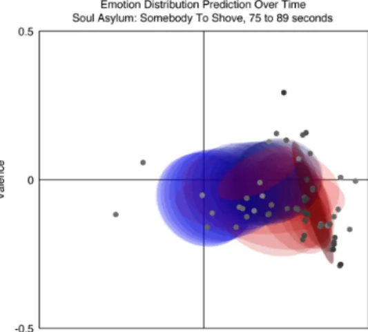
pre-diction over time (valence on the vertical axis and arousal on the horizontal axis), taken fromSchmidt et al.[2010], where time is rep-resented by the darkness of the dots (labels), or the color of the ellipses (distributions). . . 40 2.5. An example of a2.5 dimensional representation of emotion

predic-tion over time (height represents the intensity of emopredic-tion and colour is an interpolation between red-green axis of valence and yellow-blue axis of arousal with time on the horizontal axis), taken from Cowie et al.[2009] . . . 40 2.2. Summary of the various choices that need to be made for emotion

recognition in music. . . 42 2.6. Labeling examples for songs (from left to right) “Collective Soul

-Wasting Time”, “Chicago - Gently I’ll Wake You” and “Paula Abdul - Opposites Attract”. Each color corresponds to a different labeller

labelling the same excerpt of a song. . . 45 3.1. Scatter plots of relationships between metrics when comparing a

noisy synthetic prediction with ground truth. Notice how Euclidean, KL-divergence and RMSE are related.. . . 53 3.2. Example of a predictor with different correlation scores depending

on how sequence is defined. Blue is the ground truth data, red is a hypothetical prediction. For this predictor if we take the overall sequence as one the correlation score r = 0.93, but if we take cor-relations of individual song extracts (18 sequences of15 time-steps

each) the averager =0.45. . . 54 3.3. Sample synthetic traces. Blue is the ground truth, Red has a great

correlation score (0.94), but bad RMSE (81.56), and green has a low

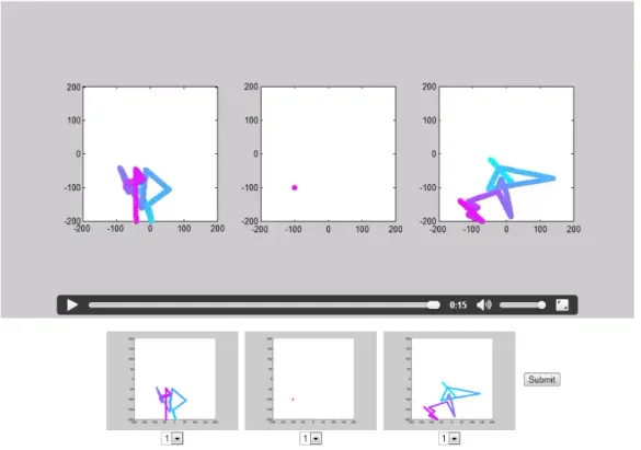
3.4. Screenshot of the study page. Instruction at the top, followed by a

video and the static emotion traces. . . 56

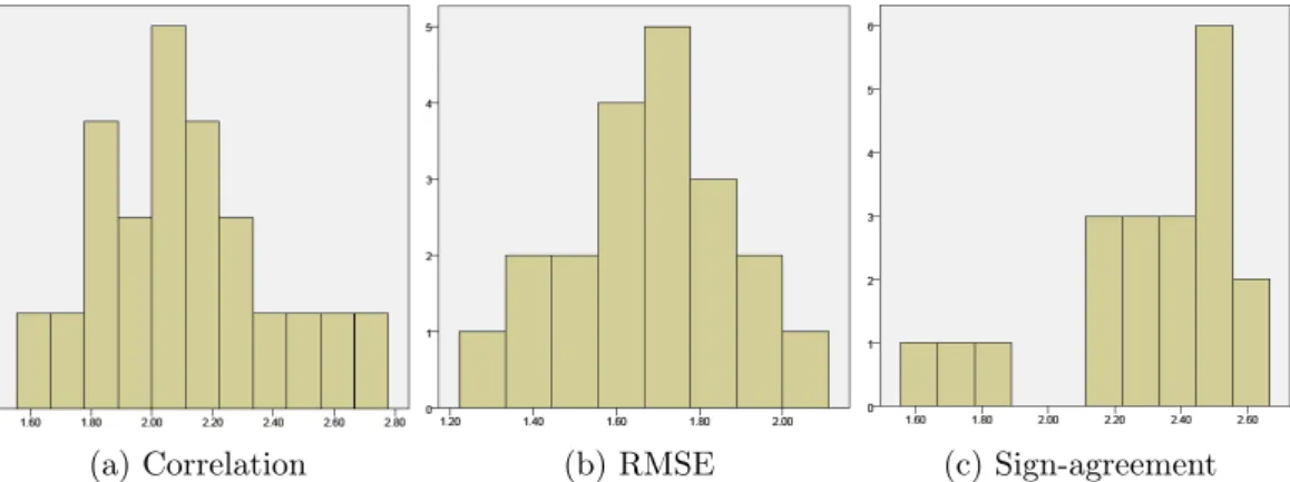
3.5. Arousal distributions for the three metrics. . . 59

3.6. Valence distributions for the three metrics. . . 59

3.7. Average ranking of the three tasks. RMSE Correlation SAGR KL-divergence . . . 60

3.8. 2D-task distributions for the three metrics. . . 60

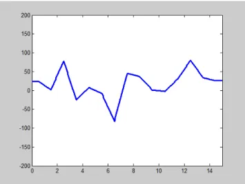
3.9. Example valence trace of a song used in the experiment. . . 62

4.1. An image of a spectrogram of a song . . . 67

4.2. An image of a chromagram of a song. . . 67

4.3. An image of the MFCC of a song. . . 68

5.1. A diagram depicting an example of linear classification. The dashed lines represent the maximum margin lines with the solid red line representing the separation line.. . . 84

5.2. A diagram depicting an example of non-linear classification. The solid red line represents the best non-linear separation line, while a linear separation without any errors is not possible in this example.. . 89

5.3. Graphical representation of the CCRF model. x_i represents the the ithobservation, andyiis the unobserved variable we want to predict. Dashed lines represent the connection of observed to unobserved variables (f is the vertex feature). The solid lines show connections between the unobserved variables (edge features).. . . 92

5.4. Linear-chain CCNF model. The input vector x_i is connected to the relevant output scalar yi through the vertex features that combine the hi neural layers (gate functions) and the vertex weights α. The outputs are further connected with edge featuresg_k . . . 94

6.1. A histogram showing the proportion of extracts that contain lyrics in the reduced MoodSwings dataset.. . . .123

6.2. A histogram showing the distribution of the number of words present in a second of a song in the reduced MoodSwings dataset.. . . .123

T

ables

2.1. Suggested set of musical features that affect emotion in music

(ad-apted fromGabrielsson and Lindström[2010]). . . 41 3.1. Summary of metrics used for evaluation of continuous emotion

prediction—music research at the top and facial expressions at the bottom. Starred entries indicate that the sequence length used in the paper was not made clear and the entry in the table is speculated . . . . 48 4.1. Artist-, album- and song-effect in the original MoodSwings dataset.. . 73 4.2. Comparison of the standard featureset extracted from MoodSwings

dataset and one extracted using OpenSMILE script using the baseline SVR model . . . 74 4.3. Results for the time delay/future window feature representation,

standard and short metrics . . . 76 4.4. Results for the presence of the extra label in the feature vector,

stand-ard and short metrics . . . 76 4.5. Results for the diagonal feature vector representation, standard and

short metrics . . . 77 4.6. Results for the moving relative feature vector representation,

stand-ard and short metrics . . . 78 4.7. Results for the relative feature vector representation, standard and

short metrics . . . 78 4.8. Results for the time delay/future window in relative feature

repres-entation compared with the best results of basic feature representa-tion, standard and short metrics . . . 79 4.9. Results for the joint diagonal and relative feature vector

representa-tion, standard and short metrics . . . 80 4.10. Results for the multiple time spans feature vector representation,

standard and short metrics . . . 80 5.1. Results for the4different kernels used in SVR, basic and relative (R)

feature representation, standard and short metrics . . . 90 5.2. Results achieved with different training parameters values with the

linear kernel in SVR, basic feature representation, standard and short metrics . . . 90

5.3. Results comparing the CCNF approach to the CCRF and SVR with

RBF kernel using basic feature vector representation on the original MoodSwings dataset.. . . .100 5.4. Results of CCNF with smaller feature vectors, same conditions as

Table5.3.. . . .100 5.5. Results comparing CCNF, CCRF and SVR with RBF kernels using

relative feature representation on the original MoodSwings dataset.. .101 5.6. Results for both the SVR and the CCNF arousal models, using both

the standard and the relative feature representation techniques on the MoodSwings dataset . . . .102 5.7. Results for both the SVR and the CCNF arousal models, using both

the standard and the relative feature representation techniques on the MediaEval2013dataset (or2014development set). . . .102 5.8. Results comparing SVR and CCNF using several different feature

representation techniques, on the updated MoodSwings dataset, stand-ard and short metrics . . . .103 5.9. Results comparing the CCNF approach to the SVR with RBF kernels

using model-level fusion, basic (B) and relative (R) representation on the original MoodSwings dataset.. . . .103 5.10. Results for both the SVR and the CCNF arousal models, using both

the standard and the relative feature representation techniques on the MediaEval2014test set. . . .104 6.1. Results for the different music-voice separation techniques using the

basic and relative feature representations with the single modality vectors, SVR with RBF kernel, standard and short metrics . . . .113 6.2. Results for the different music-voice separation techniques using the

basic and relative feature representations with the single modality vectors, CCNF, standard and short metrics . . . .114 6.3. Results for the different music-voice separation techniques using

the basic and relative feature representations with the feature-fusion vector, SVR with RBF kernel, standard and short metrics . . . .115 6.4. Results for the different music-voice separation techniques using

the basic and relative feature representations with the feature-fusion vector, CCNF, standard and short metrics . . . .115 6.5. Results for the simple averaging technique with both affective norms

dictionaries, standard and short metrics . . . .124 6.6. RMSE results for the exponential averaging technique showing

vari-ous coefficients with both affective norms dictionaries, standard and short metric . . . .124 6.7. RMSE results for the weighted average between song and second

averages using various coefficients with both affective norms dic-tionaries, standard and short metric . . . .125

Tables

6.8. Short RMSE results for the weighted average between song and

ex-ponential averages using various coefficients and Warriner affective norms dictionary . . . .126 6.9. Results for the SVR model trained on topic distributions of the

words occurring in each second, standard and short metrics . . . .128 6.10. Results for the CCNF model trained on topic distributions of the

words occurring in each second, standard and short metrics . . . .128 6.11. Results for the SVR model trained on topic distributions of the

words occurring in each second and of the words occurring in the whole extract, standard and short metrics . . . .128 6.12. Results for the CCNF model trained on topic distributions of the

words occurring in each second and of the words occurring in the whole extract, standard and short metrics . . . .129 6.13. Results for the SVR model trained on combined analyses of lyrics,

standard and short metrics . . . .130 6.14. Results for the CCNF model trained on combined analyses of lyrics,

standard and short metrics . . . .130 6.15. Results for REPET-SIM and VUIMM music-voice separation

tech-niques combined with lyrics analysis using AP, MXM100and MXM

datasets, compared with original acoustic analysis and the same sep-aration techniques without the analysis of lyrics, SVR with RBF ker-nel, standard and short metrics . . . .133 6.16. Results for REPET-SIM and VUIMM music-voice separation

tech-niques combined with lyrics analysis using AP, MXM100and MXM

datasets, CCNF, standard and short metrics . . . .134 6.17. Results for REPET-SIM music-voice separation techniques combined

with reduced lyrics analysis using AP, MXM100and MXM datasets,

SVR with RBF kernel, standard and short metrics . . . .134 6.18. Results for REPET-SIM music-voice separation techniques combined

with reduced lyrics analysis using AP, MXM100and MXM datasets,

CCNF, standard and short metrics . . . .135 6.19. Results for REPET-SIM music-voice separation techniques combined

with lyrics analysis using AP, MXM100and MXM datasets and

rel-ative feature vector representation, SVR with RBF kernel, standard and short metrics . . . .135 6.20. Results for REPET-SIM music-voice separation techniques combined

with song-only lyrics analysis using AP, MXM100and MXM

data-sets, SVR with RBF kernel, standard and short metrics . . . .136 6.21. Results for REPET-SIM music-voice separation techniques combined

with song-only lyrics analysis using AP, MXM100and MXM

I

ntroduction

1

1.1. Motivation and approach

Music surrounds us every day, and with the dawn of digital music that is even more the case. The way the general population approaches music has greatly changed, with the majority of people buying their music online or using online music streaming services [BPI,2013]. The vastly bigger and easily accessible mu-sic libraries require new, more efficient ways of organising them, as well as better ways of searching for old songs and discovering new songs. The increasingly pop-ular field of Affective Computing [Picard, 1997] offers a solution—tagging songs with their musical emotion. Bainbridge et al. [2003] have shown that it is one of the natural descriptors people use when searching for music, thus providing a user-friendly way of interacting with music libraries. Musical emotion can also be used to evaluate new pieces, or to discover meaningful features that could be used for automatic music composition among other things.

The focus of my work is automatic continuous dimensional emotion tracking in music. The problem lends itself naturally to a machine learning solution and in this dissertation I show a holistic view of the different aspects of the problem and its solution. The goal of my PhD is not a perfect system with the best possible performance, but a study to see if and how findings in other fields concerning emotion and music can be translated into an algorithm, and how the individual parts of the solution can affect the results.

Automatic emotion recognition in music is a very new field, which opens some very exciting opportunities, as not a lot of approaches have been tried. However, it also lacks certain guidelines, making the work difficult to compare across different researchers. The contents of this dissertation reflect both of these observations— there are chapters that focus on showing the importance of certain methodological techniques and setting some guidelines, and other chapters that focus on trying out new approaches and showing how they can affect the results. The experi-mental conditions were kept as uniform as possible throughout the dissertation by the use of the same dataset, feature-set and distribution of songs for cross-validation, allowing a good and direct comparison of the results.

1.2. Research areas and contributions

There are four main focus areas covered in this dissertation: the use of different evaluation metrics to measure the performance of continuous musical emotion prediction systems, the techniques that can be employed to build feature vectors, different machine learning models that can be used, and the different modalities that can be exploited to improve the results.

Evaluation is a very important part of developing an algorithm, as it is essential to compare the performance of a system with either its previous versions or other systems in the field. Unfortunately, as continuous dimensional emotion recogni-tion is a new field, there are no agreed-upon guidelines as to which evaluarecogni-tion metrics to use, making comparisons across the field difficult to make. A signific-ant part of my work was focused on analysing the differences between different evaluation metrics and identifying the most appropriate techniques for evaluation (Chapter 3). To achieve that, I designed and executed a novel study to find out which of the most common evaluation metrics people intuitively prefer and I was able to suggest certain guidelines based on the results of the study.

The second focus area of my work was translating certain findings from the field of Emotion in Music into techniques for feature representation, as part of a ma-chine learning solution to continuous dimensional emotion recognition in music. A lot of work gets put into either the design of features themselves or into the machine learning algorithms, but the feature vector building stage is often for-gotten. In Chapter 4, I suggest several new feature representation techniques, all of which were able to achieve better results than a simple standard feature rep-resentation, and some of which were able to improve the results by up to 18.6%

as measured by root-mean-squared error (RMSE), and several times as measured by correlation. The main ideas behind the different suggested representation tech-niques include: expectancy–the idea that an important source of musical emotion is in violation of or conformance to listener’s musical expectations–and the fact that different musical features take different amounts of time to affect listener’s perception [Schubert,2004].

Another important factor in perception of emotion in music is its temporal charac-teristics. A lot of continuous emotion prediction techniques take the bag-of-frames approach, where each sample is taken in isolation and its relationship with previ-ous and future samples is ignored. I addressed this problem in two distinct ways: through feature representation techniques (Chapter 4) and by introducing two machine learning models which incorporate some of that lost temporal inform-ation (Chapter 5). Both approaches gave positive results. Including surrounding samples into the feature vector for the current sample greatly reduced root mean squared error, and resulted in a large increase (several times) in the average song correlation. The two new machine learning models were also highly beneficial— Continuous Conditional Neural Fields in particular was often the best-performing model when compared to Continuous Conditional Random Fields and Support Vector Regression (SVR), improving the results by reducing RMSE by up to 20%

1.3. Structure

The final part of my work is concerned with building a multi-modal solution to the problem of continuous dimensional emotion prediction in music (Chapter 6). While some of the static emotion prediction systems exploit some aspects of multi-modality of the data, the majority of emotion prediction systems (and con-tinuous solutions in particular) employ acoustic analysis only (see Section2.2 for examples). I built a multi-modal solution by splitting the input into three: I sug-gested separating the vocals from the background music, and analysing the two signals separately, as well as analysing lyrics and including those features into the solution. To achieve this, I used several music and voice separation techniques, and had to develop an analysis of lyrics that would be suitable to a continuous emotion prediction solution, as most of the other sentiment analysis in text sys-tems focus on larger bodies of text. Combining the three modalities into a single system achieved the best results witnessed in this dissertation: when compared to the SVR acoustic only model, average song RMSE is decreased by up to 23% for

arousal and by up to10% for valence; CCNF is affected less, and the results are

improved by up to6%.

1.3. Structure

This dissertation is divided into7chapters, described below.

– Chapter 2: Background Emotion recognition in music is an intrinsically inter-disciplinary problem, and at least a basic understanding of the relevant psy-chology, musicology and the general area of affective computing is essential to produce meaningful work. Chapter2 begins with an introduction to Affective

Computing and its main subfields, describing in more detail problems that are similar to emotion recognition in music and the techniques that my approach borrows. It then delves deeper in the topic of music emotion recognition, giv-ing an in-depth analysis of the problem and all the components required to define and solve it.

– Chapter 3: Evaluation metrics As the field of dimensional emotion recogni-tion and tracking is still fairly new, the evaluarecogni-tion strategies for the various solutions are not well defined. Chapter 3describes the issues that arise when

evaluating such systems, explores the different evaluation techniques and de-scribes a study that I undertook to determine the most appropriate evaluation metric to use. It also covers the guidelines I suggest based on these results. – Chapter4: Feature vector engineeringChapter4introduces the machine

learn-ing approach to emotion recognition in music—describlearn-ing the features that I have used for the models, and various feature vector building techniques that I have developed and tested.

– Chapter 5: Machine learning approaches The investigation of the different machine learning models that I used for this problem are described in Chapter

5. Here I justify the use of the Radial Basis kernel for Support Vector Regression

and show the need of correct selection of hyper-parameters used in training. I also describe two new machine learning models—Continuous Conditional Random Fields and Continuous Conditional Neural Fields—that have never

been used for music emotion recognition before. I compare the models using several datasets and several feature representation techniques.

– Chapter 6: Multi-modality Chapter6 shows a new, multi-modal approach to

emotion recognition in music. The first section describes music-voice separa-tion and its use for music emosepara-tion recognisepara-tion. The second secsepara-tion is focused on sentiment analysis from lyrics. Finally, the third section combines the two together into a single system.

– Chapter 7: Conclusions This dissertation is concluded with Chapter7 which

summarises the contributions and their weaknesses and identifies the future work areas relevant to this problem.

1.4. Publications

1.4. Publications

Vaiva Imbrasait˙e, Peter Robinson Music emotion tracking with Continuous Con-ditional Neural Fields and Relative Representation.The MediaEval2014task: Emo-tion in music. Barcelona, Spain, October2014. Chapter5

Vaiva Imbrasait˙e, Tadas Baltrušaitis, Peter Robinson CCNF for continuous emo-tion tracking in music: comparison with CCRF and relative feature representaemo-tion. MAC workshop, IEEE International Conference on Multimedia, Chengdu, China, July 2014. Chapter5

Vaiva Imbrasait˙e, Tadas Baltrušaitis, Peter Robinson What really matters? A study into people’s instinctive evaluation metrics for continuous emotion predic-tion in music. Affective Computing and Intelligent Interaction, Geneva, Switzerland, September2013. Chapter3

Vaiva Imbrasait˙e, Tadas Baltrušaitis, Peter Robinson Emotion tracking in music using continuous conditional random fields and baseline feature representation. AAM workshop, IEEE International Conference on Multimedia, San Jose, CA, July2013. Chapters4and5

Vaiva Imbrasait˙e, Peter Robinson Absolute or relative? A new approach to building feature vectors for emotion tracking in music. International Conference on Music & Emotion, Jyväskylä, Finland, June2013. Chapter4

James King, Vaiva Imbrasait˙e Generating music playlists with hierarchical clus-tering and Q-learning.European Conference on Information Retrieval, Vienna, Austria, April2015.

B

ackground

2

inform-ation extraction from music that would allow us to manage our growing digital music libraries more efficiently. With the birth of the field of Affective Computing [Picard,1997], researchers from various disciplines became interested in emotion recognition from multiple sources: facial expression and body posture (video), voice (audio) and words (text). While work on emotion and music had been done for years before Affective Computing was defined [Scherer,1991;Krumhansl,1997; Diaz and Silveira, 2014], it certainly fueled multidisciplinary interest in the topic [Juslin and Sloboda, 2001, 2010]. The first paper on automatic emotion detection in music byLi and Ogihara[2003] was published just over10years ago, and since

then the field has been growing quite rapidly, although there is still a lot to be ex-plored and a lot of guidelines for future work to be set. Music emotion recognition (MER) should be seen as part of the bigger field of Affective Computing, therefore should learn from and share with other subfields. It must also be seen as part of the more interdisciplinary field of Music and Emotion, as only by integrating with other disciplines can its true potential be reached.

2.1. Affective Computing

Affective Computing is a relatively new field. It is growing and diversifying quickly, and now covers a wide range of areas. It is concerned with a variety of objects that can “express” emotion—starting with emotion recognition from human behavior (facial expressions, tone of voice, body movements, etc.), but also looking at emo-tion in text, music and other forms of art.

Affective computing also requires strong interdisciplinary ties: psychology for emotion representation, theory and human studies; computer vision, musicology, physiology for the analysis of emotional expression; and finally machine learning and other areas of computer science for the actual link between the source and the affect.

There is also a wide range of uses for techniques developed in the field—starting from simply improving our interaction with technology, to enriching music and text libraries, helping people learn, and preventing accidents by recognizing stress,

2.1.1. Affect representation

There are three main emotion representation models that are used, to varying degree, in different fields of affective computing (and psychology in general)— categorical, dimensional and appraisal.

The categorical model suggests that people experience emotions as discrete cat-egories that are distinct from each other. At its core is the Ekman and Friesen [1978] categorical emotion theory which introduces the notion of basic or uni-versal emotions that are closely related to prototypical facial expressions and specific physiological signatures (increase in heart rate, increased production in sweat glands, pupil dilation, etc.). The basic set of emotions is generally accepted to include joy, fear, disgust, surprise, anger and sadness, although there is some disagreement between psychologists about which emotions should be part of the basic set. Moreover, this small collection of emotions can seem limiting, and so it is often expanded and enriched with a list of various complex emotions (e.g. passionate, curious, melancholic, etc.). At the other extreme, there are taxonomies of emotion that aim to cover all possible emotion concepts, e.g. the Mindreading taxonomy developed byBaron-Cohen et al. [2004] that contains 412 unique

emo-tions, including all the emotion terms in English language, excluding only the purely bodily states (e.g. hungry) and mental states with no emotional dimen-sion (e.g. reasoning). Consequently, the accepted set of complex emotions varies greatly both between different subfields of affective computing and also between different researcher groups (and even within them)—a set of280words or

stand-ard phrases tend to be used quite frequently, but the combined set of such words spans around 3000 words of phrases [Cowie et al., 2011]. Moreover, the categor-ical approach suffers from a potential problem of different interpretations of the labels by people who use them (both the researchers and the participants) and this problem is especially serious when a large list of complex emotions is used. Dimensional models disregard the notion of basic (or complex) emotions. Instead, they attempt to describe emotions in terms of affective dimensions. The theory does not limit the number of dimensions that is used—it normally ranges between one (e.g. arousal) and three (valence, activation and power or dominance), but four and higher dimensional systems have also been proposed. The most commonly used model was developed byRussell [1980] and is called the circumplex model of emotion. It consists of a circular structure featuring the pleasure (valence) and arousal axes—Figure 2.1 shows an example of such a model with valence dis-played on the horizontal and arousal on the vertical axis. Each emotion in this model is therefore a point or an area in the emotion space. It has the advantage over the categoric approach that the relationship and the distance between the different emotions is expressed in a much more explicit manner, as well as provid-ing more freedom and flexibility. The biggest weakness of this model is that some emotions that are close to each other in the arousal-valence (AV) space (e.g. angry and afraid, in the top left corner) in real life are fundamentally different [Sloboda and Juslin,2010]. Despite this, the two dimensions have been shown byEerola and Vuoskoski[2010] to explain most of the variance between different emotion labels and more and more people adopt this emotion representation model, especially

2.1. AffectiveComputing

because it lends itself well to computational models.

Figure 2.1: Image of the arousal-valence space with the appropriate emotion labels, based onRussell

[1980].

The most elaborate model of all is the appraisal model proposed byScherer[2009]. It aims to mimic cognitive evaluation of personal experience in order to be able to distinguish qualitatively between different emotions that are induced in a per-son as a response to those experiences. In theory, it should be able to account for different personalities, cultural differences, etc. At the core of this theory, there is the component process appraisal model, which consists of five components: cog-nitive, peripheral efference, motivational, motor expression and subjective feeling. The cognitive component appraises an event, which will potentially have a motiv-ational effect. Together with the appraisal results, this will affect the peripheral efference, motor expression and subjective feeling. These, in turn, will have an effect on each other and also back to the cognitive and motivational components. Barthet and Fazekas[2012] showed that the model allows both for the emotions that exhibit a physiological outcome, and those that are only registered mentally. Despite the huge potential that this model has, it is more useful as a way of ex-plaining emotion production and expression and it less suitable for computational emotion recognition systems due to its complexity.

2.1.2. Facial expression analysis

One the best researched problems within the field of affective computing is emo-tion recogniemo-tion from facial expressions. The main idea driving this field is that there is a particular facial expression (or a set of them) that gets triggered when an emotion is experienced, and so detecting these expressions would result in a

detec-2.2), most of the work is done on emotion classification using categorical emotion representation approaches, mostly based on the set of basic emotions (which is where the association of emotion with a distinctive facial expression comes from), but there is a recent trend to move towards dimensional emotion representation. As the task of emotion (or facial expression) recognition is rather difficult, the initial attempts to solve it included quite important restrictions on the input data: a lot of the time the person in the video would have to be facing the camera (fixed pose) and the lighting had to be controlled as well. In addition to that, as natural expressions are reasonably rare and short-lived, the majority of databases used for facial expression recognition contain videos of acted emotions (seeZeng et al. [2009] for an overview). Given the growing body of research which shows that posed expressions exhibit different dynamics and use different muscles from the naturally occurring ones, and with the improvements in the state of the art, there is an increasing focus on naturalistic facial expression recognition.

There are two main machine learning approaches to facial expression recognition: one based on the detection of affect itself using a variety of computer vision tech-niques, and another based on facial action unit (AU) recognition as an intermedi-ate stage. The Facial Coding System has been developed byEkman and Friesen [1978], and it is designed to objectively describe facial expressions in terms of dis-tinct AUs or facial muscle movements. These AUs were originally linked with the set of the6 basic emotions, but can also be used to describe more complex

emo-tions. The affect recognition systems tend to be based on either geometric features (shape of facial components, such as eyes, mouth, etc., or their location, usually by tracking a set of facial points) or on appearance features (such as wrinkles, bulges, etc., approximated using Gabor wavelets, Haar features, etc.), with the best sys-tems using both. Recently, there appeared a few approaches trying to incorporate

3D information (e.g.Baltrušaitis et al. [2012]) which allow a less pose-dependent system to be built.

With the increase in the complexity of data used for this problem, increasingly complex machine learning models had to be employed to be able to exploit the information available. Notable examples of these are Nicolaou et al. [2011] who used Long Short-Term Memory Recurrent Neural Networks that enable the recur-rent neural network to learn the temporal relationship between differecur-rent samples, Ramirez et al. [2011] who used Latent-Dynamic Conditional Random Fields to model the multi-modality of the problem (incorporating audio and visual cues) as well as the temporal structure of the problem. Similar to these, Continuous Condi-tional Random Fields [Baltrušaitis et al.,2013] and Continuous Conditional Neural Fields [Baltrušaitis et al.,2014] have been developed in our research group to be capable of dealing with the same signals and are especially suited for continuous dimensional emotion prediction.

2.1.3. Emotion in voice

Another important area of affective computing is speech emotion recognition, which can also be seen as the field most related to music emotion recognition. While the early research on both music emotion and the research on emotion

re-2.1. AffectiveComputing

cognition from facial expressions tended to focus on the set of basic emotions, a lot of work on emotion recognition from speech is done on recognition of stress. One of the main applications for this problem is call centres and automatic book-ing management systems that could detect stress and frustration in a customer’s voice and adapt their responses accordingly. The use of dimensional emotion rep-resentation is becoming more popular in this field as well, although as in music emotion recognition (MER, Section2.2.1), researchers have reported better results for the arousal axis than for the valence axis [Wöllmer et al.,2008].

The applications for emotion recognition from speech also allow for relatively easy collection of data (while the labelling is as difficult as for the other affective com-puting problems)—the samples can be collected from recorded phone conversa-tions at call centres and doctor-patient interviews as well as radio shows. Unfor-tunately that also raises a lot of privacy issues, so while the datasets are easy to collect and possibly label, it is not always possible to share them publicly, which makes the comparison of different methods more difficult. This leads to a lot of the datasets being collected by inviting people to a lab and asking them to act emotions out. To mitigate the problem of increased intensity of acted emotions, non-professional actors are often used (seeVerveridis and Kotropoulos[2006] for a survey of datasets), though it has been argued that while acted emotions are more intense, that does not change the correlation between various emotions and the acoustic features, just their magnitude. However, similarly to other Affective Computing fields, the focus of speech emotion recognition systems is shifting to-wards non-acted datasets [Eyben et al., 2010], and we are even starting to see challenges based on such corpora [Schuller et al.,2013].

El Ayadi et al. [2011] groups the features used in emotion recognition in speech into4groups: continuous, qualitative, spectral and TEO- (Teager energy operator)

based features. The arousal state of the speaker can affect the overall energy and its distribution over all frequency ranges and so it can be correlated with con-tinuous (or acoustic) speech features. Such features can be grouped into5groups:

pitch-related features, formants features, energy-related features and timing and articulation features, and can often also include various statistical measures of the descriptors. Qualitative vocal features, while related to the emotional content of speech, are more problematic to use, as their labels are more prone to different interpretations between different researchers and are generally more difficult to automatically extract. The spectral speech features, on the other hand, tend to be easy to extract and constitute a short-time representation of the speech signal. The most common of these are linear predictor coefficients, one-sided autocorrelation linear predictor coefficients, mel-frequency cepstral coefficients (MFCC)—some of these have been adopted and heavily used by music emotion recognition research-ers. Finally, the nonlinear TEO-based features are designed to mimic the effect of muscle tension on the energy of airflow used to produce speech—the feature focuses on the effect of stress on voice and has successfully been used for stress re-cognition in speech, but has not been as successful for general emotion rere-cognition in speech.

2.1.4. Sentiment analysis in text

Text is another common channel for emotion expression and therefore a good input for affect recognition. Opinion mining (or sentiment analysis) takes up a large part of this field—analyzing reviews to measure people’s attitudes towards a product and mining blog posts and comments in order to predict who is going to win an election are just two attractive examples of potential applications. The line between affect recognition in text and sentiment analysis is thin, since most of the time the sentiment polarity (how positive/negative the view is) is what interests us most (seePang and Lee[2008] for a survey on Sentiment Analysis in text). Even though at first sight it might seem that text analysis should be easier than emotion recognition from, for example, facial expressions, there are a lot of sub-tleties present in text that make this problem hard to solve. A review might express a strong negative opinion even though there are no ostensibly negative words oc-curring in it (e.g. “If you are reading this because it is your darling fragrance, please wear it at home exclusively, and tape the windows shut.”). Another prob-lem is the separation between opinions and facts (which is much more of an issue in sentiment analysis than in affect recognition)—“the fact that” does not guaran-tee that an objective truth will follow the pattern and “no sentiment” does not mean that there is not going to be any sentiment either.

The dependence of sentiment extraction on context and domain is even more prob-lematic, since most of the time the change in context and/or domain is not fol-lowed by a change in vocabulary (and therefore in the set of keywords). Finally, it also suffers from the general natural language processing issues, such as irony, metaphor, humour, complex sentence structures, and, in the case of web and social media texts, grammar and spelling mistakes and constantly changing vocabulary (e.g. words like “sk8er”, “luv”, etc.).

As in general affect recognition, both categorical and dimensional approaches in sentiment (or emotion) representation are used, as well as various summarization techniques for opinion mining. Dimensional representation for sentiment analysis is usually limited to just the valence axis (see Pang and Lee [2008] for a list of approaches using it), but for standard affect recognition two or three axes can be used, for example in the work byDzogang et al.[2010].

Techniques

The techniques employed in the models for sentiment analysis can generally be grouped into several categories.

One of the most common approaches is the Vector Space Model (VSM, a more de-tailed description of it is provided in Section6.2.1). Different term-weighting tech-niques exist (such as Boolean weighting, Frequency weighting, Term Frequency-Inverse Document Frequency weighting, etc.), andPang et al. [2002] showed that for sentiment analysis, Boolean weighting might be more suitable than Frequency weighting which is generally more used in Information Retrieval models.

2.1. AffectiveComputing

While the VSM takes a complete bag-of-words approach to the problem, more context-aware techniques can help improve the accuracy of such systems. A com-mon technique used in the field is n-grams (see Section 6.2.1 for more details), where phrases are used instead of individual words. Bigrams are used most fre-quently and Pang et al. [2002] has shown that compared to unigrams, systems employing bigrams can achieve better performance.

Another technique borrowed from the general Natural Language Processing field is part-of-speech (POS) tagging. One of the main reasons why POS tags are used for sentiment analysis systems is that they provide a basic word sense disambigu-ation. Combining unigrams with their POS tags can improve the performance of a sentiment analysis system, as shown byPang et al.[2002].

A more syntax-aware system enables some understanding of valence shifters: neg-ations, intensifiers and diminishers.Kennedy and Inkpen[2006] have shown that the use of valence shifters can increase both the accuracy of an unsupervised model (when an affective dictionary is used) as well as a supervised machine learning model by creating bigrams (a pair of a valence shifter and unigram). More commonly, just the negation is used, either by inverting the valence value of a term based on an affective dictionary or by attaching "NOT" to a term to create another term with the opposite meaning.

Another popular approach is to map a simple VSM based on simple terms or n-grams into a topic model, where each axis represents a single topic rather than a single term. Topic models are usually generated through statistical (unsuper-vised) analysis of a large collection of documents. It is essentially a dimensionality reduction technique based on the idea that each word can be described by a com-bination of various implicit topics. It fixes the problem of synonymy that a simple VSM suffers from—now two synonyms would be positioned close to each other in the topic space as opposed to being perpendicular to each other in a VSM.Mullen and Collier [2004] have shown that incorporating such data into the feature vec-tor improves the performance of a machine learning model used to determine the positivity of movie or music reviews.

Dataset of affective norms

An important tool that is often used for sentiment analysis in text is an affective norms dictionary. A well designed, publicly available and reliable dictionary of words that are labeled with their valence, arousal and, sometimes, dominance values can not only help compare different approaches to emotion or sentiment recognition in text, but can also be used for other purposes: research into emotions themselves, the effect of emotional features on word processing and recollection, as well as automatic emotion estimation for new words.

One of the most widely used dictionaries of affective norms is the Affective Norms for English Words (ANEW) collection. Developed by Bradley and Lang [1999], ANEW is a dictionary containing1034English words with three sets of ratings for

each: valence, arousal and power. The emotional ratings were given by a group of Psychology class students and collected in a lab, in groups ranging between8and

mean ratings for each dimension, as well as their standard deviation values, but also the same set of values separated by gender. While the dataset contains only just over1000words, it has been widely used in both sentiment analysis in prose,

as well as emotion recognition in music via the analysis of lyrics.

An updated version of ANEW has recently been published by Warriner et al. [2013]. In their dataset,Warriner et al.[2013] have valence, arousal and dominance ratings for 13915 English lemmas. Unlike ANEW, this dictionary was compiled

through an online survey of American residents through the Amazon Mechanical Turk (MTurk)1

service. The dataset contains most of the words present in ANEW, and has been shown to have good correlation with the mean ratings both in ANEW and several other dictionaries both in English and other languages. Interestingly, the valence ratings had substantially higher correlation (of around 0.9 or higher)

than those for arousal or dominance (between 0.6 and 0.8, if present). Similarly

to other datasets (including ANEW), the Warriner dataset shows a V-shaped cor-relation between arousal and valence, and arousal and dominance, and a linear correlation between valence and dominance, suggesting that the dominance axis might not be of much use to sentiment analysis. It also shows a positive emotion bias in the valence (and dominance) ratings for the words appearing in the dic-tionary, which corresponds to the Pollyanna hypothesis proposed byBoucher and Osgood[1969], that suggests that there is a higher prevalence of words associated with a positive emotion rather than a negative one. As the Warriner dictionary contains a substantially larger set of words, and can easily be extended through a simple form of inflectional morphology, it has a lot more potential to be useful for both sentiment analysis in text in general, and work described in this dissertation. There are also some dictionaries and some tools that are specialised for a partic-ular subset of sentiment analysis in text. One example of such a system is Sen-tiStrength2

. SentiStrength was developed by Thelwall et al. [2010] as a tool for sentiment recognition in short, informal text, such as MySpace comments. They used3 female coders to give ratings for over1000comments, with simultaneous

ratings on both the positive and the negative scale—i.e. instead of using a single valence axis, it was split into two. While focusing only on the valence axis is a common approach in this field, Thelwall et al. [2010] noticed that people who participated in the labeling study treated expressions of energy, or arousal, as amplifiers for the positivity or the negativity of a word, and that expressions of energy were considered as positive, unless the context indicated that they were negative. Thelwall et al. [2010] started off with a manually coded set of words’ ratings which were then automatically fine-tuned to increase the classification ac-curacy. SentiStrength is therefore a context-specific tool for automatic sentiment recognition in text, but it provides researchers with a fast and convenient tool that can be used in a growing field that focuses on short, informal text, such as comments or Twitter messages.

1

http://mturk.com 2

2.2. Music emotion recognition

2.2. Music emotion recognition

Emotion recognition in music might seem like a small, well defined field at first glance, but it actually is a multi-faceted problem that needs careful definition if one is to have any hope of being able to compare different approaches. Figure 2.2 and the following sections describe some of the main choices that one needs to make in order to define the problem he or she is about to tackle. While some of the choices (e.g. first level choice of the source of features) will only affect the processing (and the data) required for the actual system (which can also be argued to change its type), the choice of the level of granularity or the representation of the emotion will change the approach completely. I will refer to and emphasise these difficulties, which often arise through lack of clear definitions, when comparing different systems.

In this section I will describe the advantages and disadvantages or the reasoning behind each option and will justify the choices I have made when defining the problem I am trying to solve.

2.2.1. Music and emotion

For the last twenty years or so, interest in emotion and music has been growing, and it is attracting attention from a wide range of disciplines: philosophy, psycho-logy, sociopsycho-logy, musicopsycho-logy, neurobiopsycho-logy, anthropology and computer science. After early debate about whether or not music could express or induce emotions at all, both are now generally accepted with multi-disciplinary backing. Peretz [2010] has shown that emotion in music is shared between different cultures, and is therefore universal and related to the basic set of emotions in people. It also has as strong an effect as everyday emotions, activating the same or similar areas in the brain (seeKoelsch et al.[2010]).

As the general field of musical emotion is quite a bit older than computational emotion recognition in music, there has now accumulated a large set of studies into the effects that different musical features have on the emotion in music. A summary of such a set can be seen in the chapter byGabrielsson and Lindström [2010] with a summary of that set shown in Table 2.1. Most of the polar values of musical features appear on either the opposite ends of a single axis (arousal or valence) or along the diagonal between the two axes. As can be seen from the summary, there is a similar distribution of effects on both the arousal and the valence axes. While some of these findings are used in computational emotion recognition in music, a lot of the musical features or their levels are difficult to extract from just the wave representation of a song, and so are often replaced by much lower level features. We have seen a similar approach being taken in the field of voice emotion recognition (Section 2.1.3), and some of the low-level features used in music emotion recognition (MER) are actually borrowed from the field of speech recognition (e.g. MFCC).

2.2.2. Type of emotion

There are two types of musical emotion one can investigate—emotion “expressed” by the music (or the perceived emotion), and emotion induced in the listener (or the felt emotion). The former is concerned with what the music sounds like and is mainly influenced by the musical features and cultural understanding of music. It is also more objective, since the listener has little or no effect on the emotion. The latter, on the other hand, describes the listener’s response to a piece of mu-sic. It clearly depends on the perceived emotion (expressed by the music), but is also heavily influenced by the individual’s experiences, history, personality, pref-erences and social context. It is therefore much more subjective and varies more between people.

Even thought the vast majority of papers in MER do not make the distinction, there is clear evidence that the two are different. In their study, Zentner et al. [2008] found a statistically significant difference between the (reported) felt and perceived emotions in people’s reported emotional response to music. They also found that certain emotions are more frequently perceived than felt in response to music (particularly the negative ones), and some are more frequently felt rather than perceived (e.g. amazement, activation, etc.).

It has also been suggested byGabrielsson [2002] that there can be four different types of interactions between the felt and perceived emotions: positive relation (e.g. happy music inducing happy emotion), negative relation (e.g. sad music in-ducing happy emotion), no systematic relation (e.g. happy music not inin-ducing any emotion) and no relation (e.g. neutral music inducing happy emotion). This theory has also been confirmed by Kallinen and Ravaja [2006] and Evans and Schubert [2008]. Both studies found that felt and perceived emotions are highly correlated, but that there is also a statistically significant difference between them.

While initially the datasets of emotion annotations either did not indicate which emotion type they are referring to or used perceived emotion, most of the datasets nowadays (and especially the ones used in my work) tend to explicitly ask for per-ceived emotion labels from their participants. Despite the fact that we know that people distinguish between the two types of emotions and give different responses, great care must be taken to explain exactly what is being asked. Unfortunately, in-structions given to the participants in online studies often only briefly mention the type of emotion of interest, or use unnecessarily complex language to express the goal of the study. It is not clear how carefully participants of online trials read the instructions and we can therefore only assume that the law of averages means that the results we get are representative of the expressed emotion in music.

2.2.3. Emotion representation

As discussed in section2.1.1, there are different ways in which emotion can be rep-resented. In MER, only the dimensional and categorical approaches are used, and the appraisal model is largely ignored. Historically, the categorical representation was much more common, but recently this trend has started to change—a higher

2.2. Music emotion recognition

and higher proportion of papers published each year use the dimensional rather than the categorical models.

Over the last 10 years, researchers have come up with numerous different

ap-proaches to categorical emotion representation. Feng et al.[2003a,b] used4mood

classes (happiness, sadness, anger and fear) which were based on work byJuslin [2000] on music perception.Li and Ogihara [2003] based their emotion labels on the Farnsworth[1958] theory that groups adjectives used to describe music into ten groups, but then modified them by allowing their participant to add his or her own labels.

Another approach is to try to mine various databases using statistical tools in order to extract a set of labels that might be more natural and universal when talking about emotion in music.Hu and Downie [2007] derived their five mood clusters (rousing, cheerful, wistful, humorous, aggressive/intense) from an online music-information serviceAllMusicGuide.com, by running a clustering algorithm on a similarity matrix of the40most popular mood labels used on the site. These

mood clusters were later adopted by the MIREX audio mood classification task [Hu et al., 2008; Tzanetakis, 2007]. Skowronek et al.[2007] selected12 categories

from33 candidate labels used in the literature based on how important and easy

to use they are, whileZentner et al. [2008] extracted the ten most discriminating musical mood labels after having a large number of participants rate a list of515

affect labels.

A fairly common approach is one that lies in between the categorical and dimen-sional approach: basing the categorical labels on the dimendimen-sional model. Most commonly, only the four labels that relate to the four quadrants are used (exuber-ance, depression, contentment, anxiousness) (used byLiu et al. [2003];Yang et al. [2006]; Liu [2006]). There are also studies that include labels that relate to the axes too—Wang et al.[2004] added “robust“ and “sober“ that imply valence being neutral; and studies that use more than two dimensions (e.g. that byTrohidis and Kalliris[2008]).

With the increasing popularity of the dimensional classification, there have been investigations of the appropriate set of axes for a music emotion space. It has repeatedly been shown that adding a third (dominance, tension, etc.) axis has little or no discriminative power between different emotions in music, as it cor-relates highly with the arousal (or power) axis (seeEerola and Vuoskoski [2010]; MacDorman and Ho[2007];Eerola et al. [2009];Evans and Schubert[2008]). It is interesting to note that similar results have been found in other fields of affective computing. For example, the dictionary of affective norms collected by Warriner et al. [2013] (described in Section 2.1.4) found a linear correlation between the valence and dominance axes. This suggests that, at least for sentiment analysis in text, the dominance axis might not be of much use. In addition to that,Evans and Schubert[2008] andMacDorman and Ho [2007] reported that participants found the addition of the third axis confusing and difficult to deal with. Given these findings, it is not a surprise that a majority of researchers [Schubert, 2004; Yang et al., 2006; Han et al.,2009;Schuller et al., 2011; Huq et al., 2010; Kim,2008] use the arousal and valence axes only. Eerola and Vuoskoski [2010] have also shown

that dimensional representation can be more reliable than a categorical approach, especially for emotionally ambiguous pieces, since it provides higher resolution of labels.Schmidt et al. [2010] reached the same conclusion by showing that regres-sion achieved better results compared to AV based4-class classification, especially

in cases where the labels fall close to an axis and a small error in prediction can lead to complete misclassification of a piece.

2.2.4. Source of features

The vast majority of MER research has been done using only the acoustic features extracted from the whole audio signal. Since high-level features can be difficult to extract accurately, the work is mostly based on low level features such as mel-frequency cepstral coefficients (a representation of short-term power spectrum, widely used in voice related research), chroma, loudness, spectral centroid, spec-tral flux, rolloff and zero crossing rate. Tempo, rhythm, mode, pitch, key, chord are also used, but much more rarely, since they can be hard to extract in general, and especially in case of music which potentially contains more than one melody line. There is also difficulty in extracting perceived (high-level) features, given that there are no clear rules how or why we e.g. prioritize one rhythm and ignore oth-ers in a song. See Section4.1for a fuller description of lower-level features and the techniques used for extracting them.

Despite these shortcomings, low-level acoustic features have been very useful in MER, especially for the arousal axis in dimensional representation of emotion. With these features alone, theR2statistic for regression models can reach around

0.7for arousal, but only0.3for valence.

To address this gap in results, researchers started investigating the effect that lyrics have on emotion in music. As discussed in section 2.1.4, a large proportion of sentiment analysis in text is concerned with positive/negative labels, which relates well to the valence axis in the dimensional model. And it seems to be the case in lyrics too—Hu et al.[2009a],Yang et al.[2008] and others have found that features extracted from lyrics are better at explaining variance in valence than in arousal. Most work that relies on lyrics for music emotion recognition falls into one of three categories—they either use TF-IDF (or similar) weighted vector space mod-els [Yang et al., 2008; Mahedero et al., 2005; Laurier et al., 2008], n-gram models [He et al.,2008;Hu and Downie,2010a,b] or knowledge-based models [Yang and Lee, 2004; Hu et al., 2009b; Xia et al.,2008]. See Section 6.2.1 for a more detailed description of some of these techniques.

Those that chose to combine features extracted from lyrics and acoustic features [Yang et al., 2008; Hu and Downie, 2010a,b; Laurier et al., 2008; Schuller et al., 2011,2010] have found that the hybrid model always outperforms models that are based on either textual or audio features alone. This confirms the findings from psychological studies [Ali and Peynircioglu, 2006; Besson et al., 1998] that have shown the independence of lyrics and music and highlights the need of multi-modal approaches to MER.

2.2. Music emotion recognition

2.2.5. Granularity of labels

For both the categorical and the dimensional emotion representations, there is an important question that we need to answer when we are building a MER system— how many labels are we going to allow for each song? There is absolutely no doubt that emotion in music can change (whether it is only expressed or induced), therefore restricting the user to only one category or one point in the affect space can seem limiting and lead to errors both in labeling and in emotion recognition. Most of the work in MER so far has been done on static categorical emotion repres-entation, but the trend is changing towards dynamic dimensional representation. Studies using categorical emotion representation tried to solve this problem by allowing multiple labels to be chosen for each song.Li and Ogihara[2003] used a set of binary classifiers and posed no limitations on their participants in how many labels to choose. Trohidis and Kalliris [2008] compared several training models that approach the problem of multi-label classification differently—ranging from binary classification, to label supersets as classes, to models that are adapted to the problem of multi-label classification (showing the best performance). Another way of dealing with this problem was introduced byYang et al.[2006]—they suggested using a fuzzy classifier that infers the strength of each label.

The dimensional representation offers a completely different solution—time vary-ing MER. Even though it is clearly not restricted to the dimensional approach (as has been shown by Liu[2006], who suggested that the music piece can be auto-matically segmented into segments of stable emotional content and apply static emotion recognition on them, and Schubert et al. [2012], who introduced an ap-proach for continuous categorical emotion tagging), the time varying categorical representation is inherently more difficult to use, especially in user studies. Even within dimensional emotion tracking, there are different ways of approach-ing the problem. Korhonen et al. [2006], Panda and Paiva [2011], Schmidt and Kim[2010a],Schmidt et al.[2010], and others have tried to infer the emotion label over an individual short time window. Another solution is to incorporate temporal information in the feature vector either by using features extracted over varying window length for each second/sample [Schubert, 2004], or by using machine learning techniques that are adapted for sequential learning (e.g. sequential stack-ing algorithm used byCarvalho and Chao[2005], Kalman filering or Conditional Random Fields used bySchmidt and Kim[2010b,2011a]). Interestingly, it has also been reported bySchmidt et al.[2010] andPanda and Paiva[2011] that taking the average of the time-varying emotion produces results that are statistically signi-ficantly better than simply performing emotion recognition on the whole piece of music.

2.2.6. Target user

The last important choice one has to make when designing an MER system is whether it is designed to be personalized or universal. As suggested byChai and Vercoe [2000], user modelling can be used to reduce the search space in informa-tion retrieval systems, improve the accuracy of the systems, etc. They identify two

groups of features that could be used in a music information retrieval system— quantitative (derived from the music, not differing much from person to person) and qualitative (entirely user dependent).

Yang et al. [2007] used this idea to build a system that compared a baseline re-gressor (trained on average opinions only), group-wise rere-gressor (where users were grouped by their sex, academic background, music experience and personal-ity) and a personalized regressor (trained on explicit annotations by a particular user) in combination with the baseline regressor. The personalized approaches gave a statistically significant improvement over the baseline method, but require substantial user input. The group-regressor, on the other hand, showed no statist-ical improvement over the baseline, which suggests that the benefits of personal-ized approach cannot be achieved with simple grouping techniques.

Another system