Efficient Modeling Of Higher Order And Longer Range Geometry Statistics

(1)

EFFICIENT MODELING OF HIGHER ORDER

AND LONGER RANGE GEOMETRY STATISTICS

A Dissertation

Presented to the Faculty of the Graduate School of Cornell University

in Partial Fulfillment of the Requirements for the Degree of Doctor of Philosophy

by Yimeng Zhang

(2)

c

2013 Yimeng Zhang

(3)

EFFICIENT MODELING OF HIGHER ORDER AND LONGER RANGE GEOMETRY STATISTICS

Yimeng Zhang, Ph.D. Cornell University 2013

The local feature based approaches have become popular in most vision appli-cations. A local feature captures the local appearance of objects or scenes, and is more robust to environment and view-point changes comparing to features extracted from the entire image. The shape and context information is further captured with the spatial relationships of the local features. Modeling more spatial information usually leads to exponential or polynomial increase of the computational cost. Therefore, the spatial modeling of prior work is limited to neighboring or weak geometry relationships of local features, or is not view-point invariant.

In this thesis, we propose algorithms that model richgeometry information with little sacrifice of the computational cost. We focus on two main vision problems, the whole image representation and the pixel-level image labeling. For each of them, we present an algorithm that incorporate spatial information to its most popular and basic technique: the Bag-of-Words (BoW) representa-tion and Condirepresenta-tional Random Field (CRF) model respectively. Our proposed algorithm is general enough to be applied to or combined with any other ad-vanced technique, which utilizes BoW or CRF as part of it, to further improve its performance with only little increase of the computational cost. We show example usages of the proposed algorithms in several applications, including object recognition, object localization, image retrieval, activity recognition in

(4)

videos, and object-based image segmentation. Experiment results show that our approaches improve the performance of the state-of-arts for these applications with only little increase of the computation cost.

(5)

BIOGRAPHICAL SKETCH

Yimeng Zhang finished her Ph.D. in the School of Electrical and Computer Engi-neering in Cornell University in 2012. Her Ph.D. research is on computer vision and machine learning. Before coming to Cornell, she received her Master de-gree in the School of Computer Science at Carnegie Mellon University in 2008. Before coming to the US, she did her undergraduate study in Kyoto University, Japan and graduated in 2006. She was originally born and grown in Shenyang, China.

(6)

(7)

ACKNOWLEDGEMENTS

These years of my Ph.D. life have been full of excitement and extremely enjoy-able. I would like to thank everyone, who has made this happen.

First, I would like to thank my advisor, Prof. Tsuhan Chen. I have been working with Prof. Chen since I started my master study six years ago, when I did not even know what “research” means or how to start a “project”. He has given me the best guidance and perspective at every phrase of my research. More importantly, he has put a lot of efforts to make me a good researcher on my own. At the same time, he has provided me so much freedom for working on things I am interested in and has created an environment where I can truly enjoy my research.

My great gratitude also goes to my husband, Tian Gao, who is always the first one I would think of relying on whenever anything bad happens and al-ways the first one I am eager to share with for any good news in my life. He has given me the largest support on everything and always tried his best to make me happy. The same thank also gives to my parents, Qiang Zhang and Linghua Li. They have been the main origin of my confidence and success because they made me believe that I can always seek for their unconditional support and love whenever I need it.

I also thank my thesis committees, Prof. Thorsten Joachims, Prof. Xiaoming Liu, and Prof. Anthony Reeves. Thank you for many invaluable suggestions and insightful ideas on my research and thank you for your kindness and pa-tience to help me go through those challenging exams for finishing my Ph.D.

Last but not least, I would like to thank all the AMP lab members and alumni who have overlaps with me. Many research ideas can not be generated and many work cannot be improved so well without those discussions in the group

(8)

meeting or in private. Moreover, the life at school would not be so happy with-out these nicest people.

(9)

LIST OF TABLES

3.1 Average accuracies on Caltech 101 dataset. Classifiers are trained with 15 images per class. For different methods, we show the performance using different word encoding method: hard vec-tor quantization (VQ) and Locality-constrained Linear Coding [120]. We compare our method (HOF) with BoW, Spatial Pyra-mid Matching (SPM) of level 1 and 2 (2×2), and SPM of level 1 to 3 (4×4). HOF-learned use the learned weights for combining different order kernels. . . 28 3.2 Average accuracy (%) comparison on Caltech-101. Top: methods

that use the similar local features as ours. Bottom: other recent work that achieve good results on Caltech-101. . . 31 3.3 Equal Error Rate (%) on the Graz dataset . . . 32 5.1 The probabilities that at least one sketch or HOF collision for

relevant image pairs among S number of sketches or HOF. k is length of the sketch or the order of HOF. . . 60

5.2 The effect of parameter changes on Oxford 5K dataset: the

change of mAP and average number of retrieved images when changing the number of quantization steps of the image space. . 62 5.3 Comparison of the performances of HOF and BoW with different

vocabulary size for the Oxford 5K dataset. . . 64 5.4 The memory usage and average runtime per query on the Flicker

1M dataset. . . 67 5.5 The number of relevant images in top 4 images on the University

of Kentucky dataset for the min-hash methods with BOW and HOF (2nd order). . . 68 6.1 (a) Classification accuracies (%) with different vocabulary sizes

on the KTH dataset. (b) Accuracies (%) under each train and test setting on the KTH dataset. We compare ST-HOF with other methods that incorporate spatio-temporal relationships to BoW. . 79 6.2 Recognition accuracies on UT interact dataset. (a) The

perfor-mance of incorporating spatial, temporal, and spatio-temporal information into BoW on Set 1. Note that ST-HOF is not a simple combination of spatial and temporal phrases. (b) The accuracies of different methods on both Set 1 and Set 2 of the dataset. For Hough Voting, we cite the reported results in [117]. . . 84 7.1 Quantitative results on the Sowerby dataset when only absolute

or relative locations are learned during training. We show the pixel-wise global accuracy (%) over all images, and recall (%) and precision (%) averaged over different categories. . . 110

(13)

7.2 Recognition rates (%) of different categories in the MSRC dataset. Recognition rate is computed as the recall of each cat-egory. . . 113

7.3 Performance comparison on the MSRC dataset with pixel-wise

global accuracies (%) over all images, precision (%) and recall (%) averaged over different categories. Except the Gaussian CRF [54], we show the performance using the code by [58]. Therefore, exactly the same unary potentials are used. For [54], we cite the performance in their paper. . . 113

(14)

LIST OF FIGURES

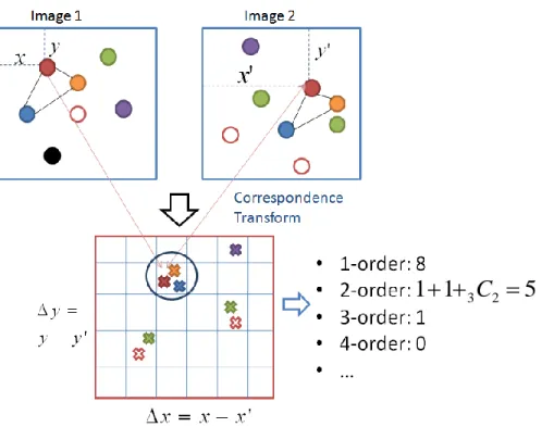
2.1 Illustration of the basic idea. Each circle in the top two images corresponds to a visual word (local feature). Different colors rep-resent different words. Two images are transformed to the off-set space (bottom image) in order to find the co-occurrence of high order features. Each cross in the offset space is created by a pair of same words (same color) form the two input images. The main idea is that when n points have the same location in the offset space, we have a particular co-occurringnorder feature. 4

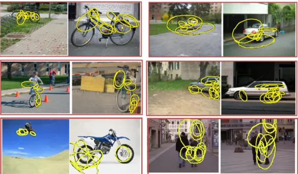
2.2 The images on the left show the matched High-Order Features

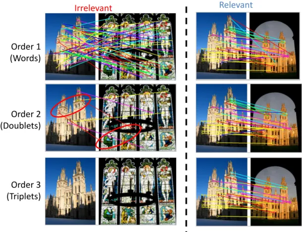
(HOF)of different orders for two irrelevant images, while the im-ages on the right show the matches for two relevant imim-ages (im-ages of the same object). The top row shows the matched visual words, which also correspond to the 1st order features, and the second and third rows show the 2nd order (doublets), and the 3rd order (triplets) features respectively. With the visual words, we have many matches for both images of different objects (left) and images of the same object (right). On the contrary, with the HOFs, we have much fewer matches for different objects than the same object. . . 6 2.3 Illustration of the algorithm for finding co-occurrences of

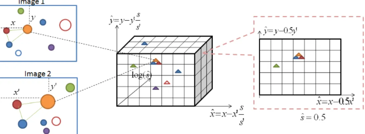
scale-invariant high order features. Each circle in the images is a local patch. The different colors represents different visual word as-signments. The size of the circle represents the scale of the patch. A triangle corresponds to a vote generated by a pair of patches. 13

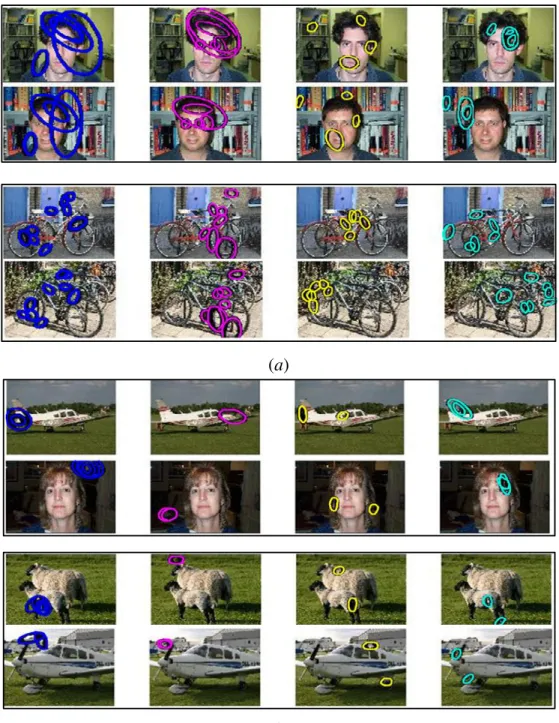
2.4 Example co-occurring HOFs. For each pair of images, we show

the HOF of the four largest order features being detected (from left to right). Different color represents different co-occurring features. At the top (a), the two images are from the same cate-gory. At the bottom (b), images are from different categories. We can find larger order features for images from the same category. 15 2.5 Example scale invariant HOF detected with our algorithm. For

each pair of images, we show the co-occurring HOF of the largest order detected. . . 16 3.1 Kernel Matrix of the training images for different order features.

From the left to right are 1st, 2nd, 3rd, 5th, 7th, 10th order kernel matrices. Training images are arranged in the categories of face,

(15)

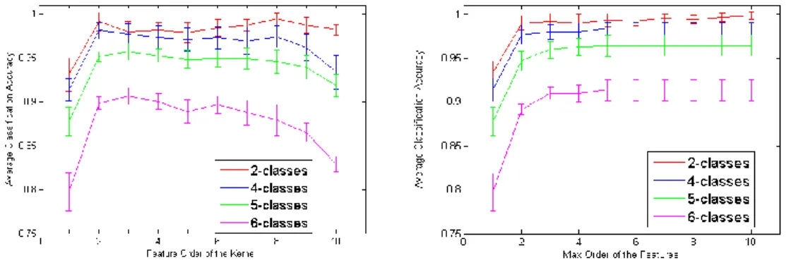
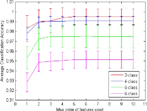
3.2 Object categorization performance with KNN (k=3). We show the average classification accuracy for classification task with 2, 4, 5, and 6 classes. Thexaxis is the feature ordern. The left figure shows the accuracy only using the nth order kernel. The right figure shows the accuracy using the summation of the kernels from 1 ton. . . 24 3.3 Object categorization performance with SVM. We use sum of the

individual kernels. . . 25 3.4 Categorization accuracies with vocabulary size 50. We show the

results for 6 class classification. . . 26

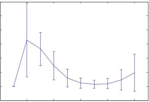
3.5 Learned weights for HOF kernel of different orders. We show

the average and standard deviation over the learned weights of all categories. . . 29

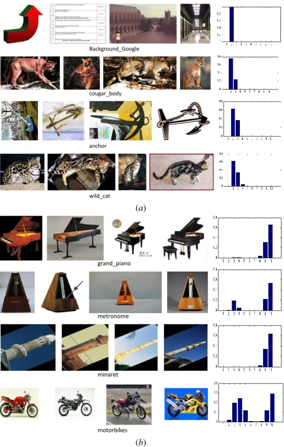
3.6 Learned weights of HOF kernels of different orders. We show

example categories that have lowest weights (a) and highest weights (b) for the higher (10th) orders. For each example cat-egory, example images and the learned weights for orders 1 to 10 are shown. . . 33 3.7 Average Accuracies when different step sizes are used for

quan-tizing the offset space. 15 images per category are used for training. 34 3.8 Average Accuracies of different methods when different number

of images per category are used for training. . . 35 4.1 The illustration of algorithms for calculating the scores of local

patches. The circles are the local patches. Different color repre-sents different word assignments. . . 42 4.2 The performances achieved by using the linear SVM method and

by the structured SVM method, both with bag-of-words features. 45 4.3 The performances achieved by features at different orders. The

black line is achieved by combining all four order features. The rest are achieved by using a single order feature. All the results are achieved from the structure SVM method. . . 47 4.4 Example detections. The green rectangles are the ground truth

bounding boxes, and the red ones are the predicted bounding boxes by our algorithm. . . 48 5.1 Inverted file structure and the illustration for updating the scores

of images with this structure. Green numbers are the offsets of word jand the word occurrences in the database, which are cal-culated online using the location of j. . . 55 5.2 Illustration of the min-hash method with HOF. . . 58 5.3 The effect of parameter changes on Oxford 5K dataset: mean

av-erage precisions with HOF of different orders. 1st order corre-sponds to the BoW model. . . 62

(16)

5.4 The precision-recall curve for example queries on the Oxford 5K dataset. (a) is for queryall souls 1, and (b) is forradcliffe camera 3. 65 5.5 The mean average precision of Oxford 5K dataset combined with

Flicker 1M images as distractors. . . 66

6.1 An example co-occurring spatio-temporal (ST) HOF of two

video sequences. The left images show space-time locations of the local features in each video. Red points indicate the fea-tures composing the co-occurring phrase. The right images show the frames (sampled at rate 5, frame index is shown) composing the phrase. Red circles indicate the local features composing the phrase. The ST-HOF captures the causality relationships among body parts from different individuals of a long time span for the same activity “push”. . . 70 6.2 3D correspondence transform. Circles represent local features,

and colors represent word assignments. A co-occurring ST-HOF of order 4 is shown. . . 74 6.3 Illustration of the incremental kernel computing algorithm. The

support vectors (selected training videos)S and their coefficients

α(second column) are obtained during training, while the offset spaces for each support vector (third column) need to be com-puted online during testing. The right most image shows the enlarged offset space between the video segmentVtand support vectorS1. . . 75

6.4 Hospital Surveillance Dataset. (a) ROC curve for all patients. (b) The AUC score for each patient. . . 81 6.5 (a) Accuracies for each category of the YouTube action dataset.

Average accuracies for BoW and ST-HOF for 63.7% and 72.9%, respectively. (b) Confusion matrix using ST-HOF. . . 87 6.6 Confusion Matrices on the UT interaction dataset (Set 1). . . 88 6.7 Example scenarios we aim to recognize from videos of the MPR

group dataset. . . 88 6.8 (a) The predicted probabilities (vertical) of various events at each

frame index (horizontal) for a test video. (b) Comparison of area under curve (AUC) scores for each event category on the whole test dataset. We compare the rule based method [10], BoW [139], and ST-HOF. Note that the rules forfightingare not defined in [10]. 89

(17)

7.1 Comparison of the object-based image segmentation results us-ing our methods and previous works. (b) 4-neighbor grid CRF [105] (c) RobustPn_{model plus object co-occurrence statistics [58]} (d) Our method with a fully connected CRF, which captures both long-range color contrasts and the object spatial relationships in addition to their global co-occurrences. Our method preserves the object contours without pre-segmentation and is able to place thefaceat the right place even if its unary probabilities are small. The result with our method is obtained in less than 3 seconds. . . 92 7.2 The illustration of the inference algorithm. The top row shows

the initial µi(xi) obtained from the unary terms. The second row shows the spatial relationships of different categories with “Face“ (to save space, we show them in smaller images). The third row illustrates the messages sent to “Face“ νi(xi,xj) . The bottom row shows the updatedµi(xi)after normalization. . . 100 7.3 The illustration for computing the frequency that the pixels

la-beled with “grass“ and “cow“ appear at different relative po-sitions (d px,d py). The rightmost image shows the resulting (d px,d py) space, which can be obtained with a cross-correlation from the ground truth of the two categories. . . 105 7.4 Analysis on the synthetic data where no unary cues are used.

The rightmost image on the top row shows the relative spatial distribution of each pair of categories. The middle and bottom rows show the performance of our method with and without color contrast term in the edge potentials respectively. The left-most images of these two rows plot the changes of the objective values in the QP relaxation at each iteration. The rest images show the changes of the predicted labels as we perform iterative updates. . . 107 7.5 Average running time (seconds) per iteration for max-product

belief propagation and the proposed method for a CRF defined over 213x320 pixels with edges over different neighborhood size. 108 7.6 Qualitative results on the Sowerby dataset when only absolute or

relative locations are learned during training. From left to right, we show the test image, grid CRF with random unary poten-tial, grid CRF with learned location potentials, proposed method with random unary potential, and the ground truth. . . 110 7.7 Results on the MSRC dataset with different CRFs . . . 112

(18)

CHAPTER 1

INTRODUCTION

In most vision techniques, images and videos are represented with local com-ponents, which capture the local appearances, such as edges, texture, and color, or local movements. The global shapes or contexts are modeled using the spa-tial information of the local components. Modeling the spaspa-tial information is challenging. On the one hand, we must encode enough spatial information in order to achieve enough precision of the vision tasks. For example, object recog-nition requires enough shape information to discriminate different object cate-gories. On the other hand, the shape information we encoded should be flexible enough to overcome the large intra-category variations, such as location or scale changes. Moreover, the resulting system should be computationally efficient enough.

This thesis is focusing on efficient algorithms that model rich spatial infor-mation of the local components. Existing methods on this problem usually suf-fer one or more of the following problems: 1) they extensively increase the com-putational cost by including more spatial information; 2) the spatial information is variant to pose changes, therefore, the methods require the objects in the im-ages aligned or require evaluating sub-windows in imim-ages; 3) the methods only encode weak spatial information, such as the neighborhood of each local com-ponent, or only distances between pairs of local components. In this thesis, we propose a family of algorithms that model higher order and longer range spatial information among the local components with little sacrifice of the invariance and computational cost.

(19)

We have explored two main vision problems: 1) image representation and 2) pixel-level image labeling. The main goal of the first problem is to obtain a nu-merical representation of the whole image so as to perform the tasks like object recognition/detection and image retrieval. Applications for pixel-level image labeling, such as image segmentation, tries to predict a label for every pixel in-stead of the whole image. For both problems, we have proposed algorithms that incorporate richer spatial information with much more efficiency comparing to prior work.

We propose our main algorithm for encoding spatial information to the whole image representation in Chapter 2, and its three variations for three appli-cations: object recognition in Chapter 3, object detection in Chapter 4 and image retrieval in Chapter 5. In Chapter 6, we extend this algorithm to the representa-tion of videos by adding a temporal dimension. Then, we present the algorithm that incorporates spatial information for the pixel-level image labeling problem and its application in Chapter 7. Finally, we conclude our work and point to future work in Chapter 8.

(20)

CHAPTER 2

IMAGE REPRESENTATION: HIGH ORDER FEATURES

2.1

Introduction

Most recent vision techniques represent an image with local features. In terms of the global geometry information, the Bag of words (BoW) representation [17] takes one extreme. It discards all spatial information of the local features. Due to its computational efficiency and intra-category invariance, BoW has been the most popular representation for many vision applications, such as object recog-nition, object detection and image retrieval. However, since it lacks the spatial modeling, the discrimination power is limited.

To incorporate spatial information to the BoW representation, one type of technique uses mutual geometry relationship between the local words [63, 74, 96, 118, 129, 133, 140]. Higher Order Features (HOFs) are constructed with a spe-cific number of local words, together with their spatial layout. Following the definition from [74], we call the local features 1st order features, and features with two, three, nwords, 2nd, 3rd andnth _{order features. The main advantage} of this type of methods is the invariance to translation or scale changes. How-ever, as the order increases, the dimension of the feature vector will increase exponentially to the order, and immediately reach an intractable amount. For example, when the vocabulary size is4000and the image space is modeled with a20×20grid, the dimension of 2nd order feature vector would be more than 1 billion, and as large as1019 _{for the 3rd order. To reduce the feature dimension,}

previous works only use up to 3rd order features [74, 118, 133, 140]. Moreover, the HOFs are usually created with local words in a short range with weak

(21)

ge-5

1



₃

C

₂



Figure 2.1: Illustration of the basic idea. Each circle in the top two images corresponds to a visual word (local feature). Different colors represent different words. Two images are transformed to the offset space (bottom image) in order to find the co-occurrence of high order features. Each cross in the offset space is cre-ated by a pair of same words (same color) form the two input images. The main idea is that whennpoints have the same lo-cation in the offset space, we have a particular co-occurringn order feature.

ometry, such as the co-existences in the same image or neighboring informa-tion [63, 96, 111, 129, 133, 140], and thus ignore long range interacinforma-tions.

We propose an efficient algorithm which is capable of handling unbounded (one toinfinite) order features with rich geometry. The main idea is illustrated in Figure 2.1. In order to find the co-occurring HOFs between two images, we transform the local features to the offset space. A vote is created in the offset space for each same word pair in the two images. The location in the offset space is the relative location of the two words. After transforming to the offset

(22)

space,nvotes at the same location indicatenwords of the same mutual spatial layout in the two images, which correspond to a co-occurringnthorder feature. After the transformation, it would be quite easy to find the co-occurring HOFs, which is intractable in the original image space. Figure 7.1 illustrates the benefit of matching two images using the HOFs detected with our algorithm. With the visual words, we have many matches for both images of different objects (left) and images of the same object (right). On the contrary, with the HOFs, we have much fewer matches for different objects than the same object. When we increase the order to 3, we cannot find any matches for the two irrelevant images.

We can further prove that the number of co-occurring nth _{order features} equals to the inner product of the histograms ofnth_{order features of the two} im-ages. In standard procedure for computing the inner product, the system first computes the histograms, and then the distance between the histograms. Both of these steps require exponentially large computation. In comparison, our al-gorithm computes one to infinite order features with the same computational complexity as BoW.

For different vision applications, we can easily integrate the efficiently com-puted inner-product of HOF histograms to other state-of-arts methods to re-place original BoW representation. In object recognition (Chapter 3) and object detection (Chapter 4), we use the inner product as a kernel for the SVM. For object detection (Chapter 4), we also propose an efficient sub-window search algorithm for the HOFs to avoid evaluating every sub-windows in an image. For the large-scale image retrieval application (Chapter 5), we use the proposed algorithm to calculate the cosine similarity of the high order feature vectors of

(23)

Order 1

(Words)

Order 2

(Doublets)

Order 3

(Triplets)

Irrelevant

Relevant

Figure 2.2: The images on the left show the matchedHigh-Order Features (HOF)of different orders for two irrelevant images, while the images on the right show the matches for two relevant images (images of the same object). The top row shows the matched

visual words, which also correspond to the 1st order features, and the second and third rows show the 2nd order (doublets), and the 3rd order (triplets) features respectively. With the vi-sual words, we have many matches for both images of differ-ent objects (left) and images of the same object (right). On the contrary, with the HOFs, we have much fewer matches for dif-ferent objects than the same object.

the query image and images in the database. To avoid comparing the query with every image in the database, we integrate the proposed algorithm with the inverted files structure, and remain the computational cost similar to that of the BoW method for image retrieval. For activity recognition from videos

(24)

(Chapter 6), we further extend the algorithm from 2D to 3D by adding the tem-poral domain to capture both the spatial and temtem-poral relationships of the local movements.

2.2

Related Work

2.2.1

BoW and Beyond

One of the most popularly used technique in computer vision is the Bag-of-Words (BoW) representation of images [17, 83, 88, 106, 137]. Local features are detected at interest regions or sampled densely from the images, and then are assigned to visual words that are learned usually with K-means. The BoW dis-cards any geometry information of the local features and represents an image as a histogram of the visual words. Due to its computational simplicity and robustness to transformation variances, BoW has gain great success in many applications, such as object recognition, detection and image retrieval.

Recent work that improve BoW are mainly on: 1) encoding methods that create a better word representation for each local feature, such as sparse coding [130] or locality sensitive coding [120]; 2) pooling techniques that aggregate the words/codes in an image to a vector representation, such as average pooling (same as histogram) and max pooling [120]. Geometric lp-norm pooling [28] and receptive fields pooling [45] learns the features that are most important for classification to select from images; 3) approaches that encode geometry and shape information to BoW by modeling the locations of the words. This paper is along the third line of work. Our approach is general enough to be easily

(25)

combined with advances from the first two types of work.

2.2.2

Spatial Modeling

We will review the prior works that incorporate the spatial information into the BoW representation in details for different applications in Chapter 3, 4, 5, and 6. Generally speaking, there are mainly four types of methods: 1) Spatial Pyramid Matching (SPM) [21, 65, 125, 130] based methods incorporate rigid spatial infor-mation by quantizing the image space into grid regions and thus are not trans-lation or scale invariant; 2) star shaped models [25,66,81,132], which models the location distribution of the words relative to the center of the object, and thus re-quire object bounding boxes for the training images. 3) Constellation model [29] constructs a graph with latent nodes representing a fixed number of parts, and is translation and scale invariant. However, this type of models is usually com-putational expensive; 4) High Order Feature based models [63, 74, 96, 102, 118] construct composite features that capture the mutual geometrical relationship between the local words. Our work belongs to this type. Comparing to prior work, our algorithm is more efficient so as to compute much higher (up to infi-nite) order features and encode much richer geometry.

(26)

2.3

Main Algorithm

2.3.1

Image Representation

An image I is represented as a collection of local patches, I = {p1, ...,pm}. Each patch is represented with its visual word assignmentw, region size sand loca-tionx,y. pi = (wi,si,xi,yi).

2.3.2

High-Order Feature

We define the high order features (HOF) with one word 1st order features, and features with two, three, n words, 2nd, 3rd and nth _{order features. Different} relative spatial distribution among thenvisual words yields differentnth_order features. Figure 2.1 shows example occurrences of the same 3rd order feature in two images. An image will be represented as the histogram defined with the HOFs. The dimension of this histogram can be extremely long even when n = 2while a large vocabulary is used. Therefore, it is impractical to create the histograms directly and perform the computation.

2.3.3

Correspondence Transform

For the explanation simplicity, we first only consider the translation invariance for the HOF. The main idea of the algorithm is that if two HOF co-occur in two images, they must be a translation from one image to the other. Thus, we can simplify the task of counting co-occurrence ofnthorder features in two images

(27)

to counting the constant shiftnvisual word pairs in the two images. However doing this directly on the image space would be still too much. In order to facilitate this process, we first transform the feature points in two images to the offset space. The idea is illustrated in Figure 2.1. We call this “Correspondence Transform”. For each pair of same words in the two images, we calculate their offset(4x,4y), which is the location of the word in imageI1minus that in image

I2. Then a vote is generated in the offset space at(4x,4y). If there are multiple

correspondences for the same word, we create multiple votes, as the green and red words. In the offset space,nvotes locating at the same position corresponds to a co-occurringnth order feature. Thus, to count the number of co-occurring nth

order features in the two images, we can simply count the number ofnvotes at the same location in the offset space. In the example of figure 2.1, the number of co-occurring 2nd order features is1+1+3₂; while the number for 3rd order feature is1, since we only have 1 position with 3 votes. And for all n > 3, the number is0since we do not have larger than 3 votes at the same location. We summarize the algorithm as in Algorithm 1.

(28)

Algorithm 1: Compute the number of co-occurring HOFs

Input: Two images represented with visual words: I1= {vi},I2= {vj}

Output: Number of co-occurring nth order features, Kn(I1,I2), for all n =

1,2, ...,∞ Algorithm:

1. Perform correspondence-transform:

(a) For each pair of same words in the two images (vi ∈ I1,vj ∈ I2) , compute

their offset(∆x= xi−xj,∆y=yi−yj).

(b) Create a vote in the offset space at(∆x,∆y)

2. In the quantized offset space, for each bin that hasN(N ≥n)votes: IncrementKn(I1,I2)withN choosen,

_N n . Kn(I1,I2)= Kn(I1,I2)+ _N n .

2.3.4

Relationship with HOF Histogram

We analyze the relationship between the co-occurring HOFs of two images and their HOF histograms. Thenth order histogram of an image I is a vector Φ(I)

with the fn coordinate as the number of occurrences of feature fn. The inner-product of the HOF histograms of two images can be computed as follows.

< Φ(I1),Φ(I2)> (2.1) = X fn <Φfn(I1),Φfn(I2)> (2.2) = X fn X un=fn,un∈I1 1× X un=fn,un∈I2 1 (2.3) = X fn X un=fn,un∈I1 X un=fn,un∈I2 1. (2.4)

whereun= fn,un∈I1indicates thatunis an occurrence of feature fnin imageI1.

(29)

to the total number of co-occurringnthorder features. We example the usage of this inner product for different applications in the later sections. Notice that if we directly compute the histograms and then compute the inner-product, the computation time would be|Σ|n_{× |}_X_|n−1_|_Y_|n−1_{, where}_|Σ_|_{is the visual word}

vocab-ulary size and X,Y are the X and Y axes of the image space. While using the proposed algorithm, the running time is the linear to the number of same word pairs. Moreover, with this computation, we have calculated all order (one to

infinite) features.

2.3.5

More Invariance

Adding more invariance is as easy as adding more dimension to the offset space. Taking scale invariance as example, as illustrated in figure 2.3, we add a scale dimension to the offset space. Let(xi,yi)denote the position of wordi, andsi de-note the size of the region used to create this word. For each pair of same words iandi0in the two images, we create a vote at( ˆx,yˆ,sˆ)= (xi− _ssi0

ix 0 i,yi− si s0 iy 0 i,log( si s0 i)).

In the 3D offset space, if we have n votes at the same location, we have a co-occurringnth

order feature with both translation and scale invariance. In figure 2.3, at scale difference sˆ = 1/2, we have a co-occurring 3rd order feature. Rota-tion invariance can be similarly incorporated.

2.3.6

Computation Time

Let Pdenote the number of same word pairs of two images. It takesO(P)time to calculate the offset space with Algorithm 1. In the worst case (all features in

(30)

Figure 2.3: Illustration of the algorithm for finding co-occurrences of scale-invariant high order features. Each circle in the images is a lo-cal patch. The different colors represents different visual word assignments. The size of the circle represents the scale of the patch. A triangle corresponds to a vote generated by a pair of patches.

the two images are assigned to the same word), we haveP=O(M2₎_{same word}

pairs, where M is the number of features per image. However, in practice, the number of same word pairs is linear to M. Especially with a large vocabulary size,Pis usually even smaller than M. Therefore, in practice we only needO(M)

time to compute all (1 toinfinite) order features, which is the same complexity as BoW.

2.4

Example Visualization

Figure 2.4 shows the example co-occurring HOF in two images detected with our algorithm. Figure 2.5 shows the example scale-invariant HOF detected in two images.

(31)

2.5

Different Applications

For different vision applications, we make different usage of the inner product of HOF histograms computed efficiently with the proposed algorithm. In the following chapters, we will present four example usages: object recognition, object detection, image retrieval, and activity recognition from videos.

(32)

(a)

(b)

Figure 2.4: Example co-occurring HOFs. For each pair of images, we show the HOF of the four largest order features being detected (from left to right). Different color represents different co-occurring features. At the top (a), the two images are from the same cat-egory. At the bottom (b), images are from different categories. We can find larger order features for images from the same cat-egory.

(33)

Figure 2.5: Example scale invariant HOF detected with our algorithm. For each pair of images, we show the co-occurring HOF of the largest order detected.

(34)

CHAPTER 3

HOF FOR OBJECT RECOGNITION

The goal of the object recognition task is to determine whether an object is in-cluded in an image. This is essentially a classification task, which classifies an image into a pre-defined object category. Bag-of-Words (BoW) model has gain great success in this task [17, 137].

3.1

Related Work

For the task of object recognition, the most widely used method for encoding ge-ometry information to BoW is the Spatial Pyramid Matching (SPM) [11,65]. SPM incorporates rigid spatial information by quantizing the image space into grid regions, and has achieved the state-of-the-art performance when combined with advanced coding and pooling techniques [28, 45, 120], on datasets like Caltech-101 [93] where objects are centered and aligned in images. However it lacks in-variance to translation or scale differences of the objects. Another type is the star shaped models [81], which model the location distribution of the words relative to the center of the object, and thus require object bounding boxes for the train-ing images. Constellation model [29] represents the objects with a fixed number of parts and captures the spatial layout of the parts with a joint Gaussian, and can be translation and scale invariant. However, this type of models is computa-tionally expensive in that it requires searching an exponentially large number of hypothesis which give different part assignments to the features. Graph based models [22, 67] find a geometrically consistent matching between features from two images by optimizing a graph, which has a node for each pair of local

(35)

fea-tures, and thus can be quite large.

Another extension for improving the BoW representation is to model the mutual geometry relationship among the words [63, 74, 96, 118]. Our work be-longs to this type. Comparing to prior work, our algorithm is more efficient so as to compute much higher (up to infinite) order features and encode richer geometry.

3.2

HOF as SVM Kernel

3.2.1

HOF Kernel

We use the inner-product of HOF histograms as the kernel for the Support Vec-tor Machine (SVM), which is equivalent to performing classification with SVM in the HOF space rather than the word space. To define a metric as a SVM kernel, it is known that the Mercer’s condition (positive semi-definite) must be satisfied so as to guarantee that the learning of the SVM results in a global op-timal. Since we define the kernel as an inner product, it satisfies the Mercers condition from its definition.

The co-occurrence can be efficiently computed with the algorithm proposed in previous Section. Specifically, the kernel Kn(I1,I2)of thenth order features of

imagesI1,I2is defined as follows.

Kn(I1,I2)=<Φn(I1),Φn(I2)> . (3.1)

(36)

normal-ize the feature vector. Thus the normalnormal-ized kernelKˆn(I1,I2)is as follows, ˆ Kn(I1,I2) = < Φn(I1) ||Φn(I1)|| , Φn(I2) ||Φn(I2)|| > (3.2) = Kn(I1,I2) √ Kn(I1,I2)Kn(I2,I2) . (3.3)

Our final kernel is a weighted sum of allKˆn(I1,I2)’s.

K(I1,I2)=

∞

X n=1

wnKˆn(I1,I2). (3.4)

One way to set the weightswn is usingµ1−nwith µa pre-defined value of(0,1). Asµgets closer to zeros, we put more weights to the higher order features.

With this kernel, the decision score of the SVM for a testing imageS(I)would be S(I) = X i yiαiK(I,si) (3.5) = X i yiαi X n wnKˆn(I,si), (3.6)

where si are the support vectors (training images) of the SVM, yi ∈ {+1,−1}are their corresponding class labels, and αi denote the learned coefficients of the support vectors.

3.2.2

Combine HOF Kernels with MKL

We can further refine the kernel K(I1,I2)(Equ. 3.4) by learning the weights wn with training images. The intuition is that different objects may have different weights for different orders. Objects with rigid shapes, likefaces, should have higher weights on higher orders, while objects with less rigid shapes, likecat, should have higher weights on lower orders.

(37)

The Multiple Kernel Learning (MKL) techniques [2, 115] would be suitable for this purpose. In previous work for object recognition, MKL has been applied for combining kernels computed from different types of features, such as color, texture and shape [33, 116]. We use it for combining kernel matrix of different order features.

The main idea of MKL is to formulate the SVM so that it learns the coefficient

αi (Equ. 3.6) and the weights for different kernel matrixwnat the same time. We use the MKL technique proposed in [115] and the code provided by the authors. HOF kernels of orders 1 to 10 are combined, and a SVM with a different set of weights is learned for each class.

3.2.3

Coding Local Features

The HOF histogram in the algorithms explained above assumes that each local feature is hard quantized to a single visual word. Many papers have shown that using soft quantization improves the performance [120, 130]. In soft quantiza-tion, each local feature is assigned to a set of words with non-zero codes com-puted using various coding schemes, such as Sparse Coding [130] and Locality-constrained Linear Coding [120]. We show that our HOF algorithm can be easily adapted for this case.

Now since the local words are associated with weights (codes), we define the weight for a HOF as the summation of the weights of the words composing it: c(f) = P

wi∈f ci, where ci denotes the code for word wi. Thus, the dot

prod-uct of the vector representations of two images equals to the summation of the weights of the co-occurring HOF. Suppose an offset bin of two images has N

(38)

votes generated from words w1, ...,wN; the summation of the weights of HOFs of ordernin this bin can calculated as follows:

X f∈{w1,...,wN}n c(f)= N−1 n−1 ! N X i=1 ci. (3.7)

Therefore, to associate the HOF with weights, we simply modify the equation in the 2nd step of Algorithm 1 with

Kn(I1,I2)= Kn(I1,I2)+ N−1 n−1 ! N X i=1 ci. (3.8)

3.3

Experiments

In this section, we evaluate our algorithm for the object recognition task with the public datasets: Caltech-101 [93] and Graz-01, Graz-02 [88]. We would like to verify that using Higher Order Features (HOFs) effectively encodes geom-etry information to the Bag-of-Words (BoW) model and improves the perfor-mance. Moreover, we compare favorably with other approaches for modeling the geometry information. For each dataset, we extract local features with the detectors and descriptors that achieve the state-of-the-art results on the corre-sponding dataset. These experiments also show the flexibility of our approach on different types of local features.

Practical Issue: Due to the large dimension of the feature space, images will have extremely sparse representations in the HOF feature space. This also leads to the fact that the kernel value of the same image will be much larger than that of two distinct images. Thus, our kernel matrix will be nearly diagonal, espe-cially for higher order. This is called diagonal dominance in machine learning, and is proved to be a problem when the kernel matrix is applied to learning

(39)

algorithms such as SVM. Many methods have been proposed to overcome this problem [37]. We applied the negative diagonal shift method, which is to sub-tract a constant from the diagonal of the kernel matrix. Although it is possible make the kernel matrix not positive semi-definite any more, it has shown to gain good performance in practice.

3.3.1

Caltech-6

First, on a subset of the Caltech-101 dataset, we analyze some important factors of our approach. We use images of six object categories from the Caltech 101 dataset: faces, motorbikes, airplanes, rear cars, watches, ketches. We apply Harris-Laplacian interest point detector [83] and SIFT descriptors [77]. We report clas-sification results for two classes (faces and motorbikes), four classes (faces, mo-torbikes, airplanes, and rear cars), five classes (4 classes + watches), and six classes.

Kernel Matrix

Figure 3.1 shows the kernel matrix of the training data with five classes for different order features. As the order increases, the matrix gets darker (values are smaller) at the off-diagonal places, and thus is more discriminative among different categories. However, the diagonal places (same category image pairs) also get darker for some categories, such as airplane and rear car, with higher orders (7 or 10). This is due to the fact that few co-occurring higher order fea-tures are detected for some image pairs in the same category when the category includes more variance in object shapes. Faces and Motorbikes are two objects with the most consistent structures.

(40)

takes time to pair the same words in two images and calculate the offsets of the pairs (step 1 and 2), where is the number of pairs created. To cluster the pairs with the same offsets and update the kernel needs time. In the worst case (only one visual word occurs in each image), we have pairs. However, in practice we can only form pairs linear to . Especially with a large codebook size, the number of pairs we form can be even smaller than . Moreover, after running one time of the algorithm, we have already calculated all order kernels. Therefore, in practice we only need time to calculate the kernels of all order features, which is the same complexity with calculating a kernel with bag of words model.

3.Experiments

We evaluate the proposed kernel for object categorization task. We use several public datasets: Caltech-101, MSRC dataset [18], and Graz-01 dataset. For all the datasets, we use the whole images (No bounding box) for both training and testing, which we believe is an advantage for our algorithm, since the high order kernels support partially matching similarities. Figure 9 gives some example co-occurring high order features found by the proposed algorithms.

3.1.Implementation Issues

For all the datasets, we apply Harris-Laplacian interest point detector [15] and SIFT detector [13] to each gray scale image to get the local features. The local features are further clustered with K means algorithm to obtain the visual words. We apply the proposed kernels to K nearest neighbor and Support Vector Machine for the classification task. For the implementation of SVM, we used the public library Libsvm [2]. For stableness, we do not consider scaling and rotation in these experiments.

Due to the large dimension of the feature space, images will have extremely sparse representations in the feature space. This also leads to the fact that the kernel based self-similarity of an image will be much larger than the similarity between two distinct images. Thus, our kernel matrix will be nearly diagonal, especially for large order. This is called diagonal dominance in machine learning, and is proved to be a problem when the kernel matrix is applied

to learning algorithms such as SVM. Many methods have been proposed to overcome this problem [6]. We applied the negative diagonal shift method, which is to subtract a constant from the diagonal of the kernel matrix. Although it is possible make the kernel matrix not positive semi-definite any more, it has shown to gain good performance in practice.

3.2.Effect of High Order Features

We use six object categories from the Caltech 101 dataset: {faces, motorbikes, airplanes, rear cars, watches, ketches}. This dataset has previously been used for unsupervised object category detection [7], while we use it in a supervised way. The goal of this experiment is to explore the change of the classification performance and computational time as we increase the order of the features. For all the six categories, there are more than 100 images per category, and reliable interest point can be detected. The task is to classify an image to one of the six categories. For the experiments, we randomly choose 50 images per category for training and 50 other images for testing. We repeat this 10 times and present the average results. We set the dictionary size as 500. We report the results of classification for two classes (faces and motorbikes), four classes (faces, motorbikes, airplanes, and rear cars), five classes (4 classes + watches), and six classes. We first use the step size 16 for image quantization in the experiments. For SVM, we use the one-vs-one scheme implemented in Libsvm for the multi-class classification.

Kernel Matrix

Figure 4 shows the kernel matrix of the training data with five classes for different order features. As the order increases, the matrix gets sparser and sparser, thus more discriminative among different categories. However, the inner class similarity matrix also gets sparser for some categories, such as airplane and rear car, with large orders (7 or 10). This is due to the fact that few co-occurring large order features are detected for some image pairs in the same category when the category includes more variance in object structure, scale, or rotation. Faces and Motorbikes are two objects with the most consistent structures.

Individual vs. Cumulative

We show the classification results with K Nearest Neighbor classifier ( 3 in Figure 5. We use the

Figure 4: Kernel Matrix of the training data for different Order features. From the left to right are 1st_{, 2}nd_{, 3}rd_{, 5}th_{, 7}th_{, 10}th_{order kernel}

matrices. Training data is arranged in the categories of ‘face’, ‘airplane’, ‘rear car’, ‘motorbike’, and ‘watches’. As the order increases, the matrix gets sparser and sparser.

Figure 3.1: Kernel Matrix of the training images for different order fea-tures. From the left to right are 1st, 2nd, 3rd, 5th, 7th, 10th order kernel matrices. Training images are arranged in the categories offace,airplane,rear car,motorbike, andwatches.

Individual vs. Cumulative

We show the classification results with K Nearest Neighbor classifier (k=3) in Figure 3.2. We use the normalized kernel as the similarity function for KNN. We present both the results of individual kernelsKnwith only thenthorder features, and the results of the sum of kernels from 1st to nth _{order individual kernels.} We show the performance until 10th _{order since most images do not have} co-occurring features whose order are larger than 10. We found that for both indi-vidual and cumulative kernels, we gain significant improvement from 1st order (bag of words) to 2nd order features, which proves that modeling geometry in-formation helps a lot. For the individual case, we get best performance with8th order kernel for 2 class classification task, 2nd for 4 class, and 3rd for both 5 and 6 class. The accuracy dropping is mainly because as the order increases, fewer images will have co-occurring features as we have seen in the kernel matrix (Figure 3.1). For the cumulative case, the accuracy generally keeps increasing as we increase the order (may stop growing at some order). We found that even if individually the accuracy drops for the higher order kernels, they may still con-tribute to the performance when we add them together. This is not surprising given the fact that higher order features are more discriminative. We reach best performance when the maximum order is 10 for 2 class, 5 for 4, 5, and 6 class

(41)

Figure 3.2: Object categorization performance with KNN (k=3). We show the average classification accuracy for classification task with 2, 4, 5, and 6 classes. The x axis is the feature order n. The left figure shows the accuracy only using thenth _{order kernel.} The right figure shows the accuracy using the summation of the kernels from 1 ton.

classification tasks.

Using as Kernel for SVM

We apply the kernel to the SVM. Figure 3.3 shows the results for the sum of the individual kernels. The accuracy with SVM is better than that with KNN for all the orders. We can still see the performance increase as we increase the order.

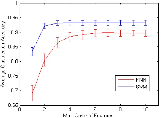
Vocabulary Size

The experiments till now are using a vocabulary size 500. We now decrease the vocabulary size to 50. Figure 3.4 shows the classification performance when using KNN and SVM. In this case, the individual visual words would be more ambiguous, which results in low accuracies when using low order features. Es-pecially for KNN, the accuracy is under 70% when using bag of words model. However, for both KNN and SVM, as we increase the order of the features, we got the performance quite close to that when we use 500 visual words. This

(42)

Figure 3.3: Object categorization performance with SVM. We use sum of the individual kernels.

shows that even if the local features are not discriminative itself, by increasing the orders, we can create discriminative high order features.

Running Time

We run our experiments on a single CPU of a 2.26G Quad-Core Intel Xeon server with 12G memory. Computing the kernel values for a pair of images takes 0.2ms with a Matlab+C implementation.

3.3.2

Caltech-101

The whole Caltech-101 dataset [93] contains 9144 images of 101 object cate-gories. Each category includes 31 to 800 images. Following previous work

(43)

Figure 3.4: Categorization accuracies with vocabulary size 50. We show the results for 6 class classification.

[93,115,120], we train the SVM classifiers by randomly selecting 5,10,15,20,25,30 images per class and test with no more than 50 images. Experiments are re-peated 5 times and the average accuracies are reported.

In this experiment, we use the same feature detector and descriptor as [120]: local patches of size16×16are extracted densely at every 6 pixels on the image and represented with the Histogram of Oriented Gradient (HOG) descriptor. The same coding scheme (Locality-constrained Linear Coding) [120] is applied to create the visual words and their codes. We use a vocabulary size of 1024 learned with Kmeans, and encode each local feature to its 2 nearest neighbor words. Previous work [120, 130] have shown that a max-pooling step on the codes of the descriptors improves the performance. For our implementation, we also max-pool the sub-regions of a2×2grid, and apply our HOF algorithm

(44)

on the pooled local features. We found that this step is important whendense

features are used, where many nearby features are assigned to the same word, and thus create unreliable HOFs.

Word Encoding

Table 3.1 compares our approach with Bag-of-Words (BoW), Spatial Pyra-mid Matching (SPM) L2 (level 1-2), and SPM-L3 (level 1-3). The same pipeline as [120] is used for SPM. For SPM, level 2 and 3 uses 2× 2 and 4× 4 grid re-spectively. We show the average accuracies and standard deviations over all 102 categories when 15 training images are used. Performance using different word encoding methods are reported. For words obtained with hard vector quantization (VQ), we use χ2 _{kernel for both BoW and SPM, which performs}

better than a linear kernel. While for words obtained with Locality-constrained Linear Coding (LLC) [120], we use linear kernels for both BoW and SPM, since

χ2_{kernel performs worse than the linear one in this case. Our methods use the}

proposed HOF kernel in both cases.

The table shows that HOF outperforms other methods in both average ac-curacy and standard deviation no matter which coding method is used. More-over, HOF can be successfully combined with LLC coding to further improve the classification accuracies.

Combine HOF Kernels

Table 3.1 also shows that using the learned weights for combining differ-ent order kernels (HOF-learned) improves the performance of the method that manually sets fixed weights for all categories.

(45)

Table 3.1: Average accuracies on Caltech 101 dataset. Classifiers are trained with 15 images per class. For different methods, we show the performance using different word encoding method: hard vector quantization (VQ) and Locality-constrained Linear Coding [120]. We compare our method (HOF) with BoW, Spa-tial Pyramid Matching (SPM) of level 1 and 2 (2×2), and SPM of level 1 to 3 (4×4). HOF-learned use the learned weights for combining different order kernels.

BoW SPM - L2 SPM -L3 HOF HOF-learned

VQ 44.26±_2.24 _51.2±_1.12 _57.09±_0.89 _61.87±_0.33 62.94±0.35

LLC 37.18±_1.95 _52.2±_0.68 _64.55±_0.56 _67.17±_0.36 68.28±0.35

Figure 3.5 shows the learned weights of HOF kernel of different orders aver-aged over all categories. For the multiple kernel learning, we usel1norm for the weights of different orders, which favors sparsity of the weights. Interestingly, all categories give zero weight for the first order kernel (BoW). The reason is be-cause all object categories in Caltech-101 are in some particular shape (although some are more rigid), and thus combining the orderless word based kernel with other HOF kernels do not help. Second order feature gets the highest weight in general. Many categories give zero weights to 6-8th order features, which is probably because the information of these order features can be captured by other orders.

In figure 3.6, we present the learned weights of HOF kernels (order 1 to 10) for categories that have lowest weights (left) and highest weights (right) for the

10thorder. As we expected, the objects, which are more rigid in shape and more consistent in appearance, get higher weights for the higher orders. For lower orders, the opposite trend is shown.

(46)

0 2 4 6 8 10 −0.1 0 0.1 0.2 0.3 0.4 0.5 0.6 Order Weight

Figure 3.5: Learned weights for HOF kernel of different orders. We show the average and standard deviation over the learned weights of all categories.

Offset Space Quantization

In our algorithm for computing the co-occurring HOFs of two images (Al-gorithm 1), we consider any N votes that fall in the same bin of the quantized offset space as a co-occurring Nth order feature. Figure 3.7 shows the average accuracies when different step sizes are used for the quantization. Intuitively, smaller step size will work better for objects of more rigid shape. Our final ker-nel combines the kerker-nels computed with step size 5,10,15,20,30, and achieved the better result.

Comparison

Figure 3.8 compares our approach with BoW and SPM under various num-ber of training images per category. Exactly the same local features and the

(47)

same coding method (LLC) are used for these methods. Therefore, the figure proves that our HOF based approach outperforms the performance of BoW by incorporating geometry information among the local words. Moreover, our ap-proach also outperforms SPM which is a popular method for encoding spatial information to BoW.

Finally, we compare the performance of our approach with other recent work that achieve the state-of-the-art results on the Caltech-101 dataset in table 3.2. Methods cited in the top rows of the table use similar local features (dense HOG/SIFT) and similar coding methods as us, but different ways for encoding the geometry information. ScSPM [130] and LLC+SPM [120] uses Spatial Pyra-mid Matching (SPM); RLDA [47] and Receptive Field [45] improves SPM by im-proved algorithms for creating the bins of the image space. The bottom rows of the table present the performance of other methods that either use different type of features (SPM [64], NBNN [6], Deconv. Net [135], LP-B (MKL) [33]), different pooling method (Deconv. Net [135]), or different classifiers (NBNN [6], De-conv. Net [135]). In particular, LP-B (MKL) [33] uses Multiple Kernel Learning to combine many different types of features, such as texture, color, shape, and self-similarity. GLP [28] proposes a different pooling (feature selection) method other than max-pooling and achieves the best result on this dataset. The im-provement of these methods is orthogonal to ours, since our approach can be applied to any local features and can always be plugged in after the pooling step to capture the geometry relationship of the words remained.

(48)

Table 3.2: Average accuracy (%) comparison on Caltech-101. Top: methods that use the similar local features as ours. Bottom: other recent work that achieve good results on Caltech-101.

Training images 5 train 15 train 30 train

ScSPM [130] - 67 73.2 LLC+SPM [120] 51.15 65.43 73.44 RLDA [47] - - 73.7 Receptive Field [45] - - 75.3 Ours (HOF-learned) 55.14 68.28 77.23 SPM [64] - 56.4 64.6 NBNN [6] - 65 70.4 Deconv. Net [135] - - 71 GLP [28] 59.35 70.34 82.6 LP-B (MKL) [33] 54.2 70.4 77.7

3.3.3

Graz-01, Graz-02

The Graz-01, Graz-02 datasets [88] include objects of various scales. Objects in these datasets have large location and scale differences; therefore, methods that are not translation and scale invariant, such as Spatial Pyramid Matching, are not suitable. Figure 2.5 shows example images from the datasets. Follow-ing previous work [72] on these dataset, we use harris-hessian interest region detectors [82] and SIFT feature descriptor [77]. We build the vocabulary with K-means usingK = 500. Translation and scale invariance are considered during the experiments. We adopt the same training and testing split as in [88].

(49)

pre-Table 3.3: Equal Error Rate (%) on the Graz dataset

Dataset Class BoW [88] Pair [67] PDK [72] HOF

Graz01 Bicycle 86.5 84.0 95.0 96.0 Person 80.8 82.0 88.0 90.0 Graz02 Bike 77.8 92.0 86.7 88.0 Person 81.2 86.0 86.7 92.0 Car 70.5 n/a 74.7 80.3

vious works. We outperform other methods which use bag of words [88], and methods that encode geometry information with pair of words [67] [72] on most categories.

(50)

Background_Google cougar_body anchor wild_cat (a) grand_piano metronome minaret motorbikes (b)

Figure 3.6: Learned weights of HOF kernels of different orders. We show example categories that have lowest weights (a) and highest weights (b) for the higher (10th) orders. For each example

(51)

cat-60

62

64

66

68

70

5

10

15

20

30

combined

A

cc

u

ra

cy

Step_size

Figure 3.7: Average Accuracies when different step sizes are used for quantizing the offset space. 15 images per category are used for training.

(52)

20

30

40

50

60

70

80

0

5

10

15

20

25

30

BOW

SPM-L2

SPM-L3

HOF

HOF-learned

Figure 3.8: Average Accuracies of different methods when different num-ber of images per category are used for training.

(53)

CHAPTER 4

HOF FOR OBJECT DETECTION

The task of object detection not only recognizes whether an object is in an image, but also detects the location of the object. In this chapter, we introduce how to efficiently adopt the proposed HOF algorithm for this task.

A naive way to perform object detection with the HOFs is the sliding win-dow approach, which performs classification for every possible sub-winwin-dows in an image. Classification can be done in the same way as “object recognition” (Chapter 3) with the HOF kernel for the SVM. However, this method would require computing kernel values for a large number of sub-windows per im-age. We propose an efficient algorithm which obtains the decision scores for all sub-windows with only a single kernel calculation for the entire image.

Moreover, we present the method that integrates the HOF algorithm into the structured learning framework. Unlike the sliding window approach, which learns a binary classifier for the sub-windows in an image, the structured learn-ing can formulate the output of the classifier as the location of the object of interest. Thus the training of the classifier is directly optimizing the localization performance.

4.1

Related Work

The sliding window approach [9, 18, 25, 30] been widely used for object detec-tion. During training, a binary classifier which determines the presence of the object of interest in a sub-window is trained with a sample of positive and

(54)

neg-ative examples. During testing, the classifier is evaluated at every possible lo-cation and scale in a test image to localize the object in the image. Despite the effectiveness of the approach, one main disadvantage is that the training is not directly optimizing the detection performance.

Structured learning has been used to address the problem of the sliding win-dow approach [4, 5]. Rather than predicting a binary label, the classifier with structured learning is learned to predict a more structured output, which is the bounding box of the object for the object detection task. A bounding box is parameterized as the top, left, bottom and right coordinates of the box. Thus the output space of the object detection task can be represented with the four numbers. Thus, the classifier is trained to directly optimize the detection per-formance.

One important issue with structured learning is the efficiency for the infer-ence, since the size of the output space is quite large. To learn a structured classifier, we usually need to iteratively perform inference on the training data to find the negative examples. To efficiently find the optimal bounding box in an image, previous works use the branch and bound algorithm with the Bag of Words (BoW) representation [4, 59]. However, BoW representation does not model the shape of the object, and thus is not discriminative enough. We incor-porate the HOFs to the structured learning framework to improve the perfor-mance of BoW, and provide an efficient sub-window search algorithm when the HOFs are used.

(55)

4.2

Object Detection with HOF

4.2.1

Structured Learning Review

The outputs of a classifier learned with the structure learning [113] are not sim-ple binary labels, but instead have a more comsim-plex structure. This allows us to better model the relationship between different outputs within the output space. In order to formulate object detection as a problem of predicting struc-tured data, we follow the framework proposed in [4]. We briefly introduce the framework here.

In the context of object detection, the problem is defined as below: given a set of input images {x1,· · · ,xn} ⊂ X and their associated object annotations

{y1,· · · ,yn} ⊂ Y, we wish to learn a mapping f : X → Y with which we can automatically annotate unseen images. The output space consists of two parts: a label indicating whether an object is present, and a vector indicating the top, left, bottom, and right of the bounding box within the image: Y ≡ {(ω,t,l,b,r)|ω ∈ {+1,−1},(t,l,b,r) ∈ _R4_}_. _ω ₌ ₋₁_{indicates no object is present. So the coordinate}

vector (t,l,b,r)is ignored in this case. The mapping from X_to Y _{is learned in}

the structure learning framework [113] as f(x;ω)=arg max

y∈Y F(x,y;ω) (4.1)

where ω denotes a parameter vector and F(x,y;ω) is a discriminant function. We further assume F to be linear in some feature representation of inputs and outputsψ(x,y),

F(x,y;ω)=<w, ψ(x,y)> (4.2) The feature representationψ(x,y) will be defined in Section 2.3.2. To train the

(56)

discriminant function, F(x,y;ω), we use the structured SVM method proposed in [113] min ω,ξ 1 2kωk 2₊_C n X i=1 ξi (4.3) s.t. ξi ≥0,∀i (4.4) hω, ψ(xi,yi)i − hω, ψ(xi,y)i ≥∆(yi,y)−ξi,∀i,∀y∈ Y \yi (4.5) where ω= n X i=1 X y∈Y\yi αiy(ψ(xi,yi)−ψ(xi,y)) (4.6)

and ∆(yi,y) is a loss function chosen to reflect the quantity that measures how well the localization performs. In this work, the loss function∆(yi,y)is defined as Equation 4.7. ∆(yi,y)=            1− Area(yi∩y) Area(yi∪y) ifyiω =yω = 1 1−(1₂(yiωyω+1)) otherwise (4.7)

The loss function has the following properties: 1) it is equal to 1 when the labels of the bounding boxes disagree; 2) it is equal to 0 when the labels of the bound-ing boxes are both negative; 3) it is measured by the area overlap between the boxes when the labels of the bounding boxes are both positive.∆(yi,y)is 1 if the boxes are identical and 0 if they are disjoint.

The key problem for solving the generalized SVM learning is the large num-ber of margin constraints defined in Equation 4.5. Following the methods pro-posed in [113], we here use a cutting plane method to find a subset of active constraints that ensures a sufficiently accurate solution. It is equivalent bew-teen Equation 4.5 and

ξi ≥ max y∈Y\yi

(57)

In training, we iteratively repeat the following: 1) estimate ω using the fixed subsets of constraints; 2) add new constraints by finding y that maximize the right part of Equation 4.8. In testing, we findythat maximizes Equation 4.1.

4.2.2