A Kernel Partial Least Square Based Feature Selection Method

(1)

Accepted Manuscript

A Kernel Partial Least Square Based Feature Selection Method Upasana Talukdar, Shyamanta M Hazarika, John Q. Gan

PII: S0031-3203(18)30182-1

DOI: 10.1016/j.patcog.2018.05.012

Reference: PR 6556

To appear in: Pattern Recognition

Received date: 20 April 2017 Revised date: 23 April 2018 Accepted date: 13 May 2018

Please cite this article as: Upasana Talukdar, Shyamanta M Hazarika, John Q. Gan, A Ker-nel Partial Least Square Based Feature Selection Method, Pattern Recognition (2018), doi:

10.1016/j.patcog.2018.05.012

This is a PDF file of an unedited manuscript that has been accepted for publication. As a service to our customers we are providing this early version of the manuscript. The manuscript will undergo copyediting, typesetting, and review of the resulting proof before it is published in its final form. Please note that during the production process errors may be discovered which could affect the content, and all legal disclaimers that apply to the journal pertain.

(2)

ACCEPTED MANUSCRIPT

Highlights

• The paper proposes a Kernel Partial Least Square (KPLS) based Feature Selection Method aiming for easy computation and improving classification accuracy for high dimensional data.

• The proposed method makes use of KPLS regression coefficients to identify an optimal set of features, thus avoiding non-linear optimization.

• Experiments were carried out on seven real life datasets with four different classifiers: SVM, LDA, Random Forest and Na¨ıve Bayes.

• Experimental results highlight the advantage of the proposed method over several competing feature selection techniques.

(3)

ACCEPTED MANUSCRIPT

A Kernel Partial Least Square Based Feature Selection Method

Upasana Talukdara_{, Shyamanta M Hazarika}b_{, John Q. Gan}c

a_{Biomimetic & Cognitive Robotics Lab,Dept. of Computer Science & Engineering,Tezpur University, India} b_{Dept. of Mechanical Engineering, Indian Institute of Technology, Guwahati, India}

c _{School of Computer Science and Electronic Engineering, University of Essex, United Kingdom}

Abstract

Maximum relevance and minimum redundancy (mRMR) has been well recognised as one of the best feature selection methods. This paper proposes a Kernel Partial Least Square (KPLS) based mRMR method, aiming for easy computation and improving classification accuracy for high-dimensional data. Experiments with this approach have been conducted on seven real-life datasets of varied dimensionality and number of instances, with performance measured on four different classifiers: Naive Bayes, Linear Discriminant Analysis, Random Forest and Support Vector Machine. Experimental results have exhibited the advantage of the proposed method over several competing feature selection techniques.

Keywords: Feature Selection, Kernel Partial Least Square, Regression Coefficients, Relevance, Classification.

1. Introduction

In high-dimensional feature space, feature dimensionality reduction through selection of highly predictive features plays an indispensable role in pattern recognition. The aim of fea-ture selection is to identify the most informative feafea-tures that ”optimally characterizes” the class [1]. In literature, feature selection algorithms are broadly classified into three main cat-egories: filter, wrapper and embedded. For wrapper methods, the optimal characterization

∗_{Corresponding author}

Email addresses: [email protected](Upasana Talukdar),[email protected]

(4)

ACCEPTED MANUSCRIPT

condition signifies the maximal classification accuracy or minimal classification error with respect to a particular classifier, whereas for filter methods they emphasise the dependency of the features on the target class [1]. Embedded methods differ from filter and wrapper because of the interaction of feature selection and learning process. In such methods feature selection and learning can not be separated [2]. Filter methods are fast, since they do not incorporate learning [2]. One of the most widely used tactics in filter methods is maximal relevance, i.e., selecting features with highest relevance with the target class [1].

Relevance between features and the target class has been characterized in terms of dif-ferent statistical measures such as information gain [3], mutual information [1, 4, 5, 6, 7, 8], correlation [9, 10] and regression coefficients [11, 12, 13, 14]. Population based heuristic search methods such as particle swarm optimization [15, 16], genetic algorithms [16, 17, 18], ant colony optimization [19, 20, 21], simulated annealing [22], rough set [23] and fuzzy rough set [24] have been used. The amalgamation of simulated annealing and genetic algorithm has also found its application in selecting optimal feature subset [25]. Gargari et al. [26] proposed an optimal feature selection method using Branch and Bound. Selection of opti-mal features has also been attained using Support Vector Machines (SVM) [27, 28, 29] and recursive feature elimination method [30]. Besides, unsupervised methods have also been used [8, 31, 32, 33].

Regression coefficients have attained quite popularity in identifying the relevance between the features and the class [34]. Regression coefficients reflect the rate of change of one variable with respect to other thus reflecting the relevance between the two. Partial Least Square (PLS) has widely been used in this context [11, 12, 13, 14]. The advantage of PLS over other regression methods like least square is that it maps the predictor and the response variable onto some uncorrelated components called latent vectors and then applies regression onto these components. Hence it is suitable for high-dimensional data. The commonly used metrics to identify an optimal set of features based on PLS are Selectivity Ratio (SR)

(5)

ACCEPTED MANUSCRIPT

[11, 12, 35], Significance of Multivariate Correlation (SMC)[12, 35] and Variable Importance Projection (VIP) [12, 35]. However, PLS is useful for feature selection in linear systems only. Rosipal et al [36] proposed a non-linear PLS technique called Kernel Partial Least Square (KPLS) for dealing with non-linear systems. Besides KPLS, different non-linear variants of PLS have been proposed. KPLS is found to perform better than PLS as well as its other non-linear variants [37, 38]. This study employs KPLS to select an optimal set of features. Its efficacy has been compared with different non-linear methods used for selecting features. The main advantage of KPLS lies in the fact that it avoids nonlinear optimization by using kernel functions that correspond to the inner product in the feature space. It is a fast and effective method for non-linear systems [39]. KPLS maps the data onto latent vectors and then applies regression onto these components, which makes it suitable for high-dimensional data as well. Thus the method is applicable for both small and large data. The aim of this paper is to exploit the advantage of KPLS for feature selection in non-linear systems through the use of the KPLS regression coefficients to compute the depen-dency between a feature and its target class. As an alternative to mutual information in mRMR [1], this paper proposes a KPLS regression coefficients based feature selection method that identifies an optimal set of features by exploiting maximum feature-class relevance and minimum feature-feature redundancy in terms of KPLS based relevance scores.

The proposed method will be evaluated in terms of classification accuracy of four classi-fiers on seven datasets including UCI datasets, gene expression dataset and BCI Competi-tion dataset of varied dimensionality and number of instances. Four well known classifiers: Support Vector Machine (SVM) [40], Random Forest [41], Naive Bayes [42] and Linear Discriminant Analysis (LDA) [43] have been tested. The effectiveness of the method has been compared with four filter methods: MI-mRMR [1], KPLS based Selectivity Ratio (SR) [11, 12, 35], Coefficient of Determination (R), Significance Multivariate Correlation (SMC) [12, 35], two embedded methods: Lasso [44] and Elastic Net [45] and Deep Learning [46] in

(6)

ACCEPTED MANUSCRIPT

terms of 10-fold cross-validation classification accuracy.

The rest of the paper is organized as follows. The concept of KPLS and the proposed method are introduced in Section 2. Section 3 presents the experimental results while Section 4 discusses the findings. Finally, Section 5 concludes the paper.

2. KPLS-mR and KPLS-mRMR for feature subset selection

KPLS method models a non-linear relationship between a set of output data Y and a set of input data X. It maps the original input variables to some higher-dimensional function spaceFand then applies the PLS algorithm onto the transformed data. Fcan be of high and even infinite dimension, in which PLS regression is computationally expensive [35]. KPLS solves this using the kernel trick: the kernel function evaluates an inner product between two vectors in F : k(xi,xj)=φ(xi)Tφ(xj), ∀xixj ∈X [35]. Different kernel functions are available

such as sigmoid kernel, polynomial kernel or radial basis (Gaussian) kernel [39]. Among these kernels, radial basis kernel is most common [39]. Detailed algorithms and equations for KPLS can be found in [36, 39].

In this paper KPLS regression coefficient is used to determine the relevance of a feature with its target class. Based on the regression coefficient obtained for a feature and its class (or between two features), a unique weight is assigned to each feature, which reflects the relevance of the feature with its class (or with another feature). This is termed asRel Score

(Definition 1).

Definition 1. Relevance Score (Rel Score) : It is a number based on regression coeffi-cients of class labels w.r.t. features which tells how much relevant a feature f is w.r.t. its class c. This gives the feature-class relevance score (Rel Score(f_|c)). Similarly, relevance score computed based on the regression coefficients of a selected feature f1 w.r.t. non-selected features tells how much relevant a non-selected feature f2 is w.r.t. f1. This gives the feature-feature relevance score (Rel Score(f2|f1)).

(7)

ACCEPTED MANUSCRIPT

Maximum relevance (mR) of a feature with its target class is obtained by searching the features based on theRel Score. The feature with the highest Rel Score is the most relevant feature while the feature with the lowest Rel Score is the least relevant.

Based onRel Score(f|c), wheref is a feature and c is its target class, maximum relevance (mR) can be defined as in Equation 1

mR=max

i (Rel Score(fi | c)) (1)

It is likely that features selected based on their relevance with the class might have high redundancy, i.e., the relevance among these features might be large [1]. When two features are highly relevant with each other, the respective class-discriminative power will not differ much if one of them is discarded [1]. Hence, redundant features can be removed. This criterion of selecting least redundant feature is minimum redundancy (M R) [1].

LetF be the set of all features,F’ be the set of selected features. Minimum redundancy based on Rel Score(fi | fj ) where fj ∈ F’; fi ∈ S;S=F-F’ is defined as in Equation 2

M R =min

i (Rel Score(fi | fj )) (2)

The criterion that combines Equations (1) and (2) is called “maximal relevance and minimum redundancy” (mRMR) [1]. The mRMR feature set is identified by optimizing the conditions in equations (1) and (2) simultaneously. Combining the two equations into a single criterion functionR can be achieved by optimization of both conditions as follows:

R=max(mR−(γ×M R)) (3)

(8)

ACCEPTED MANUSCRIPT

howRperforms for different values of γ which is checked in two different ranges [0.1,1] and [1,10]. The first range starts withγ=0.1, since with γ=0, R would behave similarly to mR (Equation 1). This range of γ values provides more weightage to mR . It ends with γ=1 providing equal weightage to mR and MR. The second range starts withγ=1 and ends with

γ=10. This range provides more weightage to MR.

In practice, suppose we have a set F with n features and a set of selected features F’

withm-1 features. The task is to select the mth feature from the set S=F-F’. In that case, redundancy of each featurefi ∈S christened as Rfi is evaluated as in Equation 4.

Rfi = 1 m₋1 X fj∈F0 [Rel Score(fi|fj)] (4)

The search method then selects the mth feature from S by optimizing the following condition in whichR is rewritten as follows:

R=max

fi∈S

[mR−γ×Rfi] (5)

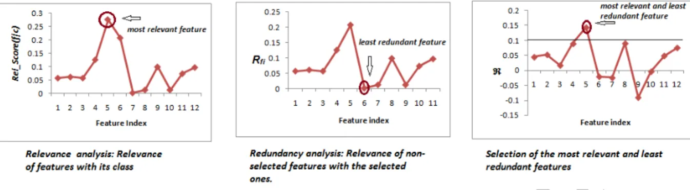
Fig. 1 portrays the relevance analysis of the features. The leftmost graph shows the feature-class relevance analysis, i.e., Rel Score(f_|c), the middle graph shows the feature-feature redundancy analysis (Equation 4) and the rightmost graph illustrates Equation 5. In order to find out whether using R described in Equation 5 is more effective than using mR described in Equation 1 for the proposed KPLS-based feature selection, two algorithms named KPLS-mR and KPLS-mRMR are investigated by experiments in this paper. They are described by Algorithm 1 and Algorithm 2, respectively.

Both KPLS-mR and KPLS-mRMR depend on two major modules, namely KPLS and Compute RS.

(9)

ACCEPTED MANUSCRIPT

Figure 1: Illustration of relevance as well as redundancy analysis of features. The circled point in the leftmost graph is the most relevant feature as selected by mR (Equation 1) while the circled point in the rightmost graph is the maximum relevant and minimum redundant feature selected byR(Equation 5). The black horizontal bar in the rightmost graph acts as the threhold so as to select the feature with maximum value ofR.

Algorithm 1: KPLS-mR

Input: F=set of n features and N samples, Y=set of class labels

Output: F’=an optimal subset of k features R=KPLS(F,Y);

Rel Score(f|c) = Compute RS(F,R);

[weight,FeatureRank]=descend(Rel Score(f|c));//Rel Score(f|c) in descending order

foreach i _≤ k do

F’(i)=FeatureRank(i); i++;

end

//FeatureRank comprises of the features with most relevant in the first position and least relevant in the last.

function Compute RS(F,R) w =F−1_R;

w=w2_;

Rd=sum(R);

dor=Rdw;

Rel Score =sqrt(dor/Rd);

returnRel Score

(10)

ACCEPTED MANUSCRIPT

Algorithm 2: KPLS-mRMR

Input: F=set of n features and N samples, Y=set of class labels, γ,count=1

Output: F’=an optimal subset of k features R=KPLS(F,Y);

Rel Score(f_|c) = Compute RS(F,R);

[weight,FeatureRank]=descend(Rel Score(f|c));//Rel Score in descending order F’(1)=FeatureRank(1);// Select feature with max. feature-class Rel Score F=F-F’(1);

while count ≤ (k-1) do

ffR=0;

foreach feature fj ∈ F’ do

R=KPLS(F,fj);

Rel Score(f|fj) = Compute RS(F,R);

ffR=ffR +Rel Score(f_|fj);

end

Rf=average ffR;

foreach feature fi ∈ F do

R=Rel Score(fi|c)−(γ × Rfi) forfi ;

end [weight,FeatureRank]=descend(R); F’=F’ ∪ FeatureRank(1); f1=FeatureRank(1); F=F-f1; count=count + 1; end function Compute RS(F,R) w =(F−1_R)2_; Rd=sum(R); dor=Rdw; return(sqrt(dor/Rd)); end function

(11)

ACCEPTED MANUSCRIPT

coefficients between them using KPLS algorithm. KPLS first makes use of kernels that map ’a’ to some high-dimensional function space. It then computes uncorrelated latent vectors (components) on the transformed data using SIMPLS algorithm [47]. A least square regression is then performed on the subset of the extracted latent vectors. The size of the subset of latent vectors is set by 10-fold cross-validation. The module computes regression coefficients between features and class as well as between two features.

2. Compute RS(a,b): For a given feature set’a’ and regression coefficients’b’, Compute RS returns theRel Score between a feature and its class or a feature with another feature.

3. Experimental Results

Experiments were carried out on a workstation with 12 GB RAM, Intel(G) Xeon pro-cessor and 64 bit windows 7 operating system. The proposed methods were implemented using MATLAB R2015a.

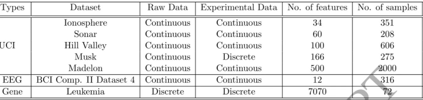
For our experiments, seven different real-life datasets of varied dimensionality and num-ber of instances have been used. The detailed descriptions of the datasets are in Table 1. Note that the Musk data from UCI-ML repository has been discretized for experimental purpose using equal width binning method.

The proposed algorithms KPLS-mR and KPLS-mRMR have been evaluated in terms of 10-fold cross-validation classification accuracy with four well-known classifiers: SVM, Random Forest, LDA and Naive Bayes. The proposed methods were compared with four existing filter based feature selection algorithms: MI-mRMR, SR, R and SMC, two embedded feature selection methods: Lasso and Elastic Net and Deep Learning.

Our approach to select an optimal set of features consists of two key steps:

1. KPLS model selection: The samples of the datasets were split into equal sized training and testing partitions to compute the KPLS scores. The number of KPLS components

(12)

ACCEPTED MANUSCRIPT

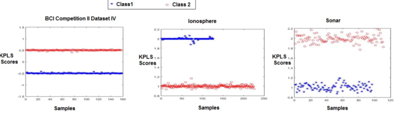
Figure 2: KPLS Scores for optimal number of KPLS components depicting perfect separation of the classes

were checked in the range of 1 to 6. The optimal number of KPLS components was determined on the KPLS scores by 10-fold cross-validation classification accuracy for radial basis kernel. KPLS takes as input two matrices X and Y. The Y matrix is a vector of class labels. The X is a n_×m matrix with n being the number of samples and m being the number of features. KPLS regression coefficients are computed on training data. KPLS scores are then estimated in testing by projecting the testing data on the KPLS regression coefficients found in training. The optimal number of KPLS components was then determined on the KPLS scores by 10-fold cross-validation classification accuracy for radial basis kernel. Fig. 2 portrays the KPLS scores of different classes for three datasets: BCI Competition II Dataset 4, Ionosphere and Sonar datasets. All the three datasets consist of two classes. The figure shows that KPLS scores for the optimal number of KPLS components are distinctively different for the two classes depicting that it perfectly separates two classes.

2. Use of the selected model for feature selection: The KPLS model selected as described above was then applied to select the optimal set of features for each dataset. The method involves four basic steps. 1) computation of KPLS regression coefficients using SIMPLS algorithm, 2) computation of Rel Score(f|c) andRel Score(f2|f1) based on regression coefficients for each feature, 3) computation of R and 4) selection of

(13)

ACCEPTED MANUSCRIPT

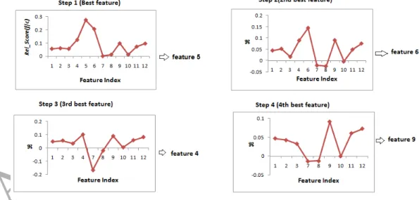
features based on R. For the KPLS-mRMR method, the optimalγ value was obtained by searching it in two different ranges : [0,1] where γ increases by 0.1 and [1,10] where γ increases by 1. The optimal γ value was then set by 10-fold cross-validation classification accuracy. The optimal gamma value obtained for different datasets with different classifiers are shown in Table 2. The R computed based on the optimal gamma value is taken as the final measure for identifying the set of optimal features. Fig. 3 portrays each step of selecting a feature from the set of non-selected features based on R. The figure shows the selection of the best four features of the BCI Competition II Dataset 4. The first feature with maximum Rel Score(f_|c) is feature 5, hence feature 5 is selected first and is removed from the set of non-selected features. Next, feature 6 has the highest R and hence is selected. The process is repeated till the desired number of features are selected. Note that both SR and R give the same set of optimal features for each dataset. Hence, while comparing the performances of different feature selection methods, SR and R have not been interpreted separately.

Figure 3: Selection of features using KPLS-mRMR

(14)

ACCEPTED MANUSCRIPT

Table 1: Dataset Description

Types Dataset Raw Data Experimental Data No. of features No. of samples

UCI

Ionosphere Continuous Continuous 34 351

Sonar Continuous Continuous 60 208

Hill Valley Continuous Continuous 100 606

Musk Continuous Discrete 166 275

Madelon Continuous Continuous 500 2000

EEG BCI Comp. II Dataset 4 Continuous Continuous 12 316

Gene Leukemia Discrete Discrete 7070 72

Table 2: Optimal gamma values obtained for different datasets with different classifiers

Dataset LDA Naive Bayes Random Forest SVM

Ionosphere 0.53 0.53 0.1 0.1

Sonar 7 5 10 10

Hill valley 0.2 0.1 0.2 0.2

Madelon 0.1 0.1 0.1 0.1

Musk 0.1 0.1 0.1 0.2

BCI Comp. IV Dataset 2 0.4 0.4 0.1 0.1

Leukemia 0.53 0.2 0.2 0.53

MI-mRMR we have referred Peng’s implementation 1_{. For the implementation of the two}

embedded methods: Lasso and elastic net, we have referred Karl’s webpage2 _{while for the}

implementation of Deep Learning, we have used simple convolutional neural network3_.

3.1. Comparison with other filter methods

The cardinality of the selected feature subset for the filter methods for different datasets varies according to the dimension of the datasets. BCI Competition II Dataset 4 consists of 12 features and the maximum number of selected features was set to 4. Maximum number of selected features for Hill Valley consisting of 100 features was set to 20 whereas for Sonar dataset consisting of 60 features was set to 15. For all other datasets, the maximum number of selected features was set to 10. To compare the results, one way ANOVA followed by Scheffe’s posthoc test [48] was conducted. The results are shown in tables. Each table

1_{http://penglab.janelia.org/proj/mRMR/} 2_{http://www.imm.dtu.dk/projects/spasm/}

3

(15)

ACCEPTED MANUSCRIPT

shows the comparison of KPLS-mR with MI-mRMR, SR and R and SMC followed by the comparison of KPLS-mRMR with the four aforesaid methods. The comparison is made based on p-values. A p-value less than 0.05 is considered to indicate significantly better performance by KPLS-mR or KPLS-mRMR than the above four methods (indicated by

X) while a p-value greater than 0.05 is considered to be insignificant or worse performance (indicated by ×). Furthermore, the size of the optimal feature set identified by different methods using different classifiers are also tabulated. In all such tables classifiers are listed in the first column, feature selection methods, size of the optimal set of selected features and 10-fold cross-validation accuracy with the selected feature subset are given in the 2nd, 3rd and 4th column respectively.

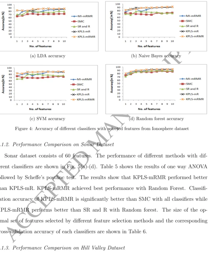
3.1.1. Performance Comparison on Ionosphere Dataset

Ionosphere dataset consists of 34 features. The performance of different methods with different classifiers are shown in Fig. 4(a)-(d). The results of one way ANOVA followed by Scheffe’s posthoc test are in Table 3.

Table 3: Statistical Test on Ionosphere Dataset

Method 1 Method 2 LDA Naive Bayes Random Forest SVM KPLS-mR

MI-mRMR 1.55e−5_X _0.0028_X _0.32828_× _0.000215_X

SMC 5.12e−19 _X _7.48e−24_X _3.38e−6_X _4.28e−21 _X

SR and R 9.97e−11 _X _1.59e−21_X _0.0002_X _2.3e−15_X

KPLS-mRMR

MI-mRMR 1.43e−6_X _0.008_X _0.4536_× _0.000156_X

SMC 9.37e−20 _X _4.81e−23_X _7.52e−6_X _3.44e−21 _X

SR and R 1.04e−11 X 1.04e−20X 0.00043X 1.75e−15 X

KPLS-mR and KPLS-mRMR achieved significantly better classification performance than all the other methods with LDA, Naive Bayes and SVM classifiers. The size of the optimal set of features selected by each feature selection method and the corresponding cross-validation accuracy of each classifier are shown in Table 4.

(16)

ACCEPTED MANUSCRIPT

(a) LDA accuracy (b) Naive Bayes accuracy

(c) SVM accuracy (d) Random forest accuracy Figure 4: Accuracy of different classifiers with selected features from Ionosphere dataset

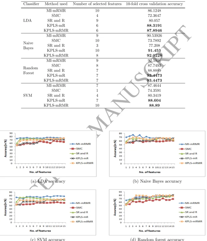
3.1.2. Performance Comparison on Sonar Dataset

Sonar dataset consists of 60 features. The performance of different methods with dif-ferent classifiers are shown in Fig. 5(a)-(d). Table 5 shows the results of one way ANOVA followed by Scheffe’s posthoc test. The results show that KPLS-mRMR performed better than KPLS-mR. KPLS-mRMR achieved best performance with Random Forest. Classifi-cation accuracy of KPLS-mRMR is significantly better than SMC with all classifiers while KPLS-mRMR performs better than SR and R with Random forest. The size of the op-timal set of features selected by different feature selection methods and the corresponding cross-validation accuracy of each classifiers are shown in Table 6.

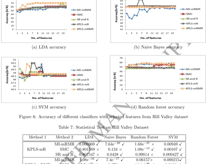
3.1.3. Performance Comparison on Hill Valley Dataset

Hill Valley dataset consists of 100 features. The performance of different methods with different classifiers are shown in Fig. 6(a)-(d).The results of one way ANOVA followed by

(17)

ACCEPTED MANUSCRIPT

Table 4: Performance Comparison on Ionosphere Dataset

Classifier Method used Number of selected features 10-fold cross validation accuracy

LDA MI-mRMR 10 86.1248 SMC 4 72.3647 SR and R 9 80.057 KPLS-mR 6 88.3191 KPLS-mRMR 6 87.8946 Naive Bayes MI-mRMR 9 90.53926 SMC 10 73.7892 SR and R 3 77.208 KPLS-mR 10 91.453 KPLS-mRMR 8 92.0228 Random Forest MI-mRMR 9 92.5926 SMC 8 87.7493 SR and R 7 88.8889 KPLS-mR 7 93.4473 KPLS-mRMR 7 93.4473 SVM MI-mRMR 7 87.4644 SMC 1 74.3591 SR and R 4 80.3419 KPLS-mR 7 88.604 KPLS-mRMR 10 88.89

(c) SVM accuracy (d) Random forest accuracy Figure 5: Accuracy of different classifiers with selected features from Sonar dataset

(18)

ACCEPTED MANUSCRIPT

Table 5: Statistical Test on Sonar Dataset

MI-mRMR 6.83e−18_× _3.94e−18 _× _0.841512_× _2.25e−29_×

SMC 0.001046X 4.58e−6 _X _4.83e−10_X _2.74e−10 _X

SR and R 1.01e−10_× _0.0009_× _0.464_× _5.14e−16_×

KPLS-mRMR

MI-mRMR 1.18e−7_× _7.87e−7 _× _0.977_× _1.04e₋₂₂_×

SMC 1.08e−13X 2.23e−17X 2.56e−13X 1.09e−18 X SR and R 0.097358_× 0.4388_× 0.010X 1.86e−7_×

Table 6: Performance Comparison on Sonar Dataset

Classifier Method used No. of selected features 10-fold cross validation accuracy

LDA MI-mRMR 10 77.4038 SMC 12 67.3077 SR and R 14 75 KPLS-mR 10 71.6346 KPLS-mRMR 15 75.4808 Naive Bayes MI-mRMR 3 75.9615 SMC 4 60.53769 SR and R 11 67.788 KPLS-mR 10 67.3077 KPLS-mRMR 4 69.7115 Random Forest MI-mRMR 12 78.8462 SMC 12 70.6731 SR and R 15 78.8462 KPLS-mR 15 80.7692 KPLS-mRMR 7 80.7692 SVM MI-mRMR 15 78.81 SMC 13 60.0962 SR and R 4 74.5192 KPLS-mR 14 67.7885 KPLS-mRMR 8 69.2308

(19)

ACCEPTED MANUSCRIPT

(c) SVM accuracy (d) Random forest accuracy Figure 6: Accuracy of different classifiers with selected features from Hill Valley dataset

Table 7: Statistical Test on Hill Valley Dataset

MI-mRMR 0.000369X 7.64e−28 _X _1.68e−37_× _0.00949_X

SMC 0.801589× 0.134× 1.08e−14X 0.00107X SR and R 0.807547_× 0.0428X 0.99814_× 0.009427X KPLS-mRMR

MI-mRMR 1.08e−34_X _7.4e−17_X _0.06157_× _0.000215_X

SMC 5.5e−24X 0.079× 4.14e−26X 0.0118X SR and R 5.19e−24_X _0.0275_× _1.99e−42_X _0.3477_×

Scheffe’s posthoc test are shown in Table 7. KPLS-mRMR performed best with LDA, SVM and Random Forest classifier. With Naive Bayes both KPLS-mR and KPLS-mRMR achieved better performance than MI-mRMR. The number of selected features and the corresponding cross-validation accuracy for each classifier are shown in Table 8. It can be seen that KPLS-mRMR achieved the best classification accuracy using the selected feature set, as compared to others with all the classifiers. KPLS-mR performs worst with Random Forest

(20)

ACCEPTED MANUSCRIPT

Table 8: Performance Comparison on Hill Valley Dataset

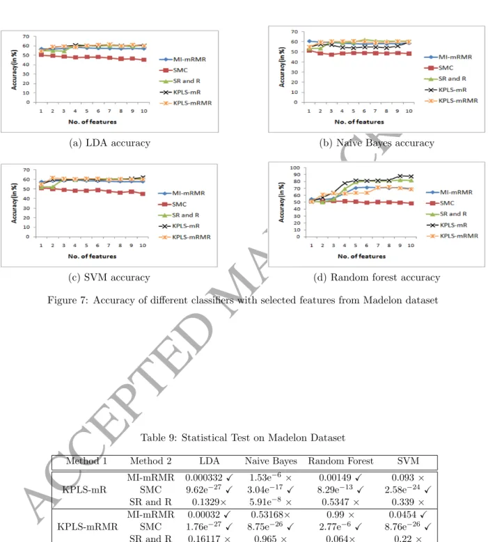
3.1.4. Performance Comparison on Madelon Dataset

Madelon Dataset is a highly non linear dataset consisting of 500 features. The results in terms of classification accuracy for different classifiers are shown in Fig. 7(a)-(d). The results of one way ANOVA followed by Scheffe’s posthoc test are shown in Table 9. The results show that with LDA both KPLS-mR and KPLS-mRMR performed significantly better than MI-mRMR and SMC. With Naive Bayes KPLS-mRMR gave insignificantly improved performance over MI-mRMR, SR and R; while with SVM, KPLS-mRMR gave significantly better performance than MI-mRMR and SMC. The number of selected features and the corresponding cross-validation accuracy for each classifier are shown in Table 10. It is observed that KPLS-mRMR achieved best classification accuracy with LDA and SVM with the set of selected features than all the other methods.

3.1.5. Performance Comparison on Musk Dataset

Musk Dataset version 2 has 168 features. For the analysis, the last 166 features have been used. The results in terms of classification accuracy for different classifiers are shown

(21)

ACCEPTED MANUSCRIPT

(c) SVM accuracy (d) Random forest accuracy

Figure 7: Accuracy of different classifiers with selected features from Madelon dataset

Table 9: Statistical Test on Madelon Dataset

MI-mRMR 0.000332 X 1.53e−6 _× _0.00149_X _0.093_×

SMC 9.62e−27 X 3.04e−17X 8.29e−13 X 2.58e−24 X SR and R 0.1329_× 5.91e−8 _× _0.5347_× _0.339_×

KPLS-mRMR

MI-mRMR 0.00032X 0.53168_× 0.99_× 0.0454X SMC 1.76e−27 _X _8.75e−26_X _2.77e−6 _X _8.76e−26 _X

(22)

ACCEPTED MANUSCRIPT

Table 10: Performance Comparison on Madelon Dataset

LDA MI-mRMR 4 58.7 SMC 1 50.3 SR and R 4 61.05 KPLS-mR 7 61.55 KPLS-mRMR 7 61.6 Naive Bayes MI-mRMR 1 60.6 SMC 1 51.35 SR and R 7 62.1 KPLS-mR 10 59.8 KPLS-mRMR 5 60.75 Random Forest MI-mRMR 6 71.6 SMC 4 51.4 SR and R 10 75.15 KPLS-mR 9 88.1 KPLS-mRMR 8 72 SVM MI-mRMR 4 59.6 SMC 1 50.8 SR and R 4 60.85 KPLS-mR 10 61.1 KPLS-mRMR 2 61.55

Table 11: Statistical Test on Musk Dataset

MI-mRMR 0.99298× 0.4924× 0.686× 0.5372×

SMC 0.978_× 0.9934_× 0.999_× 0.9978_× SR and R 1.02e−18 _X _1.21e−17_X _0.011_X _2.54e−17 _X

KPLS-mRMR

MI-mRMR 0.967_× 0.5327_× 0.72_× 0.73_×

SMC 0.991× 0.982× 0.99× 0.97×

SR and R 1.44e−18 _X _8.96e−18_X _0.009_X _1.33e−18 _X

in Fig. 8(a)-(d). One way ANOVA followed by Scheffe’s posthoc test was conducted and the results in terms of cross-validation accuracy of different classifier are shown in Table 11. With all the four classifiers, KPLS-mR and KPLS-mRMR performed significantly better than SR and R methods whilst their performance was similar to MI-mRMR and SMC. The number of selected features and the corresponding cross-validation classification accuracies are shown in Table 12. The results show that KPLS-mRMR produced best performance in terms of classification accuracy with Random Forest using the selected features .

(23)

ACCEPTED MANUSCRIPT

Figure 8: Accuracy of different classifiers with selected features from Musk dataset Table 12: Performance Comparison on Musk Dataset

3.1.6. Performance Comparison on BCI Competition II Dataset 4

This dataset consists of only one subject and two classes: left hand and right hand movement. Common Spatial Pattern (CSP) features are extracted from three frequency

(24)

ACCEPTED MANUSCRIPT

Figure 9: Accuracy of different classifiers with selected features from BCI Competition II Dataset IV

bands: alpha, theta and beta and thus the feature vector consists of 12 features, 4 features from each band. The maximum number of selected features was set to 4. The results in terms of classification accuracy of different classifiers with the selected features are shown in Fig. 9(a)-(d). One way ANOVA followed by Scheffe’s posthoc test was conducted and the results are shown in Table 13. The results show that with LDA, SVM and Naive Bayes classifiers KPLS-mR and KPLS-mRMR performed significantly better than SMC, SR and R but performed similarly to MI-mRMR. The number of features and corresponding cross-validation accuracies are shown in Table 14. It conveys that the performance of KPLS-mRMR is the best with all the classifiers.

3.1.7. Performance Comparison on Leukemia Dataset

This dataset has 7,070 features. The maximum number of selected features was set to 10. The results in terms of classification accuracy of different classifiers with the selected features are shown in Fig. 10(a)-(d). Since the number of samples is too small, all the aforesaid

(25)

ACCEPTED MANUSCRIPT

Table 13: Statistical Test on BCI Competition II Dataset 4

MI-mRMR 0.939864× 0.9996517× 0.996211× 0.991643×

SMC 5.97e−7 _X _7.32e−8 _X _0.045692_X _7.73e−7_X

SR and R 2.04e−6 X 5.74e−7 X 0.281497× 2.92e−6X KPLS-mRMR

MI-mRMR 0.99× 0.93× 0.99× 0.9786×

SMC 5.11e−7 _X _1.3e−7 _X _0.021915_X _5.2e−7 _X

SR and R 1.74e−6 _X _8.18e−7 _X _0.154129_× _1.91e−6_X

Table 14: Performance Comparison on BCI Competition II Dataset 4 Classifier Method used Number of selected features 10-fold cross validation accuracy

methods that used SVM suffered from overfitting. Hence, the effectiveness of KPLS-mR and KPLS-mRMR has been shown with three classifiers only: Naive Bayes, Random Forest and LDA.

The statistical test was conducted with ANOVA followed by Scheffe’s posthoc test based on the results depicted in Fig. 10. The results are shown in Table 15.

The results demonstrate that with these three classifiers, KPLS-mR and KPLS-mRMR performed significantly better than SMC, SR and R and performed similarly when compared to MI-mRMR. The number of selected features and the corresponding cross-validation ac-curacy are shown in Table 16.

(26)

ACCEPTED MANUSCRIPT

(c) Random forest accuracy

Figure 10: Accuracy of different classifiers with selected features from Leukemia Dataset

Table 15: Statistical Test on Leukemia Dataset

Method 1 Method 2 LDA Naive Bayes Random Forest KPLS-mR

MI-mRMR 0.999× 0.6455× 0.944×

SMC 6.04e0−39X 2.39e−38X 7.74e−41 X SR and R 4.34e−20 X 3.22e−21X 4.98e−19 X KPLS-mRMR

MI-mRMR 0.0644_× 0.93_× 0.77_× SMC 5.2e−40_X _5.95e−38_X _7.17e−41 _X

(27)

ACCEPTED MANUSCRIPT

Table 16: Performance Comparison on Leukemia Dataset

LDA MI-mRMR 9 98.611 SMC 1 65.22 SR and R 3 86.11 KPLS-mR 8 98.611 KPLS-mRMR 7 99.97 Naive Bayes MI-mRMR 6 99.8 SMC 3 68.0556 SR and R 4 86.11 KPLS-mR 5 98.611 KPLS-mRMR 5 98.611 Random Forest MI-mRMR 8 99.8 SMC 8 61.11 SR and R 8 87.5 KPLS-mR 2 98.611 KPLS-mRMR 3 98.611

3.1.8. Average Performance Comparison

An average performance comparison has been conducted over all datasets. Table 17 shows the average performance which indicates that KPLS-mRMR performed better than KPLS-mR on average. One way ANOVA followed by Scheffe’s posthoc test was conducted to determine statistical significance. Results show that KPLS-mR and KPLS-mRMR formed significantly better than SMC, SR and R with all the four classifiers and their per-formance is not significantly different from that of MI-mRMR. The statistical significance of the results are shown Table 18.

3.1.9. Computational time

The computational time in seconds for computing mutual information (MI) for MI-mRMR feature selection, relevance score for KPLS-MI-mRMR, significance multivariate corre-lation for SMC and Selectivity Ratio and Coefficient of Determination for SR and R are shown in Table 19. The computational time for computing dependency measures is consid-ered here. This is because SMC, SR and R are mR methods, which consider dependency between features and class, while KPLS-mRMR and MI-mRMR are mRMR methods con-sidering the dependency of features with other features as well as its class and need an

(28)

ACCEPTED MANUSCRIPT

Table 17: Overall Average Performance Comparison on all the datasets Classifier Method used 10-fold cross validation accuracy

LDA MI-mRMR 73.83297 SMC 65.18 SR and R 68.67 KPLS-mR 73.49842 KPLS-mRMR 77.2701 Naive Bayes MI-mRMR 72.66 SMC 62.89 SR and R 65.13 KPLS-mR 71.267 KPLS-mRMR 72.38842 Random Forest MI-mRMR 76.16 SMC 64.24369 SR and R 70.883 KPLS-mR 75.25 KPLS-mRMR 76.4176 SVM MI-mRMR 73.388 SMC 61.81 SR and R 65.78 KPLS-mR 71.23 KPLS-mRMR 71.93

Table 18: Statistical Test on all the Datasets

MI-mRMR 0.998_× 0.885_× 0.98_× 0.79_× SMC 7.68e−11_X _9.62e−8_X _1.6e−11 _X _9.7e−8 _X

SR and R 0.0015X 0.000316X 0.046X 0.043X KPLS-mRMR

MI-mRMR 0.069_× 0.99_× 0.99_× 0.89_× SMC 3.81e−21_X _6.95e−10_X _5.92e−14_X _2.64_e−10 _X

SR and R 1.23e−10_X _7.48e−6_X _0.0039_X _0.000633_X

additional step of computing redundancy as well. Further, our aim is to portray the easy computation ofRel Score. KPLS based methods involves computation of the kernel matrix. In Table 19, datasets are listed in the first column, the 2nd column shows the computational time of MI, whereas the 3rd to 9th columns show the computational time of KPLS based dependency measures. The 3rd column shows the computational time of the kernel matrix, the 4th, 6th and 8th columns show the computational time of different dependency mea-sures, and the 5th, 7th and 9th columns show the total computational time of dependency measures that includes the computational time of the kernel matrix as well.

(29)

ACCEPTED MANUSCRIPT

Table 19: Computational time in secs for computing dependency measures of the aforesaid methods

Dataset MI KPLS based dependency measures

Kernel matrix Rel Score SMC SR and R

Rel Score Total time SMC Total time SR and R Total time Ionosphere 0.0044 0.0754 0.0158 0.0912 0.0189 0.0943 0.0197 0.0951 Sonar 0.0033 0.0372 0.0067 0.0439 0.0096 0.0468 0.0098 0.047 Hill Valley 0.0050 0.2623 0.0811 0.3434 0.1165 0.3788 0.1210 0.38 Madelon 0.0670 18.3614 2.5455 20.9069 4.4023 22.8 4.3456 23.4

Musk 0.0112 0.0793 0.0207 0.100 0.0284 0.1067 0.0268 0.1061

BCI Comp. II Dataset 4 0.0029 0.0627 0.0085 0.0712 0.0144 0.0774 0.0144 0.072 Leukemia 0.1381 0.161 0.0811 0.2421 18.8944 18.9341 18.90 18.9478

It can be seen from Table 19 that the computation of Rel Score is comparatively faster than that of SMC, SR and R methods as it involves simple algebra while SMC, SR and R require additional steps of computing target projection matrix, explained variance and residual variance. SMC, SR and R took the longest time on Leukemia dataset which consists of 7070 features. However, the computational time of Rel Score was longer than that of mutual information. This is because the computational load for building the kernel matrix (gaussian or polynomial) increases with the square of the number of training samples [49]. Hence, in case of datasets with numerous training samples the building of kernel matrix requires much time. It is evident from experimental results as shown in Table 19. The computational time for Madelon was long as it consists of 2000 training samples. Hence, the selection of an appropriate kernel plays a vital role. However, if we ignore the computational time of building the kernel matrix, the KPLS method performed best in case of Leukemia dataset, which shows that KPLS performs best when no. of samples << no. of features, i.e., when the dataset is of high dimension.

3.2. Comparison with embedded methods

Lasso and Elastic Net are regression methods that identify an optimal set of features as a part of model construction process. The size of the optimal feature set identified by Lasso, Elastic Net and KPLS-mRMR using different classifiers are also tabulated. In

(30)

Ta-ACCEPTED MANUSCRIPT

Table 20: Performance Comparison of Lasso and Elastic Net on all datasets

Dataset Classifier Lasso Elastic Net KPLS-mRMR

No.of selected features Accuracy No.of selected features Accuracy No.of selected features Accuracy

Ionosphere LDA 25 88.0342 25 88.0342 6 87.8946 Naive Bayes 25 85.755 25 85.755 8 92.0228 Random Forest 25 93.302 25 93.302 7 93.4473 SVM 25 88.0342 25 88.0342 10 88.89 Sonar LDA 46 80.25 46 80.25 15 75.4808 Naive Bayes 46 68.27 46 68.27 4 69.7115 Random Forest 46 81.2115 46 81.3 7 80.7692 SVM 46 74.5192 46 74.5192 8 69.2308 Hill Valley LDA 79 69.31 79 69.31 19 70.462 Naive Bayes 79 50.66 79 50.66 1 51.1551 Random Forest 79 61.38 79 61.38 9 58.7439 SVM 79 48.84 79 48.84 4 50.33 Madelon LDA 88 63.16 88 63.16 7 61.6 Naive Bayes 88 64.85 88 63.5 5 60.75 Random Forest 88 65.15 88 65.15 8 72 SVM 88 63.9 88 63.9 2 61.55 Musk LDA 64 99.6364 64 99.6364 6 99.6364 Naive Bayes 64 98.18 64 98.18 2 98.5445 Random Forest 64 99.6364 64 99.6364 6 99.6469 SVM 64 99.6364 64 99.6364 7 99.6364 BCI Com-petition II Dataset IV LDA 11 82.27 11 82.27 4 81.962 Naive Bayes 11 81.32 11 81.32 4 80.3797 Random Forest 11 80.6962 11 80.6962 4 78.7975 SVM 11 81.012 11 81.012 4 88.06334 Leukemia LDA 72 99.91 161 99.91 7 99.97 Naive Bayes 72 99.91 161 99.91 5 99.97 Random Forest 72 99.91 161 99.91 3 98.611

ble 20 datasets are listed in the first column, classifiers, Lasso, Elastic Net and KPLS-mRMR methods with size of optimal feature subset and 10-fold cross-validation classification perfor-mance are given in the 2nd, 3rd, 4th, 5th columns respectively. However, the cardinality of the selected feature subset for different datasets in case of KPLS-mRMR is set as mentioned in Subsection 3.1. The experimental results convey that KPLS-mRMR achieved similar per-formance as compared to Lasso and Elastic Net but selected much fewer features, as shown Table 20.

3.2.1. Computational time

Computational time in secs for constructing and learning the model and finding the best model by Lasso and Elastic Net are shown in Table 21. The results portray that Elastic Net performed the worst in case of Leukemia and Madelon datasets. It can be seen that Lasso performed faster than Elastic Net, while the computation ofRel Score is faster than

(31)

ACCEPTED MANUSCRIPT

Lasso and Elastic Net (see Table 19). However in case of Ionosphere and Madelon datasets, the computation of Rel Score took more time than that of model construction process by Lasso.

Table 21: Computational time in secs for constructing the model by Lasso and Elastic Net Dataset Lasso Elastic net

Ionosphere 0.0882 0.0370 Sonar 0.0647 0.1452 Hill Valley 0.5372 0.6088 Madelon 18.0176 136.2853

Musk 0.3195 2.2803

BCI Comp. II Dataset 4 0.0089 0.0219 Leukemia 2.9199 1870

3.3. Comparison with Convolutional Neural Network

A convolutional neural network (CNN) is a class of deep, feed-forward artificial neural networks. A CNN comprises an input and an output layer, along with multiple hidden layers. The hidden layers are typically convolutional layers, pooling layers, fully connected layers or normalization layers. Since feature selection has been nested inside such deep neural networks, the performance of a simple CNN on all the aforesaid datasets has been evaluated in terms of both 10-fold cross-validation accuracy and the computational time. The learning rate was set to 0.01. The performance was evaluated for 100 iterations, and the iteration with maximum cross-validation accuracy was considered as the best performance. The computational time considered here was the total time to train the CNN after the 100 iterations. The results are shown in the Table 22 where datasets are listed in the first column, performance of the CNN in terms of 10-fold cross-validation classification accuracy, computational time are given in the 2nd and 3rd columns while the performance of KPLS-mRMR in terms of 10-fold cross-validation classification accuracy and computational time are given in the 4th, 5th, 6th and 7th columns respectively.

The results portray that the computational time of the CNN is much higher than the computational time of Rel Score. The classification accuracy of the CNN is lower than KPLS-mRMR except for that on Ionosphere and Musk datasets where it achieves similar

(32)

ACCEPTED MANUSCRIPT

Table 22: Performance comparison of CNN on all the datasets

Dataset CNN KPLS-mRMR

Accuracy Time Accuracy (Classifier4₎ _{Time (in secs)}

(in mins.) Kernel Matrix Rel Score Total time

Ionosphere 94.29 500 93.4473 (RF) 0.0754 0.0158 0.0912

Sonar 54.33 780 80.7692 (RF) 0.0372 0.0067 0.0439

Hill Valley 50.81 1800 70.462 (LDA) 0.2623 0.0811 0.3434

Madelon 50.05 2400 72 (RF) 18.3614 2.5455 20.9069

Musk 99.64 1500 99.6469 (RF) 0.0793 0.0207 0.1

BCI Comp. II Dataset 4 50.9 400 88.06334 (SVM) 0.0627 0.0085 0.0712

Leukemia 87.5 2600 99.97 (LDA) 0.161 0.0811 0.2421

classification accuracy.

The performance of the CNN shown here is based on simple CNN architecture. Op-timization of the architecture using different learning rates, different activation functions, different number of layers or using architectures like DeCAF, AlexNet or LeNet may im-prove the performance but the method is computationally expensive to train. Further deep learning needs huge amount of data to train. Although there exists no standard minimum sample size to train a CNN, more training samples ensure better performance. However, the performance of the CNN is comparable to KPLS-mRMR in case of Ionosphere and Musk datasets. On all the aforesaid datasets, a simple CNN took more computational time as compared to the computation of Rel Score.

4. Discussion

KPLS-mRMR identifies the relevant as well as redundant features in nonlinear datasets using KPLS regression coefficients. SR and SMC select features based on the ratio of ex-plained variance to residual variance. Maximal relevance is computed based on the maximum value of this ratio. R selects features based on the ratio of explained variance to total vari-ance and thus maximal varivari-ance is obtained based on the largest value of this ratio. All the three aforesaid methods compute the target projection matrix first by projecting the rows of

(33)

ACCEPTED MANUSCRIPT

the original data onto the regression coefficients. Explained variance, residual variance and total variance are then computed. However, the proposed method avoids the computation of the target projection matrix and involves only simple linear algebra. Hence, the computa-tion ofRel Score is faster than that of SMC, SR and R methods. Lee et al. [35] used SR and SMC to select features based on their relevance with the class whereas our proposed method KPLS-mRMR considers both feature-class relevance as well as feature-feature redundancy. Lasso and Elastic Net are embedded methods that perform feature selection as a part of model construction process. The subset of features that gives the best model are then se-lected. KPLS-mRMR performs similarly as compared to Lasso and Elastic Net but selects much fewer features. Unlike Peng et al. [1] who used mutual information to select features, we have used KPLS regression coefficients to find the relevance between the features and the class. Similar to their method, our KPLS-mRMR method also selects features with maxi-mum relevance and minimaxi-mum redundancy. From the experimental results, we observed that the proposed KPLS-mR and KPLS-mRMR performed significantly better on Ionosphere, Hill Valley, Madelon datasets than all the aforesaid methods. The overall performance of the proposed method has been found significantly better on average in terms of classification accuracy when compared to SR, R and SMC. KPLS-mRMR could not perform well on Sonar dataset as compared to both filter and embedded methods. On average KPLS-mRMR does not perform significantly better than MI-mRMR. Unlike MI-mRMR, KPLS-mRMR avoids the non-linear optimization by making use of kernels [39].

In recent years, research on feature selection has focused on deep neural networks for representational learning. It learns feature representations in each of the early layers, with the layers forming a hierarchy from low level to high level features. This mode of learn-ing is quite powerful and promislearn-ing. However, it requires a large amount of data and is computationally expensive to train [50]. The performance of the CNN on all the aforesaid datasets supported that training the CNN requires much time. The results also portray

(34)

ACCEPTED MANUSCRIPT

that the performance of the CNN is comparatively lower than that of KPLS-mRMR except for that on Ionosphere and Musk dataset. The main reason for this may be due to the lack of a large amount of training data. The advantage of KPLS is that it maps the whole data into a subset of uncorrelated latent vectors which are the linear combinations of the original regressors. Computation of KPLS regression coefficients is carried out on the subset of the extracted latent vectors. KPLS reduces the dimension of the data first and hence is suitable for high-dimensional data. Thus the method proposed in this paper is applicable for both small as well as large data. One of the limitation of the kernel based methods is that the computational load for building the kernel matrix depends on the number of training samples [49]. Hence, in case of datasets with lots of training samples the building of the kernel matrix requires much time. Therefore, the selection of kernels plays a vital role in reducing the computational time as well as increasing the classification performance. Another limitation is that the KPLS based methods are sensitive to datasets and thus de-pend on the choice of the kernels and the number of latent vectors (components). If the dataset is noisy or the kernels and number of components are inappropriate, the regression coefficients may not be able to capture the proper relevance between the feature and the class (or another feature). The kernel or the number of latent vectors depend on the size of the feature set. The same number of latent vectors may not be suitable for feature sets of different sizes. Hence, selecting an appropriate KPLS model in each round of selecting a feature from the set of non-selected features may further improve its performance. In addition, the KPLS-mRMR criterion is based on the difference between the relevance of a feature with its class and the redundancy among the features (see Eq. 5). As stated in Peng et al [1], the unbalance between the relevance and the redundancy term is a limitation of mRMR methods. It may be possible that a redundant feature with high relevance with its target class gets selected. Our study uses a weightγ as a manually tuned parameter checked in two different ranges [0,1] and [1,10] for controlling the redundancy penalization. However,

(35)

ACCEPTED MANUSCRIPT

the value of γ strongly depends on the given problem and the study does not include any automatic way to estimate optimalγ.

5. Conclusion

This paper proposes KPLS-mRMR to select strongly relevant and less redundant fea-tures based on KPLS regression coefficients. The method has been evaluated in terms of classification accuracy on seven different real life datasets with four different classifiers. The proposed method performs significantly better than SMC, SR and R and similarly as MI-mRMR, Lasso and Elastic Net but selects fewer features in general. However, selecting an appropriate KPLS model plays a vital role in improving the performance of the algorithm. An incremental feature selection method could be developed in future research, which would update the KPLS model in each step of selecting a feature from a set of non-selected features.

Acknowledgement

Financial support from MHRD as Centre of Excellence on Machine Learning Research and Big Data Analysis is gratefully acknowledged. Many thanks to Dr. Roman Rosipal for providing us with his much needed help in understanding the working of KPLS. Assistance received from DST-UKEIRI Project: DST/INT/UK/P-91/2014 is also acknowledged.

References

[1] H. Peng, F. Long, C. Ding, Feature selection based on mutual information criteria of max-dependency, max-relevance, and min-redundancy, IEEE Transactions on Pattern Analysis and Machine Intelligence 27 (8) (2005) 1226–1238.

[2] T. Lal, O. Chapelle, J. Weston, A. Elisseeff, Embedded methods, in: Feature extraction-Foundations and Applications, edited by I. Guyon et al., Springer, 2006, pp. 137–165.

[3] T. A. Alhaj, M. M. Siraj, A. Zainal, H. T. Elshoush, F. Elhaj, Feature selection using information gain for improved structural-based alert correlation, PloS One 11 (11) (2016) 1–18.

(36)

ACCEPTED MANUSCRIPT

[4] R. Battiti, Using mutual information for selecting features in supervised neural net learning, IEEE Transactions on Neural Networks 5 (4) (1994) 537–550.

[5] N. Kwak, C.-H. Choi, Input feature selection for classification problems, IEEE Transactions on Neural Networks 13 (1) (2002) 143–159.

[6] N. Hoque, D. Bhattacharyya, J. K. Kalita, MIFS-ND: a mutual information-based feature selection method, Expert Systems with Applications 41 (14) (2014) 6371–6385.

[7] J. Lee, D.-W. Kim, Fast multi-label feature selection based on information-theoretic feature ranking, Pattern Recognition 48 (9) (2015) 2761–2771.

[8] J. Feng, L. Jiao, F. Liu, T. Sun, X. Zhang, Unsupervised feature selection based on maximum infor-mation and minimum redundancy for hyperspectral images, Pattern Recognition 51 (2016) 295–309. [9] M. A. Hall, Correlation-based feature selection for machine learning, Ph.D. thesis, The University of

Waikato (1999).

[10] Q. Zou, J. Zeng, L. Cao, R. Ji, A novel features ranking metric with application to scalable visual and bioinformatics data classification, Neurocomputing 173 (2016) 346–354.

[11] T. Rajalahti, R. Arneberg, F. S. Berven, K.-M. Myhr, R. J. Ulvik, O. M. Kvalheim, Biomarker discovery in mass spectral profiles by means of selectivity ratio plot, Chemometrics and Intelligent Laboratory Systems 95 (1) (2009) 35–48.

[12] T. N. Tran, N. L. Afanador, L. M. Buydens, L. Blanchet, Interpretation of variable importance in partial least squares with significance multivariate correlation (SMC), Chemometrics and Intelligent Laboratory Systems 138 (2014) 153–160.

[13] I.-G. Chong, C.-H. Jun, Performance of some variable selection methods when multicollinearity is present, Chemometrics and Intelligent Laboratory Systems 78 (1) (2005) 103–112.

[14] G. Palermo, P. Piraino, H.-D. Zucht, Performance of PLS regression coefficients in selecting variables for each response of a multivariate PLS for omics-type data, Advances and Applications in Bioinformatics and Chemistry 2 (2009) 57.

[15] B. Xue, M. Zhang, W. N. Browne, Particle swarm optimization for feature selection in classification: A multi-objective approach, IEEE Transactions on Cybernetics 43 (6) (2013) 1656–1671.

[16] P. Ghamisi, J. A. Benediktsson, Feature selection based on hybridization of genetic algorithm and particle swarm optimization, IEEE Geoscience and Remote Sensing Letters 12 (2) (2015) 309–313. [17] S. Oreski, G. Oreski, Genetic algorithm-based heuristic for feature selection in credit risk assessment,

(37)

ACCEPTED MANUSCRIPT

[18] C. De Stefano, F. Fontanella, C. Marrocco, A. S. Di Freca, A ga-based feature selection approach with an application to handwritten character recognition, Pattern Recognition Letters 35 (2014) 130–141. [19] S. Tabakhi, P. Moradi, F. Akhlaghian, An unsupervised feature selection algorithm based on ant colony

optimization, Engineering Applications of Artificial Intelligence 32 (2014) 112–123.

[20] T. T. Erguzel, S. Ozekes, S. Gultekin, N. Tarhan, Ant colony optimization based feature selection method for QEEG data classification, Psychiatry Investigation 11 (3) (2014) 243–250.

[21] Y. Chen, D. Miao, R. Wang, A rough set approach to feature selection based on ant colony optimization, Pattern Recognition Letters 31 (3) (2010) 226–233.

[22] S.-W. Lin, Z.-J. Lee, S.-C. Chen, T.-Y. Tseng, Parameter determination of support vector machine and feature selection using simulated annealing approach, Applied Soft Computing 8 (4) (2008) 1505–1512. [23] J. Liang, F. Wang, C. Dang, Y. Qian, A group incremental approach to feature selection applying rough set technique, IEEE Transactions on Knowledge and Data Engineering 26 (2) (2014) 294–308. [24] J. Dai, Q. Xu, Attribute selection based on information gain ratio in fuzzy rough set theory with

application to tumor classification, Applied Soft Computing 13 (1) (2013) 211–221.

[25] I. A. Gheyas, L. S. Smith, Feature subset selection in large dimensionality domains, Pattern recognition 43 (1) (2010) 5–13.

[26] E. Atashpaz-Gargari, M. S. Reis, U. M. Braga-Neto, J. Barrera, E. R. Dougherty, A fast branch-and-bound algorithm for u-curve feature selection, Pattern Recognition 73 (2018) 172–188.

[27] C.-Y. Chang, S.-J. Chen, M.-F. Tsai, Application of support-vector-machine-based method for feature selection and classification of thyroid nodules in ultrasound images, Pattern recognition 43 (10) (2010) 3494–3506.

[28] M. H. Nguyen, F. De la Torre, Optimal feature selection for support vector machines, Pattern recogni-tion 43 (3) (2010) 584–591.

[29] S. Maldonado, R. Weber, F. Famili, Feature selection for high-dimensional class-imbalanced data sets using support vector machines, Information Sciences 286 (2014) 228–246.

[30] F. Yang, K. Mao, Robust feature selection for microarray data based on multicriterion fusion, IEEE/ACM Transactions on Computational Biology and Bioinformatics 8 (4) (2011) 1080–1092. [31] N. Zhou, Y. Xu, H. Cheng, J. Fang, W. Pedrycz, Global and local structure preserving sparse subspace

learning: An iterative approach to unsupervised feature selection, Pattern Recognition 53 (2016) 87– 101.

(38)

self-ACCEPTED MANUSCRIPT

representation, Pattern Recognition 48 (2) (2015) 438–446.

[33] Y.-M. Xu, C.-D. Wang, J.-H. Lai, Weighted multi-view clustering with feature selection, Pattern Recog-nition 53 (2016) 25–35.

[34] I. Guyon, A. Elisseeff, An introduction to variable and feature selection, Journal of Machine Learning Research 3 (Mar) (2003) 1157–1182.

[35] J. Lee, K. Chang, C.-H. Jun, R.-K. Cho, H. Chung, H. Lee, Kernel-based calibration methods com-bined with multivariate feature selection to improve accuracy of near-infrared spectroscopic analysis, Chemometrics and Intelligent Laboratory Systems 147 (2015) 139–146.

[36] R. Rosipal, L. J. Trejo, Kernel partial least squares regression in reproducing kernel hilbert space, Journal of Machine Learning Research 2 (Dec) (2001) 97–123.

[37] K. Bennett, M. Embrechts, An optimization perspective on kernel partial least squares regression, Nato Science Series Sub Series III Computer and Systems Sciences 190 (2003) 227–250.

[38] K. Kim, J.-M. Lee, I.-B. Lee, A novel multivariate regression approach based on kernel partial least squares with orthogonal signal correction, Chemometrics and Intelligent Laboratory Systems 79 (1) (2005) 22–30.

[39] M. Jalali-Heravi, A. Kyani, Application of genetic algorithm-kernel partial least square as a novel nonlinear feature selection method: activity of carbonic anhydrase II inhibitors, European Journal of Medicinal Chemistry 42 (5) (2007) 649–659.

[40] C.-W. Hsu, C.-C. Chang, C.-J. Lin, et al., A practical guide to support vector classification, Tech. rep., National Taiwan University (2003).

[41] L. Breiman, Random forests, Machine Learning 45 (1) (2001) 5–32.

[42] K. P. Murphy, Naive bayes classifiers, Tech. rep., University of British Columbia (October 2006). [43] A. J. Izenman, Linear discriminant analysis, in: Modern Multivariate Statistical Techniques, Springer,

2013, pp. 237–280.

[44] R. Tibshirani, Regression shrinkage and selection via the lasso, Journal of the Royal Statistical Society. Series B (Methodological) (1996) 267–288.

[45] H. Zou, T. Hastie, Regularization and variable selection via the elastic net, Journal of the Royal Statistical Society: Series B (Statistical Methodology) 67 (2) (2005) 301–320.

[46] L. Deng, A tutorial survey of architectures, algorithms, and applications for deep learning, APSIPA Transactions on Signal and Information Processing 3.

(39)

ACCEPTED MANUSCRIPT

Intelligent Laboratory Systems 18 (3) (1993) 251–263.

[48] G. Keppel, T. Wickens, Simultaneous comparisons and the control of type I errors, in: Design and Analysis: A Researcher’s Handbook. 4th ed. Upper Saddle River (NJ): Pearson Prentice Hall. p, 2004, pp. 111–130.

[49] J. Arenas-Garc´ıa, G. Camps-Valls, Efficient kernel orthonormalized PLS for remote sensing applications, IEEE Transactions on Geoscience and Remote Sensing 46 (10) (2008) 2872–2881.

[50] J. Gu, Z. Wang, J. Kuen, L. Ma, A. Shahroudy, B. Shuai, T. Liu, X. Wang, G. Wang, Recent advances in convolutional neural networks, arXiv preprint arXiv:1512.07108.

(40)

ACCEPTED MANUSCRIPT

Biography

Upasana Talukdar is currently a doctoral student in the Department of Computer Science and Engineering, Tezpur University (India). Her research interests are in the areas of ’Rehabilitation Robotics’ and ’Knowledge Representation and Reasoning’. She has obtained her B.Tech in Information Technology from North Eastern Hill University (India) followed by M.Tech in Information Technology from Tezpur University (India).

Shyamanta M. Hazarika received the M.Tech Degree in Robotics from Indian Institute of Technology, Kanpur, India and the PhD from University of Leeds, UK. He is currently a Professor with the Department of Mechanical Engineering, Indian Institute of Technology, Guwahati, India. His primary research interest is in ‘Rehabilitation Robotics’ and ‘Knowl-edge Representation and Reasoning’. This translates into interest in human-robot interac-tion, intelligent assistive devices including bio-mimetic prosthetics, cognition and cognitive vision.

John Q. Ganreceived the B.Sc degree in electronic engineering from Northwestern Poly-technic University, China, in 1982, the M.Eng degree in automatic control and the PhD degree in biomedical electronics from Southeast University, China, in 1985 and 1991, respec-tively. He is currently a Professor of Artificial Intelligence and Robotics at the University of Essex, UK. He has co-authored a book and published over 200 research papers. His research interests are in machine learning, artificial intelligence, robotics, signal and image process-ing, data and text minprocess-ing, pattern recognition, brain-computer interfaces and intelligent systems. He is Associate Editor for IEEE Transactions on Cybernetics and in the editorial boards of other journals.