A GRID BASED VIRTUAL REACTOR: PARALLEL PERFORMANCE AND ADAPTIVE LOAD BALANCING

A GRID BASED VIRTUAL REACTOR: PARALLEL PERFORMANCE

AND ADAPTIVE LOAD BALANCING

Vladimir V. Korkhov 1,2, Valeria V. Krzhizhanovskaya 1,2 and P.M.A. Sloot 1 {vkorkhov|valeria|sloot}@science.uva.nl

1

University of Amsterdam, Section Computational Science, the Netherlands

2

St. Petersburg State Polytechnic University, Russia

Abstract. This paper addresses the problem of porting distributed parallel applications to the Grid. One of the challenges we address is the change from static homogeneous cluster environments to dynamic heterogeneous Grid resources. We introduce a generic technique for adaptive load balancing of parallel applications on heterogeneous resources and evaluate it using a case study application: a Virtual Reactor for simulation of plasma chemical vapour deposition. This application has a modular architecture with a number of loosely coupled components suitable for distribution over the Grid. It requires large parameter space exploration that allows using Grid resources for high-throughput computing. The Virtual Reactor contains a number of parallel solvers originally designed for homogeneous computer clusters that needed adaptation to the heterogeneity of the Grid resources. In this paper we study the performance of one of the core parallel solvers on the Grid, apply the developed technique for adaptive load balancing to the solver, evaluate the efficiency of this approach and outline an automated procedure for optimal utilization of heterogeneous Grid resources for high-performance parallel computing.

Keywords: Grid, adaptive load balancing, heterogeneous resources, benchmarking, Virtual Reactor, PECVD

1

Introduction

Porting complex distributed applications to the Grid poses a grand challenge to the computer and computational sciences, mostly due to the dynamical and decentralized nature of the Grid. Involving the parallel computational solvers further complicates the problem because of a severe heterogeneity of Grid resources characterized by a wide range of processors and network communications performance. Lately, the scientific community has been investing lots of efforts into development of Grid-aware problem solving environments for complex applications [4,5]. The importance of fully integrated simulators (e.g. Virtual Reactors) is recognized by various research groups and scientific software companies [1]. The Virtual Reactor used here as a test case was developed for simulation of plasma enhanced chemical vapour deposition (PECVD) reactors, a multiphysics problem spanning a wide range of spatial and temporal scales [2,3]. Simulation of three-dimensional flow with chemical reactions and plasma discharge in complex geometries is one of the most challenging and demanding problems in computational science and engineering, requiring both high-performance and high-throughput computing.

Grid computing technologies opened up new opportunities to access virtually unlimited computational resources, and inspired many researchers to work on adaptation of parallel methods and to develop new mechanisms for distributed applications on the Grid. The PECVD Virtual Reactor discussed in this paper has also been on its way to the Grid [2]. It serves as a test-case driving and validating the development of the Russian-Dutch computational Grid (RDG) for distributed high performance simulation [6]. The Virtual Reactor is particularly suitable for porting to a Grid environment since it can be decomposed into a number of functional components (services). In addition to that, this application requires large parameter space exploration, which can be efficiently organized on the Grid. Tools to support distributed parametric modelling on the Grid are being developed, in particular the Nimrod-G middleware [7] which is used in this project. Current work on porting the Virtual Reactor to the Grid started within the framework of the CrossGrid EU project [5] and the Virtual Laboratory for e-Science [8]. Some results of these efforts were reported in

[2]. The RDG Grid is the successor of the CrossGrid in a sense that it uses many of the CrossGrid infrastructure services and operates as a testbed for the Virtual Reactor application. The final Grid-based Virtual Reactor problem solving environment aims at being a collaborative system, a distributed scientific workbench with advanced interaction and visualization facilities.

In this paper we address the issue of porting an existing complex problem-solving environment (PSE) of the Virtual Reactor from homogeneous cluster environment to heterogeneous dynamic Grid resources. The Russian-Dutch Grid provides a strong hardware background for this research as it contains sites with both homogeneous and heterogeneous computing and networking resources. To build a Grid-enabled PSE based on a modular application, a proper functional decomposition of modules is required. To assure that the components, especially computational modules, are distributed efficiently it is necessary to carry out performance evaluation of the individual modules on Grid resources and draw generic conclusions on their behaviour: how scalable they are depending on input data and resources used, what is the possible achievable speedup, how infrastructure properties influence the application performance, etc.

A countless number of parallel applications have been developed for traditional (i.e. static homogeneous) parallel systems. Porting such applications from homogeneous computing environments to dynamic heterogeneous computing and networking resources poses a challenge to keep up a high level of application efficiency. To assure efficient utilization of Grid resources, special methods for workload distribution control should be applied. Proper workload optimization methods should take into account two aspects: (1) the application characteristics (e.g. the amount of data transferred between the processes, amount of floating point operations and memory consumption) and (2) the resource characteristics (e.g. processors, network and memory capacities, as well as the level of heterogeneity of the dynamically assigned resources). The method should be computationally inexpensive not to induce a large overhead on application performance. In this paper we present such a method and evaluate it using one of the core parallel solvers of the Virtual Reactor.

The issue of load balancing in a Grid environment is addressed by a number of research groups. Generally studies on load balancing consider distribution of processes to computational resources on the system/library level with no modifications in the application code [14,15]. Less often, load balancing code is included into the application source-code to improve performance in specific cases [16,17]. Some research projects concern load balancing techniques that use source code transformations to improve the execution of the application [13]. We employ an application-centric approach where the balancing decisions are taken by the application itself. The algorithm that estimates the available resources and suggests the optimal load balancing of a parallel job is generic and can be employed in any parallel application to be executed on heterogeneous resources.

A detailed description of global load optimization approaches for heterogeneous resources and adaptive mesh refinement applications is given in [23,24,25]. However, in [23] and [25] no network links heterogeneity was considered and only static resource estimation (initialization) was performed in [23] and [24]. These two issues are the major challenges of Grid computing: 1) the heterogeneity of the network links can be an order of magnitude higher that that of the processing power; and 2) Grid resources are inherently dynamic. Developing our algorithm, we tried to address specifically these two issues. The approaches discussed in [23] and [25] are only valid for batch sequential applications (specifically for the queuing systems and computer cluster schedulers), whereas our effort is directed towards parallel programs utilizing heterogeneous resources.

The paper is organized as follows: Section 2 gives the description of the proposed algorithm for adaptive workload balancing on heterogeneous resources. Section 3 outlines the architecture of the Virtual Reactor application and the Russian-Dutch Grid testbed infrastructure. Section 4 demonstrates the results of testing the behaviour of one of the parallel solvers on the RDG homogeneous sites. In Section 5 we show the results of applying the load balancing technique to our case study application. Section 6 draws conclusions from our work and presents some future research directions.

2

Adaptive load balancing on heterogeneous resources

One of the factors that determine the performance of parallel applications on heterogeneous resources is the quality of the workload distribution, e.g. through functional decomposition or domain decomposition. Optimal load distribution is characterized by two things: (1) all processors have a workload proportional to their computational capacity; (2) communications between the processors are minimized. These goals are conflicting since the communication is minimized when all the workload is processed by a single processor and no communication takes place, and distributing the workload inevitably incurs communication overheads. Thus it is needed to find a trade-off and define a metric that characterizes the quality of workload distribution for a parallel problem. One of the existing methods to measure it is to introduce a cost function reflecting the application execution time. Minimization of this function corresponds to minimization of the application runtime. The function should be simple and independent of the details of the code. The generic form of such a cost function is [20,21,22]:

comm calc

H

H

H

=

+

β

, (1)

where

H

_calc is minimized when the workload distribution among the processors is proportional to the processors capacity (or equal in case of homogeneous processors);

H

_comm is minimized when the communication time is minimal; and

β

is a parameter that can be varied in order to tune the balance between the calculation and communication terms. This parameter is dependent on the characteristics of both the application requirements and the resources capabilities.

The main generic parameters that define a parallel application performance are:

• An application parameter

f ~

_c

N

_comm

N

_calc (

N

_comm and

N

_calc are the amounts of application communications and computations respectively);

• A resource parameter

µ

~

t

_comm

t

_calc (

t

_commis a typical time taken to communicate a single word between the processors,

t

_calc - typical time required to perform a generic floating point calculation).

The product of these two parameters

f

_c

µ

is often called the fractional communication overhead [20].

The goal of load balancing is to minimize the cost function (1). The parameter

β

in this expression is an aggregated value based on the application and resource specific parameters

f

_c and

µ

. Knowledge of these application and resource properties allows constructing an appropriate form of parameter

β

and performing suboptimal load distribution [22]. However in most real-life complex simulation problems, it is not possible to theoretically calculate the application specific parameter

f

_c with a reasonable precision. Even a detailed analysis of the algorithms and codes can fail in many practical cases when the code has multiple logical switches and completely different algorithms and computational schemes are used while solving a problem, depending on the initial conditions and computational parameters. Estimation of the resource-specific parameter

µ

also poses a challenge on heterogeneous Grid resources, since there is a multitude of processors with the ratio of communication to computation performance spanning a few orders of magnitude. Moreover, the Grid exhibits dynamic network and processor performance, therefore static domain decomposition fails to provide realistic estimations and consequently the optimal load distribution, To ensure efficient load balancing of a parallel application on the Grid, it is necessary to estimate the

β

parameter experimentally.There are two possible approaches to that: (1) directly measure the lumped value of

β

for the application on the allocated resources and (2) separately benchmark the resources, estimate

µ

and then find out the application-specific parameter

c

f

that would provide an optimal workload distribution on a given set of resources. The first approach requires serious intrusion into the application code. This is certainly not desirable, especially when targeting to build a generic load balancing system which tries to abstract from the application specific issues. Thus we have chosen the second approach which is more generic and requires minimal modifications in the application code.

We have developed a meta-algorithm for adaptive load balancing on heterogeneous resources based on benchmarking the available resources capacity (defined as a set of individual resource parameters

µ

=

{ }

µ

_i ) and experimental estimation of the application parameter

f

_c. The algorithm ensures efficient load distribution, thus minimizing the application execution time. The cost function in our case is the experimentally measured execution time, which depends

on the distribution of the workload between the participating processors. The target is to experimentally determine the value of

f

_c that provides the best workload distribution, i.e. minimal runtime of the application mapped to the resources characterized by parameter set

µ

.

The outline of the load balancing meta-algorithm is as follows:

1. Benchmark the resources dynamically assigned to a parallel application; measure the resource characteristics that constitute the set of resource parameters

µ

(available processors power, memory and links bandwidth). 2. Estimate the range of possible values of the application parameter

f

_c. The minimal value is

f

_cmin

=

0

, which

corresponds to the case when no communications occur between the parallel processes of the application. The maximal value can be calculated based on the following reasoning: For the parallel processing to make sense, that is to ensure that running a parallel program on several processors is faster than sequential execution, the calculation time should obviously exceed communication time. For homogeneous resources this can be expressed as following:

µ

/

1

1

1

⇔

<

⇔

max

=

<

c calc calc comm comm calc comm

f

t

N

t

N

T

T

Analogously, for heterogeneous resources the upper limit can be found as:

)

min(

/

)

max(

max comm i calc i c

t

t

f

=

3. Run through the range of possible values of

f

_c with a discrete step. For each value of

f

_c calculate the corresponding load distribution based on the resource parameters

µ

determined in step 1 (details on calculating the load distribution weights will follow this algorithm). With this distribution perform one or a few time steps/iterations, and measure the execution time. Proceed with the next value of

f

_c for the subsequent iterations, assuring that the simulation continues without delays, with a modified load distribution, 4. Analyze performance results for different values of

f

_c; find the optimal value

f

_c*, which provides the best

performance of the application (i.e. minimal execution time). 5. Execute further calculations using the discovered

f

_c*.

6. In case of dynamic resources where performance is influenced by other factors (which is generally the case on the Grid), a periodic re-estimation of resource parameters

µ

and load re-distribution shall be performed. 7. If the application is dynamically changing (for instance due to adaptive meshes, moving interfaces or different

combinations of physical processes modelled at different simulation stages) then

f

_c* must be periodically re-estimated on the same set of resources.

Periodic re-estimations in steps 6 and 7 shall be performed frequently during the run-time of the application to correct the load imbalance with a reasonably short delay. The minimally required frequency of re-balancing can be estimated by calculating the relative imbalance introduced during the controlled period of time (the number of time steps/iterations).

The combination of

µ

and

f

_c* determines the distribution of the workload between the processors. To calculate the amount of the workload per processor, we assign a weight-factor to each processor according to its processing power, memory and network connection. A similar approach was applied in [12] and in [17] for heterogeneous computer clusters, but the mechanism for adaptive calculation of the weights and application requirements was not developed there. Moreover, the tools developed for cluster systems can not be used in Grid environments without modifications since static resource benchmarking is not suitable for dynamic Grid resources, where the weights shall be calculated every time the solver is started on a new set of dynamically assigned processors.

Let us assume that for the ith processor:

p

_i is the available processor performance (e.g. in Flop/s),

m

_i is the available memory (in MB) and

n

_i - available network bandwidth to the processor (in MB/s). An individual resource parameter

µ

_i then can be represented using the values of

p

_i,m_i,n_i. In a simple case when memory is considered only a constraining factor (and not driving the load balancing process) it is

µ

_i

=

p

_i

n

_i . This resource parameter is widely used in scientific applications where the most important factor is the ratio of the computational power to the network bandwidth. In a more general case, two parameters shall be considered,

µ

_i and

m

_i. And for the memory-driven

applications, the ratio of the available memory to the network capacity of that processor

m

_i

n

_i should play the major role in resource evaluation.

To reflect the processor capacity, we introduce a weighting factor

w

_i for each processor. It determines the final workload for a processor given by:

W

w

W

_i

=

_i , where

W

is the total workload.

To determine the weighting factors we introduce parameters

c

_p,

c

_m and

c

_n that reflect computational, memory and communication requirements of the application. Then the weight of each processor is estimated using the following expression:

1

;

∑

=

=

+ + i i i n i m i p i

c

c

m

c

n

w

w

p . (2)

This weighting factor

w

_i reflects a relative capacity of the resources according to the estimated infrastructure parameter

µ

_i

=

µ

(

p

_i,

m

_i,

n

_i) and the application parameter

f

_c. The infrastructure parameters

µ

_i can be determined

by a set of benchmark runs before the actual calculations start (but after the resources have been assigned to the application). Searching through

f

_c with fixed values of

µ

_i gives us the optimal value

f

_c* which corresponds to the optimal mapping of the workload to the resources.

The parameters

c

_p,

c

_m and

c

_n depend not only on the application characteristics but also on the heterogeneity of the resources. Let us analyse how these parameters and weighting factors

w

_i are related to

f

_c and

i

µ

. Consider a traditional situation when memory is only a constraining factor (

c

_m =0). Then parameters

c

_p and

c

_n shall be proportional to the amount of application communications (computations) and the heterogeneity factors:

net comm n proc calc p

N

c

N

c

~

ϕ

; ~

ϕ

. (3)

Here

ϕ

_proc and

ϕ

_net are heterogeneity metrics of processors and network links. In case of equal network links the weighting should be done only according to the processors capacity, therefore the network heterogeneity parameter is nullified:

ϕ

_net=0. Analogously, for homogeneous processors

ϕ

_proc=0. The heterogeneity metrics of the network and computing resources can be defined as following:

2 1 2

)

(

avg N i avg i net

Nn

n

n

∑

=

−

=

ϕ

, 1 ₂ 2

)

(

avg N i avg i proc

Np

p

p

∑

=

−

=

ϕ

.

Substituting expressions (3) for

c

_p and

c

_n in eq. (2), the weights can be re-written as:

i net comm i proc calc i

p

N

n

w

~ N ϕ + ϕ

For the trivial cases:

0

=

net

ϕ

(the network is homogeneous):

w

_i ~ N_calcϕ_proc

p

_i ~

p

_i

0

=

proc

ϕ

(the processors are homogeneous):

w

_i ~ N_commϕ_net

n

_i ~

n

_i otherwise

1

;

~

~

+

+

∑

=

i i proc net c i i i net comm i proc calc i

N

p

N

n

p

n

f

w

w

ϕ

ϕ

ϕ

ϕ

Defining

ϕ

=

ϕ

_net

ϕ

_proc as an aggregate heterogeneity metric of resources and keeping in mind that

µ

_i

=

p

_i

n

_i, we get:

w

i

~

p

i

(

1

+

f

c

ϕ

µ

i

)

Considering

ϕ

µ

ϑ

i

i

=

which combines the characteristics of the resource performance and heterogeneity we get:

)

1

(

~

i c i i

p

f

w

+

ϑ

(4)

Knowing the fractional overhead of the application and the heterogeneity level of the resources, we can optimize the workload distribution using this fast weighting technique. To evaluate the efficiency of the workload distribution we introduce the load balancing speedup

Θ

:

%

100

⋅

=

Θ

− balanced balanced non

T

T

, (5)

where

T

_{non−balanced} is the execution time of the parallel application without the load balancing, and

T

_balanced is the execution time using load balancing on the same set of resources. This metric is used to estimate the

f

_c* that provides the best performance on given resources – the largest value of

Θ

in a given range of

f

_c. In a non-trivial case we expect to find a maximum of

Θ

and thus an optimal

f

_c* for some workload distribution. Finite and non-zero value of

*

c

f

means that the application requirements fit best the resources in this particular workload distribution, which minimizes the total run-time of the application. The case of

f

_c*

=

0

while

ϕ

≠

0

means that the application is totally computation dominated i.e. there is no communication between different processes, and the optimal workload distribution will be proportional only to the computational power of the processors. The case of

ϕ

_net

=

0

means that we consider the resource infrastructure of heterogeneous processors connected by homogeneous network links and the value of

f

_c does not play a role – the distribution is again proportional only to the processing power.

In the discussion presented above while deriving eq. (4) , we considered a simple case when memory requirements only put a Boolean constraint to the allocation of processes on the resources: either there is enough memory to run the application or not. But it can play a role in the load balancing process being one of the determining factors of application performance. This is the case for applications that are able to control memory requirements according to the available resources. In this case there will be additional parameters analogous to

f

_c and

µ

_i (or these functions will be more complex), but the idea and the load balancing mechanism remain the same.

3

Case study on adaptive load balancing: the Virtual Reactor

3.1 The Virtual Reactor overview and its implementation on the Grid

A complex problem-solving environment usually has a modular architecture and consists of a number of loosely or tightly coupled components [9]. Our test case, the Virtual Reactor, includes the basic components for reactor geometry design; computational mesh generation; plasma, flow and chemistry simulation; editors of chemical processes and gas properties connected to the corresponding databases; pre- and postprocessors, visualization and archiving modules [2]. The aim of our research is to virtualize separate modules of the application to run them efficiently as services and access them on the Grid.

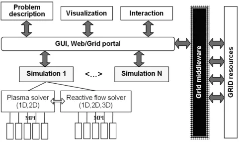
The application components perform one (or a few) of the following functions: problem description, simulation, visualization and interaction. This is schematically shown in Fig. 1, where we emphasize the simulation components.

Fig. 1. Functional scheme of the Virtual Reactor application

The core components are modules simulating plasma discharge, gas flow, chemical reactions and film deposition processes occurring in a PECVD reactor. The details on numerical methods and parallel algorithms employed in the solvers are described in [10]. The most important features relevant to the Grid implementation are as follows: for stability reasons, implicit finite volume schemes were applied, thus forcing us to use a sweep-type algorithm for solving equations in every “beam” of computational cells in each spatial direction of the Cartesian mesh. A special parallel algorithm was developed with beams distributed among the processors. Communications are organized exploiting a Master-Slave model, where at each simulated time step the Master prepares instructions for the Slaves, sends them the data to be processed, receives the results, and processes them before proceeding to the next step. The algorithm was implemented in an SPMD model, using the MPI message passing interface with MPI Barrier points for synchronization. Data exchange between the Master and the Slaves is repeated every time step, and simulation proceeds for thousands to millions of steps. In the testbed we use generic MPICH-P4 built binaries that can be executed on all the testbed machines using the Globus job submission service. To study the influence of various parameters on the simulated processes we run a number of simulations in parallel (shown in Fig. 1 as “Simulation 1” … “Simulation N” blocks) with the assistance of Nimrod-G [7].

To provide efficient execution of a parallel application on heterogeneous resources, it is needed to clearly understand the application performance dependencies on homogeneous resources first. This gives an insight into the application scalability, induced fractional overhead, dependencies of the amount of the communications and calculations on the number of processors used, etc. The results of such tests can help estimating and predicting the behaviour of the application on heterogeneous resources, thus simplifying the adaptation process.

3.2

Russian-Dutch Grid testbed infrastructure

Generally the infrastructure of a site within a Grid testbed can be of one of the following types depending on the underlying resources:

I. traditional homogeneous computer cluster architecture: homogeneous worker nodes and uniform interconnection links;

II. homogeneous worker nodes with heterogeneous interconnections; III. heterogeneous worker nodes with uniform interconnections; IV. heterogeneous nodes with heterogeneous interconnections.

A complete Grid infrastructure is always of the Type IV, characterized by severe heterogeneity with a wide range of processor and network communication parameters. As we show later in this paper, the type of resources allocated to a

parallel application significantly influences its performance, and different load balancing techniques shall be applied to different combinations of the resources.

Currently the Russian-Dutch Grid testbed consists of six sites with different infrastructures: Amsterdam-1 (contains 3 nodes, 4 processors) – Type IV; Amsterdam-2 (32 nodes, 64 processors) – Type I; St. Petersburg (4 nodes, 6 processors) – Type IV; Novosibirsk (4 processors) – Type II; Moscow-1 (13 nodes, 26 processors) – Type I; Moscow-2 (12 nodes, 24 processors) – Type I.

The Russian-Dutch Grid testbed is built with the CrossGrid middleware [5] based on the LCG-2 distributions and sustains the interoperability with the CrossGrid testbed. More detailed information on the RDG testbed can be found in [6]. The RDG Virtual Organization (VO) is included into the CrossGrid VO, thus allowing the RDG certificate holders to access some of the CrossGrid resources and services. The CrossGrid testbed consists of 16 sites with the infrastructures of all 4 types.

4

Application performance analysis on homogeneous sites

4.1

Benchmark approach

Benchmarking of a complex application is required to evaluate its performance and reveal the dependencies of its behaviour on the underlying infrastructure. We use a structural approach to benchmarking the Virtual Reactor as an example of a complex application. Within this approach, the overall functionality of the whole system is studied, followed by performance measurements of the individual components while they are not influenced by activities of the other components.

Benchmarking the components of a complex problem solving environment allows evaluating their performance depending on various parameters like types of input data and the resources used. This helps to predict the performance of a given component and use it for efficient resource allocation, thus improving the overall resource management within the whole application.

The earlier tests of the Virtual Reactor performed on the CrossGrid testbed showed that most of the interactive components of the Virtual Reactor do not put restrictions on the computer systems and network bandwidth and can be efficiently executed on distributed Grid resources [2]. Next, we focused on benchmarking of the simulation modules. Each simulation consists of two basic components: one for plasma simulation and another for reactive flow simulation (see Fig. 1). These two components exchange only a small amount of data every hundred or thousand time steps, therefore the network bandwidth is not critical for their communication. Finally, we concentrate on benchmarking the individual parallel solvers, starting from a 2D PECVD solver which maintains all the features of the 3D one but takes less time to estimate the solver behaviour on the Grid.

4.2

Benchmark setup

The goal of the benchmarking we carry out is to determine the scalability of the application, find out the limitations on the efficiency posed by the application architecture, resources and types of the simulations. Uncovering such details will allow us to optimize resource management strategy for allocating the application components within the whole Virtual Reactor problem solving environment.

The solver operates a reactor geometry that is composed of a number of connected blocks. Different types of simulation can be performed within a single geometry: a chemically inactive flow and a flow with chemical and plasma processes. Physically the problem type is determined by the gas mixture composition, temperatures, pressures, and the plasma discharge operation mode. From the computational point of view these types of simulations differ by the ratio of computations to communications: in case of simulating chemical processes the computational load is significantly higher.

We started from a light-weighted problem not simulating the chemical and plasma processes, with a simplified reactor geometry consisting of a single block that allows easy tracking of parameter influence on the execution time. To measure the dependency of the solver performance upon the input data, multiparameter variation has been applied. We measured the solver execution time, speedup and communication time depending on the combinations of input parameters: the computational mesh size, number of simulation time steps and number of processors.

The benchmark tests had to be automated because the parameter variation leads to a large number of job submissions. To solve this problem we have built an execution environment to support series of parameter-sweep Globus job submissions. The environment is generic and can be used for any kind of performance benchmarks with user-defined metrics and parameters to be analyzed. Within this environment, the application to benchmark is described using some templates that are filled with particular application data (e.g. Globus RSL template for job submission which also contains the list of input and output files). One of the functionalities of this execution environment is the support for parameter-sweep runs, analogous to what Nimrod-G or Condor-G provides. The advantage of our implementation is that we can specify the parameters (and their ranges) that shall be changed, as well as the characteristics to be measured and visualized automatically to analyze the influence of those parameters.

In these tests, a single-block topology was used. The block was subdivided into a (ncell x ncell) number of computational mesh cells, with ncell running from 40 to 100, thus forming 1600–10000 cells. We performed also some tests with real reactor geometries in order to check whether the reactor topology influences the parallel performance, since potentially it can introduce some load imbalance.

4.3

Influence of the number of time steps and reactor topology

Experiments with a different number of time steps showed that the execution time and other measured parameters are linearly proportional to the number of time steps, provided that this number is high enough and the standard output and hard disk operations are kept minimal (that means no excessive logging, nor any storing of the 2D fields or other additional files every time step). All the results presented below are measured for 100 time steps.

Along with the single-block geometry, we studied the performance of the solver with a complex multi-block PECVD reactor topology, which consists of an equivalent number of computational mesh cells. The results showed that all the measured characteristics of the solver behaviour (execution time, speedup, computation and communication time) on the same resources do not differ for the single-block and multi-block topologies of equal number of cells within 1% accuracy. This assures us that the parallel algorithm used in the solver provides a good load balancing even in cases of complex topologies. Further we test the influence of the problem size (the number of mesh cells) with the single-block reactor geometry, since it is easier to vary the mesh size arbitrarily with a single-block geometry than with a multi-block complex topology.

4.4

Speedup of the chemistry-disabled and chemistry-enabled simulations

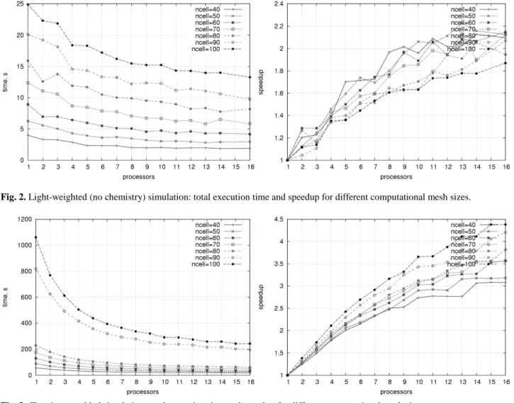
The measurements were carried out on all the Grid sites within the RDG testbed. The parallel solver showed a noticeable speedup on the Moscow and Amsterdam sites of Type I (homogeneous cluster with uniform communication links). Figures 2 and 3 demonstrate the total execution time and speedup of the parallel solver for different types of simulation: A chemistry-disabled “light-weighted” simulation (Fig. 2) and a chemistry-enabled “heavy” simulation (Fig. 3).

Fig. 2. Light-weighted (no chemistry) simulation: total execution time and speedup for different computational mesh sizes.

Fig. 3. Chemistry-enabled simulation: total execution time and speedup for different computational mesh sizes.

We observe different trends of the solver performance: for the light-weighted simulation, the speedup decreases with the increase of the mesh size (see the different curves in Fig. 2, right), while for the chemistry-enabled simulation, the speedup increases with the problem size increase (Fig. 3). The different absolute values of the speedup in Fig. 2 and 3 are mostly dependent on the resources: The results presented in Fig. 2 were obtained on the Moscow-1 site with slow interprocessor links, and Fig. 3 shows the results of the Amsterdam-2 site with fast communications. Different trends in the speedup dependency on the problem size are discussed and explained in detail in Sections 4.6 and 4.7.

The same parallel solver tested on homogeneous Grid sites with a higher ratio of the inter-process communication bandwidth to the processor performance achieved much higher speedups, for instance on lisa.sara.nl with Infiniband interconnections it was 3 times higher for the large problem size simulations. The type of MPI library also influences the parallel efficiency of a program: a specialized library optimized for the native communication technology (e.g. MPICH-GM for Myrinet communications on das2.nikhef.nl) increases the speedup up to two times compared to the generic MPICH-P4 or MPICH-G2.

4.5

Communication time trends

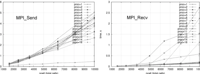
The time spent on inter-process communications within the solver is shown in Fig. 4 for different mesh sizes. The communication time was calculated as a sum of MPI Send/MPI Receive time on the master node over the total number of iterations.

Fig. 4. Dependency of the communication time on the computational mesh size for different number of processors (light-weighted simulation)

We observe that communication time grows super-linearly with the increase in mesh size, although the amount of data transferred is linearly proportional to the number of mesh cells. The exact understanding of this behaviour is not relevant and falls outside the scope of this paper. The fact that the time spent for sending the data is not equal to the time of receiving the data in Fig. 4 can be explained by the type of measurements: both plots represent the data sent or received by the master node only, as a synchronizing process. As one can see, the size of the received data (which represent the results of the calculations performed on the slave nodes) is significantly less than the data sent.

Some peculiarities in the communication time can be seen in Fig. 4, which are even more explicit in Fig. 5: (1) The communication time grows non-monotonically with the number of processors, but drops down a little on every processor with an even number; and (2) The time of MPI Receive calls is an order of magnitude higher for the larger meshes on the first few processors. These observations are discussed in Section 4.7.

Fig. 5. Dependency of the communication time on the number of processors for different computational mesh sizes (light-weighted

simulation)

4.6

Computation to communication ratio

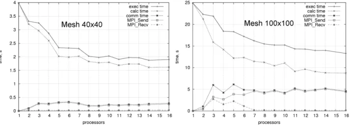
In Figure 6 the total execution time is presented along with the contributions of calculation and communication. For a smaller computational mesh (Fig. 6 left), the communication time makes a relatively small contribution to the total execution time even for a large number of processors involved. For a larger mesh (Fig. 6 right), communication makes up to 30% of the execution time. This result confirms that the network bandwidth is not sufficient for this type of problem (see also the explanations to Fig. 3).

Fig. 6. Total execution time and contributions of the calculation and communication depending on the number of processors for

different computational mesh sizes (light-weighted simulation)

As it was mentioned in the previous Section, the solver can simulate the chemical and plasma processes within the reactor along with the gas flow. Figure 7 demonstrates the ratio of computation to communication time for different mesh sizes with different types of the simulation. The higher the ratio is, the less communications are required, which obviously offers a better parallel efficiency and application scalability The ratios in Fig. 7 explain the different speedup trends observed in Fig. 2 and 3 for chemistry-enabled and chemistry-disabled (light-weighted) simulations. From the presented graphs we can see that the behaviour of this ratio does not depend on the mesh size for the chemistry-enabled simulations, while this behaviour for the light-weighted simulations significantly differs for small and large mesh sizes. For a small mesh size, the ratio stays decently high, and for 6 processors and more it reaches the level of the chemistry-enabled simulations. For a larger mesh, the computation/communication ratio for the no-chemistry simulations is very low, thus diminishing the overall parallel efficiency.

Fig. 7. The ratio of the computation to communication time for chemistry-enabled and light-weighted simulations

4.7

Discussion of the results for homogeneous resources

The results presented in Section 4.4 show that the parallel speedup is lower for a larger problem size (with more computational mesh cells) for the simulations of problems without chemical processes (see Fig. 2). This fact indicates that the ratio of the inter-process communication bandwidth to the processor performance was not high enough for light-weighted problems with relatively small number of operations per computational cell. It means that for optimal usage of the computing power, a large number of processors for one parallel run shall only be used for relatively small computational meshes. Thus the communication technology puts a limit to the scalability of the solver for this problem type. On the other hand, the simulation of the flow with chemical processes shows higher speedup with larger meshes

(see Fig. 3). Here the amount of computations brought by simulating the chemistry changes the behaviour of the solver qualitatively. This leads us to the conclusion that different resource allocation strategies should be applied for different types of simulation and meshes used.

The results in Fig. 5 reflect the network and nodes features of the tested Grid site:

1. Since the site consists of dual nodes, the network channels work more efficiently for data transfers between the Master and a Slave processor if a connection was already established with another Slave processor on the same node. This can be explained by implementation of the MPI library which saves network resources while opening and maintaining connections for concurrent processes on the same node.

2. The “peaks” of the MPI Receive time for the first few processors (see Fig. 5 right) are caused by the constraints on the portions of data that could be accommodated at once. The constraining factors could be the network bandwidth distribution, the processor cache size, the memory available on the node, or a combination of these factors.

5

Application performance on heterogeneous resources

5.1

Performance of the parallel solver on heterogeneous resources

The RDG Grid sites with heterogeneous processors and/or network links (Types II, III, IV) provided only a limited parallel speedup or even a slow-down of the original solver with a homogeneous parallel algorithm (data not shown). This was inevitable since, in addition to the low-bandwidth links, these sites are characterized by very diverse resources: the processor and network parameters differ by orders of magnitude for different nodes.

The solver parallel algorithm was originally developed for homogeneous computer clusters with equal processor power, memory and inter-processor communication bandwidth. In case of submitting equal portions of a parallel job to the nodes with different performance, all the fast processors have to wait at the barrier synchronization point till the slowest ones catch up, thus the effect of slow-down on heterogeneous resources is not surprising. The same problem occurs if the network connection from the Master processor to some of the Slave processors is much slower than to the others. As we have shown in the previous section, for communication-bound simulations (chemistry-disabled simulation with large computational meshes), the communication time on low-bandwidth networks is of the order of the calculation time, therefore the heterogeneity of the inter-processor communication links is a hindrance as considerable as the diversity of the processor power. One of the natural ways to adapt the solver to the heterogeneous Grid resources is to distribute the portions of job among the processors according to the processor performance and network connections, taking into account the application characteristics. To adapt the parallel solver, we applied the approach presented in Section 2.

5.2

Experimental results of the workload balancing algorithm

To illustrate the approach described in Section 2 we present the results obtained for different types of simulation (chemistry-disabled and enabled) of a reactor geometry with 10678 cells on the St. Petersburg Grid site. This site is heterogeneous in both the CPU power and the network connections of the processors (Type IV). There are two 1.8 GHz nodes (nwo1.csa.ru, nwo2.csa.ru) and two dual 450 MHz nodes (crow2.csa.ru, crow3.csa.ru), all having 512 MB RAM. One of the dual nodes (crow3.csa.ru) is placed in a separate network segment with 10 times lower bandwidth (10 Mbit/s against 100 Mbit/s in the main segment). The load balancing tests were performed with a moderate-size problem which does not pose restrictions on required memory, thus the memory influence parameter

c

_m was reduced to zero and the exploration was done for the application parameter

f

_c. The link bandwidth between the Master and Slave processors was estimated by measuring the time of MPI_Send transfers of a predefined data block (with the MPI buffer size equal to 106 of MPI_DOUBLEs) during the solver execution, after the resources have been allocated. In these measurements

the same logical network topology was used as employed in the solver. The CPU power and available memory were obtained by a function from the perfsuite library [11]. To validate the approach presented in Section 2 we applied the workload balancing technique for a single simulation running on different sets of heterogeneous resources. The estimation of performance for different possible values of the parameter

f

_c(hence different weighting and workload distribution) was carried out. For one simulation type we expect to obtain approximately the same value of the parameter

f

_c* (that provides the best performance, see Section 2) on different sets of resources. Figure 8 (left) illustrates the load-balancing speedup

Θ

achieved by applying the workload balancing technique for different values of the parameter

f

_c on several fixed sets of heterogeneous resources for a light-weighted (chemistry-disabled) simulation. In Table 1 we summarize the combinations of processors dynamically allocated in 4 tests (different sets of resources) and the weights assigned to each processor for the values of

f

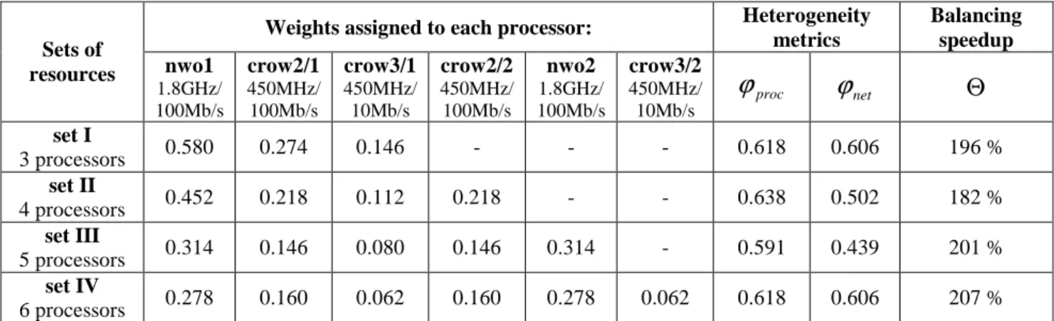
_c* providing the best execution time, thus the maximal balancing speedup (see Fig 8 left).

Weights assigned to each processor: Heterogeneity metrics Balancing speedup Sets of resources nwo1 1.8GHz/ 100Mb/s crow2/1 450MHz/ 100Mb/s crow3/1 450MHz/ 10Mb/s crow2/2 450MHz/ 100Mb/s nwo2 1.8GHz/ 100Mb/s crow3/2 450MHz/ 10Mb/s proc

ϕ

ϕ

net

Θ

set I 3 processors 0.580 0.274 0.146 - - - 0.618 0.606 196 % set II 4 processors 0.452 0.218 0.112 0.218 - - 0.638 0.502 182 % set III 5 processors 0.314 0.146 0.080 0.146 0.314 - 0.591 0.439 201 % set IV 6 processors 0.278 0.160 0.062 0.160 0.278 0.062 0.618 0.606 207 %

Table 1. Distribution of processors and balancing weights providing the best load balancing speedup for different sets of resources.

Figure 8 (left) shows that for a given simulation the best performance is delivered by weighting the resources with the value of

f

_c

≈

0.3-0.4. Noticeably, this corresponds to the value obtained for this simulation during the preliminary analysis on homogeneous resources (compare to results for similar simulations in Section 4.6, Fig. 7). The results show that the algorithm gives the increase of the balancing speedup

Θ

_{up to 207 percent compared to the initial} non-balanced version of the code (with homogeneous workload distribution) on the tested resource sets. We can see that the distribution of the workload proportional only to the processor performance (

f

_c

=

0

) also gives a significant increase of the performance, but introduction of the dependency on application specific communication/computation ratio

f

_c and resource infrastructure parameters

µ

_i adds another 40 percent to the balancing speedup

Θ

.

Fig. 8. Dependency of the balancing speedup

Θ

on the resource parameter

f

_c. Left: single simulation on different sets of resources..Right: different types of simulation on the same set of resources.

Figure 8 (right) shows the dependency of the balancing speedup

Θ

for different types of simulation (chemistry enabled or disabled) on the same set of resources (set III from Table 1). The chemistry-disabled simulation has a higher communication/computation ratio (as was shown also in Section 4.6, Fig. 7). This is clearly seen in the experimental results where chemistry-disabled simulation obtains the highest balancing speedup

Θ

_{at higher}

f

_cvalues. Moreover, the gain in the balancing speedup (maximal value of

Θ

) is higher for the simulation with a larger fraction of communications. These results illustrate that the introduced algorithm for resource adaptive workload balancing can bring a valuable increase in the performance for communication-intensive parallel programs running on heterogeneous resources.

5.3

Discussion and suggestions for generalized automated load balancing

The introduction of the load balancing technique allowed us to increase the efficiency of the parallel solver on heterogeneous resources. The proposed method of successive estimation of resource infrastructure parameters

µ

_i and further determination of the application specific

f

_c shows the possibility of automatic load balancing for applications which internal structure (computations and communications) is not known.

Analysis of the results achieved with the workload balancing algorithm suggested that the following issues shall be addressed in order to optimize the balancing technique:

1. To measure the inter-process communication rate, we sent a fixed amount of data from the Master to each Slave processor. However in some cases the response of the communication channels to the increasing amount of data is not linearly proportional as shown in Fig. 4. For the slower networks this tendency is even more pronounced. This brings us to a conclusion that the amount of data sent to measure the links performance shall be close to the amount really transferred within the solver for every particular mesh size, geometry and solver type. Another option to estimate the inter-processor communication rate is to analyze the iteration data transfer time during the actual execution. However, this requires significant code modifications and might be undesirable.

2. To properly take into account the memory requirements of each particular instance of a parallel solver, similar reasoning shall be applied as for selecting

c

_p and

c

_n: the choice of the

c

_m coefficient, setting the significance (priority) of the memory factor influence on the application performance, must depend on the type of resources assigned, analogous to the

c

_p.

3. The specialty of the memory factor is that in addition to this resource-dependency it is strongly influenced by the application features. To take into account the memory requirements of a parallel solver, the weighting algorithm must be enriched by the function measuring the memory requirements per processor for each simulation on each set of resources. In case of sufficient memory on allocated processors, the load balancing can be performed taking into account all the factors (CPU, memory and network) where memory factor is a constraint. After this, another check of meeting the memory requirements on each processor must be performed. In the unfavourable case of insufficient memory on some of the processors, they must be disregarded from the parallel computation or replaced by other, better suited processors. This must be done preferably outside the application, on the level of parallel job scheduling and resource allocation. This brings us to the conclusion that ideally a combined technique shall be developed, where the application-centred load balancing approach is coupled with a system-level resource management.

6

Conclusions

In this paper we address the issue of porting distributed problem solving environments to the Grid, using Virtual Reactor as an example of a complex application. One of the most challenging problems we encountered was porting parallel modules from homogeneous cluster environments to heterogeneous resources of the Grid, specifically the issue of keeping up a high parallel efficiency of the computational components. This problem arises for a wide class of parallel programs that employ homogeneous load distribution algorithms. To adapt these applications to heterogeneous Grid resources, we developed a theoretical approach and a generic workload balancing technique that takes into account specific parameters of the Grid resources dynamically assigned to a parallel job, as well as the application requirements. We validated the proposed algorithm by applying this technique to the Virtual Reactor parallel solvers running on the Russian-Dutch Grid testbed. It is worth noting that the load balancing speedup goes through a maximum at fc = fc* as

shown in Fig. 8. This indicates that the load balancing strategy does find an optimum in the complex parameter space of the heterogeneous application/architecture combination. The clear maximum gives an unbiased guide towards automatic load balancing. The developed approach is well suited for either static or dynamic load balancing, and can be combined with the Grid-level performance prediction models or application-level scheduling systems [18,19]. To further explore this new load balancing approach, we are currently working on the comparison of the theoretically derived optimization parameters for some specific topologies of parallel applications with those predicted by our heuristic algorithm.

In order to optimize the resource management strategy of mapping the distributed components of the application problem solving environment, we benchmarked the individual components of the Virtual Reactor on a set of diverse Russian-Dutch Grid resources, and extensively studied the behaviour of the parallel solvers with various problem types and input data on different resource infrastructures. The results clearly show that even within one solver different trends can exist in the application requirements and parallel efficiency depending on the problem type and computational parameters, therefore distinct resource management and optimization strategies shall be applied, and automated procedures for load balancing are needed to successfully solve complex simulation problems on the Grid. Acknowledgments. The authors would like to thank Irina Shoshmina, Alfredo Tirado-Ramos and the RDG Grid deployment team for their assistance. The research was conducted with financial support from the Dutch National Science Foundation NWO and the Russian Foundation for Basic Research under grants number 047.016.007 and 047.016.018, and with partial support from the Virtual Laboratory for e-Science Bsik project [8].

References

1. www.cfdrc.com, www.fluent.com, www.semitech.us, www.softimpact.ru

2. V.V. Krzhizhanovskaya, P.M.A. Sloot, and Yu. E. Gorbachev. Grid-based Simulation of Industrial Thin-Film Production. Simulation: Transactions of the Society for Modeling and Simulation International, V. 81, No. 1, pp. 77-85 (2005)

3. V.V. Krzhizhanovskaya, M.A. Zatevakhin, A.A. Ignatiev, Y.E. Gorbachev, W.J. Goedheer and P.M.A. Sloot. A 3D Virtual Reactor for Simulation of Silicon-Based Film Production. Proceedings of the ASME/JSME PVP Conference. ASME PVP-Vol. 491-2, pp. 59-68, PVP2004-3120 (2004)

4. proj-openlab-datagrid-public.web.cern.ch, www.nbirn.net, www.fusiongrid.org, www.globus.org/alliance/projects.php, cmcs.ca.sandia.gov, www.us-vo.org

5. The CrossGrid EU Science project: http://www.eu-CrossGrid.org 6. High Performance Simulation on the Grid project: http://grid.csa.ru 7. Nimrod-G: http://www.csse.monash.edu.au/~davida/nimrod/ 8. The Virtual Laboratory for e-Science project: http://www.vl-e.nl

9. David W. Walker, Maozhen Li, Omer Rana, Matthew S. Shields, and Y. Huang. The software architecture of a distributed problem-solving environment. Concurrency - Practice and Experience, 12(15):1455-1480, 2000.

10. V.V. Krzhizhanovskaya et al. Distributed Simulation of Silicon-Based Film Growth. Proceedings of the 4th _{PPAM conference,}

11. R. Kufrin. PerfSuite: An Accessible, Open Source Performance Analysis Environment for Linux. 6th International Conference on Linux Clusters. Chapel Hill, NC. (2005)

12. J.D. Teresco et al. Resource-Aware Scientific Computation on a Heterogeneous Cluster. Computing in Science & Engineering, V. 7, N 2, pp. 40-50, 2005

13. R. David et al. Source Code Transformations Strategies to Load-Balance Grid Applications. LNCS vol. 2536, pp. 82-87, Springer-Verlag, 2002

14. A. Barak,, G. Shai,, and R. Wheeler The MOSIX Distributed Operating System, Load Balancing for UNIX, LNCS, vol. 672, Springer-Verlag, 1993

15. K.A. Iskra; F. van der Linden; Z.W. Hendrikse; B.J. Overeinder; G.D. van Albada and P.M.A. Sloot: The implementation of Dynamite - an environment for migrating PVM tasks, Operating Systems Review, vol. 34, nr 3 pp. 40-55. Association for Computing Machinery, Special Interest Group on Operating Systems, July 2000.

16. G. Shao, R. Wolski and F. Berman. Master/Slave Computing on the Grid. Proceedings of Heterogeneous Computing Workshop, pp 3-16, IEEE Computer Society (2000)

17. S.Sinha, M.Parashar. Adaptive Runtime Partitioning of AMR Applications on Heterogeneous Clusters. In Proceedings of 3rd IEEE Intl. Conference on Cluster Computing, pp435-442, 2001

18. F. Berman, R. Wolski, H. Casanova, W. Cirne H. Dail, M. Faerman, S. Figueira, J. Hayes, G. Obertelli, J. Schopf, G. Shao, S. Smallen, N. Spring, A. Su, D. Zagorodnov. Adaptive Computing on the Grid Using AppLeS. IEEE Trans. on Parallel and Distributed Systems, vol. 14, no. 4(2003) 369—382

19. X.-H. Sun, M. Wu. Grid Harvest Service A System for Long-Term, Application-Level Task Scheduling. Proc. of 2003 IEEE International Parallel and Distributed Processing Symposium (IPDPS 2003)(2003)

20. G. Fox, M. Johnson, G. Lyzenga, S. Otto, J. Salmon, and D.Walker. Solving Problems on Concurrent Processors, volume 1, Prentice-Hall, 1988.

21. J.F. de Ronde; A. Schoneveld and P.M.A. Sloot: Load Balancing by Redundant Decomposition and Mapping, Future Generation Computer Systems, vol. 12, nr 5 pp. 391-407, April 1997

22. J.F. de Ronde. Mapping in High performance Computing. A case study on Finite Element Simulation, PhD thesis, University of Amsterdam, 1998

23. Chin Lu, Sau-Ming Lau. An Adaptive Load Balancing Algorithm forHeterogeneous Distributed Systems with Multiple Task Classes, International Conference on Distributed Computing Systems (ICDCS'96)

24. Zhiling Lan, Valerie E. Taylor, Greg Bryan. Dynamic Load Balancing of SAMR Applications on Distributed Systems, Proceedings of the 2001 ACM/IEEE conference on Supercomputing

25. Yongbing Zhang, K. Hakozaki, H. Kameda, K. Shimizu. A performance comparison of adaptive and static load balancing in heterogeneous distributed systems, the 28th Annual Simulation Symposium, p. 332, 1995.