CREW OPTIMIZATION IN PLANNING AND CONTROL OF EARTHMOVING OPERATIONS USING SPATIAL TECHNOLOGIES

(1)

ITcon Vol. 12 (2007), Moselhi and Alshibani, pg. 121

CREW OPTIMIZATION IN PLANNING AND CONTROL OF

EARTHMOVING OPERATIONS USING SPATIAL TECHNOLOGIES

SUBMITTED: July 2006 REVISED: January 2006

PUBLSIHED: February 2007 at http://itcon.org/2007/7/ EDITOR: B-C Björk

Osama Moselhi, Professor Dr.

Department of Building, Civil & Environmental Engineering, Concordia University, Montreal, Canada email: [email protected]

Adel Alshibani, PhD Candidate

Department of Building, Civil & Environmental Engineering, Concordia University, Montreal, Canada email: [email protected]

SUMMARY:This paper presents a model designed for planning, tracking and control of earthmoving

operations. The paper briefly describes the main modules and components of the developed model to maintain continuity and focuses primarily on the Crew Optimization Module of the model. The proposed model utilizes and combines genetic algorithm and spatial technologies including Global Positioning System (GPS) and Geographic Information System (GIS) to support the management functions of the developed model. The model assists in selecting near optimum crew formations in the planning phase using genetic algorithm (GA) supported by GIS. GA is used in conjunction with a set of rules developed to speedup the optimization process and to avoid generating and evaluating hypothetical and unrealistic crew formations. GIS is employed to automate data acquisition and to analyze the collected spatial data. GPS is used for site data collection and for tracking construction equipment in near real time. The model accounts for resources that are available to contractors and it is capable of reconfiguring crew formations dynamically during the construction phase while site operations are in progress. The optimization of crew formation considers: 1) construction time, 2) construction cost, or 3) construction time and cost. The model is also capable of generating crew formations to meet, if possible, specified time and/or cost constraints. It is capable of generating graphical and tabular reports with various degrees of detail to suit the requirements of project teams. At the core of the proposed model is its central database that houses the needed data for the analysis. The developed model has been implemented in prototype software, using object-oriented programming and Microsoft Foundation Classes (MFC), and has been coded using visual C++ V.6.The developed software operates in Microsoft Windows’ environment. To illustrate its capabilities in crew optimization, an example project, drawn from the literature, is analyzed.

KEYWORDS: planning, tracking, earthmoving, spatial technologies, genetic algorithm.

1. INTRODUCTION

In construction projects that involve earthmoving operations, project managers are under pressure to improve productivity, efficiency, and safety. Achieving these goals requires an effective planning, tracking and control system. The main goals of planning earthmoving operations are to: (1) optimize the use of available resources; (2) balance resources throughout the project duration and/or its development stage; (3) select suitable equipment for the work at hand, taking into consideration construction site conditions and the mechanical specifications of equipment to maximize productivity and consequently maximize profit of contractors; and (4) complete projects with least cost and within the given targeted project duration (Reda, 1990). Considerable work has been carried out to develop models for managing earthmoving operations so as to achieve the previous stated goals. Some of these models use queuing theory (Halpin and Woodhead, 1976) and others use simulation (Oloufa, 1993; AbouRizk and Hajjar, 1998; Marzouk and Moselhi, 2002). These systems lack the ability to: (1) consider the interaction among the individual pieces of equipment in a fleet, as in the case of Fleet Production and Cost Analysis (FPC) software (Caterpillar Inc. 1998); (2) evaluate, concurrently, different fleet scenarios and provide reliable estimates of haulers travel time, as in the case of MicroCYCLONE (Halpin and Riggs, 1992); and (3) dynamically reconfiguring crew formation while site operations are in progress.

(2)

Further to the above, tracking and controlling these operations require close monitoring of the equipment involved. The close monitoring process needs timely collection of a huge amount of data to estimate the crew actual productivity. Estimating actual productivity is a key element in estimating the time and cost required to complete construction operations (Oglesby et al 1989).Traditionally, site data collection and analysis used in this class of projects have been carried out manually and have been limited to the involvement of human observers. Using manual methods has been recognized to be time consuming, resulting in tardy corrective actions with undesirable cost consequence (Sacks et al, 2002). For this reason, an effective control system should use automated site data collection tools that are able to gather large volumes of necessary data in a timely manner. Spatial technologies have been used, in recent years, in many aspects of earthmoving operations such as: collision avoidance of earthmoving equipment (Lothon et al, 1996 and Oloufa et al, 2002), calculating durations of earthmoving activities (John et al, 2005), automating data acquisition and analysis for planning and scheduling of highway construction operations (Hassanien et al, 2002). None of the previously referred to work focuses on tracking and control of earthmoving operations based on data collected by GPS. This paper presents a model designed for planning, tracking and control of earthmoving operations using spatial technologies. The paper describes briefly the model and its main modules and focuses on its Crew Optimization Module.

2. SYSTEM OVERVIEW

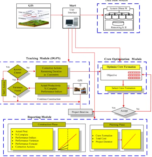
A flexible system utilizing spatial technologies to plan, track, and control earthmoving operations is presented. Unlike current systems, the proposed system optimizes the use of available resources at the planning phase and during construction while the project is progressing, automates site data collection and processing, and tracks and monitors the construction equipment involved in near real time. The system consists of four main modules and one algorithm. They are: (1) database module, (2) crew optimization module, (3) tracking and control module, and (4) reporting module. The algorithm is named “Path Finder”. Fig. 1 depicts the systems main modules. It should be noted that, the red lines represent the logic flow of computation processes within the system.

(3)

The system retrieves the necessary data from three sources in addition to the data entered by the user. The first source is the system database. The second source is the GIS through the use of the developed Path Finder algorithm. The third source is the data collected by GPS receivers. In this paper the database and tracking and control modules are briefly described and the crew optimization module is described in details.

2.1 Database module

The database module is of a relational type designed using Microsoft Access Database Management System. A relational database management system is used in view of its combination of power, simplicity, and ease of use (Kim et al 1989). This design allows all modules and Path Finder algorithm to be integrated easily. The proposed database module is based on that developed by Hassanien (Hassanien 2002). The database module stores the data needed for planning, tracking and control. These data can be clustered into:

• Resources data: 1) own equipment; 2) own labour force; 3) subcontractors; and 4) equipment suppliers. The equipment data include available equipment and the respective date of availability of each equipment. It also contains some other relevant information such as: equipment model, capacity, hourly fuel consumption, ownership, and operating cost. These data were mostly obtained from the equipment manufacturer. Equipment types are chosen based on those that are most often employed in this class of projects.

• Project data: 1) installed quantities and planned and actual cost, 2) the data collected by GPS receivers (positioning, date, time, and velocity).

• Soil data properties of different types of soil such as shrinkage and swell factors.

2.2 Tracking and control module

In an effort to circumvent the previously stated limitations of current control systems, the proposed system uses spatial technologies (GIS and GPS) to automate: 1) site data collection and acquisition; 2) estimate actual crew productivity; 3) measure project performance at the report date and forecast its status at completion, 4) detect causes behind unacceptable performance and to suggest corrective actions, if needed, and 5) generate a progress reports. The module retrieves the needed data from two sources. The first source is the data collected by GPS. This data contains positioning data for moving equipment such as altitude, longitude, latitude, date, speed, and time. The second source is the data stored in the central database. This data contains as-planned and actual data such as productivity, cost, and installed quantities. Having retrieved the needed data, the tracking module estimates actual productivity at the equipment level and at the crew level using the data collected by GPS receivers. The project performance indices are then calculated by comparing actual with as planned performance. If these indices fall within an unacceptable range, the module offers two options based on the causes of

unacceptable performance. If the cause(s) is (are) known, such as inclement weather and/or a strike, the user can take the appropriate corrective actions. Otherwise the module calls the optimization module to reconfigure the crews being used.

One of the interesting features of the proposed module is that it estimates actual productivity using data collected by GPS instead of data collected by human observers on site. The module estimates the crew actual productivity at a construction site by carrying out two steps: 1) it maps moving equipment by transforming its GPS

positioning data (Longitude, latitude, speed, time, and direction) into Geographic Information System (GIS) to develop a graphical presentation; 2) it analyzes these data to account for the number of cycles (trips) that certain equipment makes within a particular period of time. Having determined the cycle time and number of trips, actual productivity rates can then be estimated considering the characteristics of each construction equipment being tracked. Actual productivity can be estimated, in this case, as follows:

CF * Capacity Heaped ) Trips/Hr of (No Unit Hauling of No P/Hrs= × × (1) Where:

P/Hrs : The estimated actual productivity per hour

CF : Correction factor, it includes the efficiency factor, the fill factor, Job and management conditions, etc.

With minor modifications, Eq.1 can be applied to similar equipment such as compactors, graders, paving equipment, and rollers.

(4)

3. CREW OPTIMIZATION MODULE

Selection and optimum use of available resources are critical tasks for project management teams in heavy civil engineering projects. It has been reported, however, that no model can predict the output of such operations with a satisfactory degree of confidence in all situations (Marzouk et al 2000). In the present system, a Crew

Optimization Module is developed to optimize the use of available resources by optimizing crew formations and selecting the most suitable equipment for the work at hand. The module utilizes genetic algorithm as an

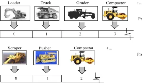
optimization tool supported by Path Finder algorithm developed in GIS environment. Genetic algorithm resemble the biological evolution principle of survival of the fittest (Holland 1992; Coley 1999). They follow random search techniques. The development of the optimization module as well as the genetic operators and fitness functions are descried below. Fig. 2 depicts the composition of the developed chromosomes of two predefined crews.

FIG 2: Developed chromosome

As presented in Fig. 3, the crew optimization module is composed of Genetic Algorithm, Path Finder Algorithm, and Database sub-Module. The Genetic Algorithm is used to search for feasible near optimum solutions. The Path Finder Algorithm is responsible for feeding the module with the data pertinent to travel roads, borrow pits and landfills. The Path Finder algorithm considers different borrow pits; landfill sites, travel paths and it selects the optimal path that suits the considered crew and offers the shortest travel and return time. The database provides this module with access to the data pertinent to available equipment and soil types. The module is capable of carrying out two kinds of optimization search. The first is “guided search”; in which the module searches only among equipment identified by the user. The second search is “an open search”; in which the module searches among all available resources in the resources’ database. In this case, the module is capable of reconfiguring crews with different equipment models.

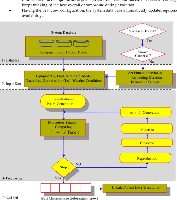
In addition to the optimization of crew formations in the planning phase, the module is capable of reconfiguring crews during construction dynamically while the project is progressing. This is carried out in an effort to support the generation of likely corrective action when there is deviation in the cost performance index (as planned cost/actual cost) and/or the schedule performance index (as planned working hours/actual working hours); depending on the optimization goal. In this case, the module considers the remaining time and/or cost to completion as constraints within which the project must be completed. It sets the fitness function to the value of the remaining time and/or cost to completion so that the algorithm reconfigure crews in order to meet these project constraints .Since precise constraints can not be always satisfied; the module can reconfigure crews to meet the constraints within time and/or cost ranges. Otherwise, it will alert the user to the need of considering crews beyond these stored in the database. Fig. 4 represents the crew optimization procedure during construction phase.

(5)

i=

i+

1

FIG. 3: Crew optimization module

The module takes the following steps to optimize crew formation:

• The module starts by accepting user entry data .This data include optimization goal, scope of work, daily and monthly working hours, indirect cost (daily mobilization, operation, and field expenses cost), soil types, and search type.

• Upon completion of step 1, the module first generates the initial population based on the user selection of predefined crew formations. In each formation, the module offers the user two kinds of crews. The first involves loading units, trucks, and support equipment. The second involves scrapers, pushers, and support equipment.

(6)

• The module then starts calculating the planned productivity for the loading and hauling unit by picking the number and the model of these units. The data required for this calculation are retrieved from two sources: 1) system database (equipment data including hourly cost, capacity, and speed, etc), 2) GIS (Path Finder Algorithm). The Path Finder Algorithm supports the

optimization module by selecting the optimal path from borrow pits to landfills. The optimal path offers the shortest travel and return time and consequently maximizes productivity.

• Having calculated the planned productivity for the hauling and loading units, the server waiting time is determined and added to the fitness function. The genetic algorithm then evaluates the fitness based on the optimization goal and save the best chromosome achieved. The algorithm keeps tracking of the best overall chromosome during evolution.

• Having the best crew configuration, the system data base automatically updates equipment availability. Stop ? Reproduction Mutation (n + 1) Generation Evaluation Fitness Computing ( Cost &Time)

Initialization ( N) th Generation

NO

Yes

Best Chromosome (reformation crew)

Update Project Data (Base Line) Equipment $, Prod, No Equip, Model

Quantities, Optimization Goal, Weather Conditions System Database

Remaining Duration Remaining Budget

No Yes

Set Fitness Function =

Equipment, Soil, Project DBase

1- Database 2- Input Data 3- Processing 4- Out Put Variances Found? Known Cause(s) ? Crossover

FIG. 4: Crew optimization procedure during construction phase

3.1 Path finder algorithm

The Path Finder Algorithm is developed mainly to enhance the crew optimization module. The algorithm analyzes the collected spatial data to find the optimal path for the equipment under consideration. It searches among many paths predefined earlier by the user. As presented in Fig. 3, the algorithm finds the optimal path by taking the following steps:

(7)

• It starts by accounting all available paths defined by the user at an early stage.

• The algorithm then retrieves the positioning data(X, Y, and Z) for each path individually. • Having the positioning data is retrieved; the algorithm then finds the relation between longitude

and latitude with altitude to find gradient resistance.

• The algorithm after that calculates the rolling resistance. The data required for calculating the rolling resistance (i.e. equipment weight and soil type) is retrieved from the system’s database. The rolling resistance can be expressed as follow:

RR=

(

40+(30×TP)

)

×GVW

(2) Where:

RR : Rolling resistance in pounds.

TP : Tire penetration in inches and it depends on soil type.

GVW : Gross vehicle weight in tons retrieved from system database.

• Having the total resistance (rolling resistance + gradient resistance) is determined; the algorithm then calculates the travel and return time and productivity of the considered hauling unit and saves these outputs.

• If the last path has not reached, repeat step 2 (loop).

• Having considered all paths, the algorithm then selects the path with the shortest travel and return time as the optimal path.

• The Path Finder Algorithm then feeds the genetic algorithm the data pertinent to the path identified in step 7 to continue its search for optimum crew formations.

3.2 Algorithm design

Genetic algorithm is used to provide near optimum solution in selecting of crew configuration. In an effort to speed up the GA operations and in order to circumvent the independency limitations in GA for solving this type of optimization problem, waiting time rule has been developed. This rule is described in details in following sections.

Populations and chromosomes are first generated and then tested for their respective fitness. The populations are generated via a set of genetic operators such as selection, crossover, and mutation (Holland, 1992). The selection process is carried out to choose a pair of chromosomes in order to perform the crossover process. In The

selection operations, chromosomes are randomly picked form within the top 25% of the population as it can be seen in Appendix A. After selecting a pair of chromosomes (parents), the crossover function randomly chooses whether the value for each gene in the offspring comes from parent1 or parent2. Each parent has an equal chance. After the creation of a new population, the mutation process is carried out in an effort to avoid local minima and to ensure that newly generated populations are not uniform and incapable of further evolution (Holland 1992). The mutation function adds a Gaussian distributed random value to the gene located at gene number. The new gene value is clipped if it does not fall between the user-specified boundaries. Additionally, the check for matching chromosome function has been used to check if a chromosome was present in the last population before evaluating it. If the last population contained an identical chromosome, the fitness is simply copied from the last population instead of computing it again. This function significantly speeds up the evolution.

3.3 Fitness function

The crew optimization module evaluates the fitness by calculating the productivity of each gene (equipment) in the selected crew (chromosome) based on a generated number for the equipment in that gene. The module picks out the gene with a minimum productivity to control the whole crew productivity.

In addition, the module uses the developed server waiting time rule in an effort to speedup the optimization process and avoid generating and evaluating hypothetical and unrealistic crew formations. It helps the genetic algorithm to select crew formations in which the number of servers matches well the number of customers and vice versa. The closer waiting time is to zero; the better is the match between the servers (loading units) and the customers (hauling units). The value of waiting time is used to evaluate the fitness and is not intended to be used to calculate the project time. It is calculated as follow:

(8)

X = (((Loader_Productivity*chromosome.genes(0).getValue())/

(TruckProductivity*chromosome.genes(1).getValue())) –

(3) (chromosome.genes(1).getValue()))*(loading_Time/60.0));

The module calculates the project total time based on the calculated daily production of the selected crews. Consequently, the time required to complete the work is calculated considering the total scope of work. On the other hand, the total cost is calculated by adding the direct cost if the objective is to minimize cost and by adding direct and indirect cost if the objective is to minimize project time and cost. The direct cost is estimated based on the time required by the selected crews to complete the project scope of work. The equipment direct cost includes owning and operating cost. The indirect cost has two components: one is time depended and the other is time independent. They include the use daily cost, if applicable, mobilization cost, field expenses cost, overhead and taxes cost. The fitness estimation is described based on the optimization goal as follows:

Minimize project time

In this case, the module search and select the crew that minimizes the project time regardless of it associated cost but the match between the loading and hauling unit is still accounted for.

X Min_Prod pe_Work Actual_Sco ) fittness ( Total_Time _⎟⎟+ ⎠ ⎞ ⎜⎜ ⎝ ⎛ = (4) Where:

Total_Time : Project total time is calculated by fitness function.

pe_Work

Actual_Sco : Quantity of earth to be moved.

Min_Prod : Productivity of equipment that controls the crew (chromosome);

X : Server waiting time. Minimize project cost

In this case, the module searches and selects the crew that minimizes the project cost regardless of it associated time. Cost Direct me Project_Ti Total_Cost= × (5) ⎟ ⎟ ⎠ ⎞ ⎜ ⎜ ⎝ ⎛ ∑ = ⎟⎟ ⎠ ⎞ ⎜⎜ ⎝ ⎛ × × = t 1 i _{Min_Prod} pe_Work Actual_Sco i NE i EHC (fittness) Total_Cost ₍₆₎ Where:

Total_Cost : Project total cost

EHC : Equipment hourly ownership and operating cost.

NE : Number of pieces of equipment associated with each type. Minimize project time and cost

Cost plus time is treated in manner similar to what is known as A+B bidding (Hassanien, 2002), which was introduced to minimize public inconvenience arising from construction operations in urban centres. This can be achieved by encouraging contractors to develop project plans that are capable of shorting project duration.The module here uses a multi objective function to minimize project cost and time. In this case, the optimization module takes into consideration the daily user cost as decision variable.

⎟ ⎠ ⎞ ⎜ ⎝ ⎛ _⎟ ⎠ ⎞ ⎜ ⎝ ⎛ _× + ∑ = × × = DH DUC me Project_Ti t 1 i EHCi NEi Project_Time Total_Cost (7) Where:

DH : Scheduled working hour per day.

EHC : Equipment hourly ownership and operating cost.

NE : Number of pieces of equipment associated with each type.

(9)

4. COMPUTER IMPLEMENTATION

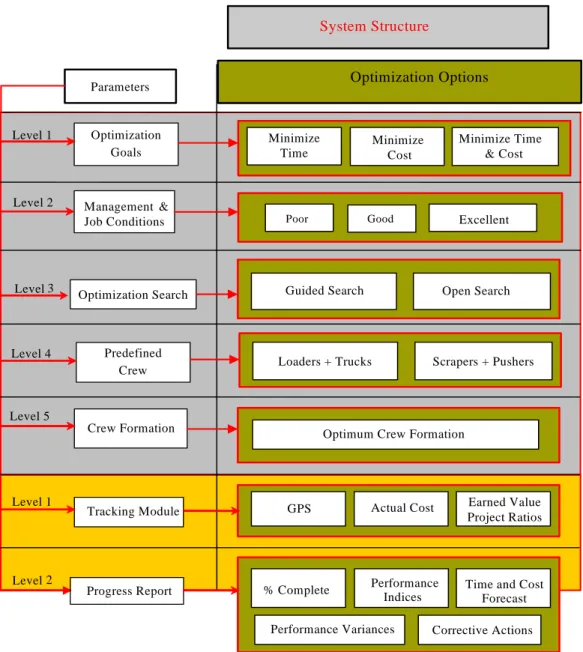
A prototype software package has been developed to automate planning, tracking, and controlling of earthmoving operations as proof of concept. The software composes of two components that can operate independently or interactively. The first component carries out the optimization of the crew formations at planning phase and during the construction. The second component tracks and controls the earthmoving operations during construction. The software has been developed using Microsoft Visual C++ by employing Microsoft Foundation Classes (MFC) and ESRI Mapobjects library. The system architecture is designed to allow flexible expansion and change without affecting the rest of the system. Adding a new module for another type of project planning and control such as highway construction, however, can be easily integrated within the system. Fig. 5 represents a part of the developed system’s breakdown structure, which incorporates seven levels. At the core of the system is its database. The database is designed in a relational database using Microsoft Access Database Management System. This design allows all modules and algorithm to be integrated easily. It stores the data needed for planning, tracking and control.

Optimization Search Level 3 Parameters Optimization Goals System Structure

Level 1 Level 2 Level 5 Level 2 Crew Formation Tracking Module Progress Report Minimize Time Minimize Cost Minimize Time & Cost Poor

Optimum Crew Formation

% Complete Performance

Indices

Time and Cost Forecast Corrective Actions Performance Variances Optimization Options Scrapers + Pushers Loaders + Trucks Predefined Crew Level 4 Level 1 Excellent

Guided Search Open Search

Actual Cost

GPS _{Project Ratios}Earned Value

Management &

Job Conditions Good

FIG. 5: System breakdown structure

Upon the completion of the input data and selection of some options, the optimization module triggers and automatically transfers the required data from the database to VC++. In VC++, the user is requested to key in additional data related to management and job conditions, project indirect costs, selections of hauling routes, etc.

(10)

The system then automatically progresses with the optimization analysis, generates the optimal crew formations, and estimates project time and cost.

The optimization process is carried out through a set of Dialog Windows that interact directly with the user. Having generated the optimal crew formations and after starting construction, the tracking software can then be activated through setting out tracking parameters. It automatically progresses with the crew productivity analysis, measures the project schedule and cost status at the report date, and forecasts it at completion. The analysis is essentially performed based on the user selection of tracking parameters and the level of detail required. The project status is represented by the cost performance index (CPI), the schedule performance index (SPI), the productivity performance index (PPI), and associated variances and forecasts. The system calculates these indices using the earned-value concept or project ratios techniques. Fig. 6 represents the data flow of the proposed system. It starts with the data entered by the user; data retrieved from the system database, and the data collected by GPS during construction phase.

Start

Select Optimum Crew Formation

Planning Phase Collect GPS Data

Tabular Graphical Reporting Module Database M GUI End Tracking Module Construction Phase - % Complete - Actual Cost - Estimate Actual Prod - Measure Perform Indices - Time & cost Variances - Time & cost Forecast - Corrective Actions Soil data - Shrinkage Factor - Swell Factor Equipment - Number - Capacity - Speed,…. Predefined Crews - Loaders +Trucks + Supporter - Scrapers +Pushers +Supporter

Project Data - As Planned &Actual $ - As Planned & Actual Quant - Time

User Input Data - Indirect Cost - Scope of Work - GAs Parameters

Crew Formation Module

Reasons Knowledge Base

FIG. 6: Data flow in proposed model

Fig. 7 depicts the input and the output of the proposed system. The input data can be entered at two phase. The first phase is planning phase to optimize crew formations. The second phase is construction to estimate actual performance and measure the project status. The output is represented by crew formations and project cost and time at planning phase, whereas the output of tracking module at construction phase is represented by

(11)

FIG. 7: Input and output data of the proposed system

4.1 Graphical user interface

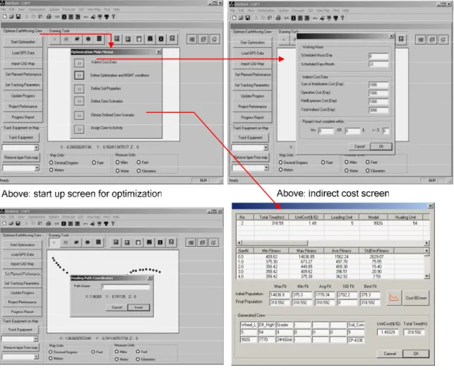
The Graphical User Interface contains a series of Dialog Windows for the user to select from. The user interface incorporates menus, toolbars, and dialog windows in addition to drawing tools. The implementation of the Graphical User Interface (GUI) is carried out in a way that facilitates data entry and minimizes redundant data input. Fig. 8 shows the system main dialog.

The dialog windows are built utilizing object–oriented programming and employing Microsoft Foundation Classes (MFC). This enables the utilization of predefined classes to carry out several functions.

FIG. 8: System main dialog

Output Data - Crew Formation - Project Time - Project Cost Input Data Tracking Module Performance Forecast -Optimization Module Input Data Equipment H. Cost No of available Resources Scope of Work

Soil (Swell &Shrinkage F)

Indirect Cost

Daily Working Hours Weekly Working Days

Surface Conditions

Management & Job Conditions

Travel Path - GPS Data - Actual Cost Performance Indices Performance Variances -Corrective Actions Equipment Model - Actual Quantities Construction Phase Planning Phase

(12)

The main screen of the system consists of one main view in the centre to display a project map. The central view is designed to occupy approximately 60% of the main screen displaying a mapping area where GPS data is displayed as layers. The left side of the screen displays the table of contents of the project layers (moving construction equipment at site). The right side displays the access to system different modules. Different class controls are used to facilitate the interaction between the user and the system’s modules. These controls include Pushbuttons, Combo boxes, Check boxes, Radio buttons, and Map control. Fig. 9 shows optimization prototype main Dialogs Windows and Output respectively.

FIG. 9: Optimization prototype main screens

5. APPLICATION EXAMPLE

To illustrate the ability of the proposed system in selecting near optimum crew configuration in earthmoving operations, an example project, drawn from the literature (Marzouk et al 2002), is analyzed. The project involves moving of 3210000 Cubic Meter of dry clay from borrow bit a quarry to dam site. The crew consists of loading units, hauling units, spreaders, and compactors. Table 1 and Table 2 represents haul road characteristic and characteristic of crew equipments respectively. Table 3 represents genetic algorithm parameter values used in the analysis. The system has been tested in selecting crew configuration to minimize project time, project cost, and project time and cost. As presented in Table 4 and Fig. 10 and Fig. 11, applying the waiting time rule guarantees that the number of trucks matches well the number of loaders and the number of graders matches well the number of trucks, and the number of compactors matches well the number of the graders. For example, In case of minimizing time, the system selects the crew that is capable of maximizing productivity and consequently minimizing project time regardless of the associated cost. The system selected the maximum number of the

(13)

available loader (8 loaders) and select just (37) trucks, 7 graders, and 6 compactor. The system selects just 37 trucks of the available 60 because of applying the server waiting time rule developed in this study. In other word selecting all available trucks will not improve crew overall productivity and consequently will not further minimize project time In case of minimizing project cost, the system selects crew that minimizes project cost regardless of the associated time. Here again the waiting time rule is applied to avoid selecting unrealistic crew. Without applying this rule the genetic algorithm would have selected a crew of one loader, one truck, one grader, and one compactor which is unrealistic crew although it has the minimum possible cost. In the third case, the system selects the crew that is capable of minimizing project time and cost. In this case, the system accounts for the direct and indirect cost (time cost) as decision variable. As presented in Fig. 11, in this case, the project time and cost falls in between the first and second case.

TABLE 1: Haul road characteristic

Segment Length (m) Rolling Resistance (%) Grade Resistance (%)

1 457 4 -2.8 2 787 2 0.1 3 710 2 -0.2 4 955 2 3.3 5 185 2 0 3094 TABLE 2: Characteristic of crew equipment

Loaders ( Loader Type)

Model CAT 992G

Available Number 8

Bucket Capacity (M3) 12.3

Hourly Owning & Operating Cost ($/hr) 296

Haulers Unit (Off –highway truck)

Model CAT 777D

Available Number 60

Travel speed / return speed 30 / 50

Spread Equipments(Grader)

Model 24H(Global)

Available Number 9

Task Mixing Material

Soil Compactor

Model CAT CS-583C

Available Number 8

No of Passes 4

(14)

TABLE 3: Genetic algorithm parameters Parameter Value

Population Size 30

Max Number of Generations 300

Cross Over Probability 0.95

Mutation Probability 0.0006

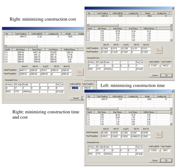
FIG. 10: Generated crew to minimize project time and cost TABLE 4: Generated crews for different optimization goals

Optimization Loader Truck Grader Compactor Time(hrs) Cost($) $/Q

992G 777D 24H 433E

Minimize Time 8 37 7 6 2580.99 39427467 12.2827

Minimize Cost 6 13 1 1 3441.32 16371000 5.1

Minimize Time & Cost

7 15 1 1 2949.7 16948800 5.28

Left: minimizing construction time

Right: minimizing construction time and cost

(15)

ITcon Vol. 12 (2007), Moselhi and Alshibani, pg. 135 2580.99 2949.7 3441.32 16371000 16948800 39427467 0 5000000 10000000 15000000 20000000 25000000 30000000 35000000 40000000 45000000 Cost 39427467 16948800 16371000 Time 2580.99 2949.7 3441.32 Time

FIG. 11: Optimization prototype output for the application example

6. SUMMARY AND CONCLUDING REMARKS

New methodology for optimization of crew formations for earthmoving operations has been presented. The developed methodology utilizes spatial technologies and genetic algorithm for optimization process. The methodology supports for: 1) optimum use of available resources, 2) track the involved equipment in near real time to improve the efficiency, productivity, and maximize contractor profit. The use of the GPS for data collection provides project teams with timely, inexpensive and accurate monitoring tool. Numerical example drawn from the literature to demonstrate the use and the capabilities of the developed methodology was analyzed.

7. APPENDIX A

void Main() { ga.setObjectiveType(MINIMIZE); ga.setSelectionType(USER_DEFINED_SELECTION, &mySelectionFunction); ga.setCrossoverType(USER_DEFINED_CROSSOVER, &myCrossoverFunction); ga.setPopulationSize(GeneticDlg.population); ga.setMaxNumberOfGenerations(GeneticDlg.m_MaxGeneration); ga.setUseElitism(true); ga.setSaveBestChromosome(true); ga.setCrossoverProbability(GeneticDlg.m_CrossOverPro); ga.setMutationProbability(GeneticDlg.m_MutationProbability); ga.setComputeStatisticsEvery(1); ga.setCheckForMatchingChromosome(true); // Display the statistics for the initial population ga.population().getMinimumFitness(); ga.population().getMaximumFitness(); ga.population().getAverageFitness(); ga.population().getStdDevFitness() ; // Run the genetic algorithm

ga.evolve(); ga.population().sort();

ga.population().writePopulationToFile("MyFile.txt"); // Display the overall best chromosome

for (i = 0; i < ga.bestChromosome().getNumberOfGenes(); i++) ga.bestChromosome().genes(i).getValue() ;

// Display the overall best chromosome fitness ga.bestChromosome().getFitness();

// Display the statistics for the final population ga.population().getMinimumFitness() ; ga.population().getMaximumFitness() ; ga.population().getAverageFitness() ;

(16)

ga.population().getStdDevFitness() ;

// Save the genetic algorithm statistics to a file. ga.writeStatisticsToFile("Stastic.txt");

ga.getNumberOfGenerations();

}

Chromosome & mySelectionFunction(Population &population) {

// Sort chromosomes from best to worst population.sort();

// Randomly choose chromosome within top 25% of the population int lastIndex = (int) (0.25f * (population.getNumberOfChromosomes() - 1)); return population.chromosomes(ga.randomInt(0, lastIndex));

}

void myCrossoverFunction(Chromosome &parent1, Chromosome &parent2, Chromosome *offspring1, Chromosome *offspring2) {

// If both offspring pointers are not null, create 2 offspring. Otherwise, create // only one offspring.

if (offspring1 && offspring2) {

// Create 2 offspring

for (int i = 0; i < parent1.getNumberOfGenes(); i++) { if (ga.flipBiasedCoin(0.5)) { offspring1->genes(i).setValue(parent1.genes(i).getValue()); offspring2->genes(i).setValue(parent2.genes(i).getValue()); } else { offspring1->genes(i).setValue(parent2.genes(i).getValue()); offspring2->genes(i).setValue(parent1.genes(i).getValue()); } } } else { // Create 1 offspring

for (int i = 0; i < parent1.getNumberOfGenes(); i++) { if (ga.flipBiasedCoin(0.5)) { offspring1->genes(i).setValue(parent1.genes(i).getValue()); } else { offspring1->genes(i).setValue(parent2.genes(i).getValue()); } } } }

void myMutationFunction(Chromosome &chromosome, int geneNumber) {

if (ga.geneDefinitions(geneNumber).geneType == INTEGER_GENE) {

// Integer Gene => Round Gaussian distributed random value before adding

chromosome.genes(geneNumber).setValue(chromosome.genes(geneNumber).getValue()+ roundFloat(ga.randomUnitGaussian())); }

else {

// Float Gene => Just add Gaussian distributed random value

chromosome.genes(geneNumber).setValue(chromosome.genes(geneNumber).getValue()+ ga.randomUnitGaussian()); } // Clip if necessary if (chromosome.genes(geneNumber).getValue() > ga.geneDefinitions(geneNumber).upperBound) chromosome.genes(geneNumber).setValue(ga.geneDefinitions(geneNumber).upperBound); if (chromosome.genes(geneNumber).getValue() < ga.geneDefinitions(geneNumber).lowerBound) chromosome.genes(geneNumber).setValue(ga.geneDefinitions(geneNumber).lowerBound); }

(17)

8. REFERENCES

AbouRizk M. and Hajjar D. (1998). A framework for applying simulation in construction, Canadian Journal of Civil Engineering, Vol. 25 No.3, 604–617.

Caterpillar, Inc. (1998). FPC users’ manual, Caterpillar Inc., Peoria, Ill.

Coley D. A. (1999). An introduction to genetic algorithm for scientists and engineers, World Scientific, River Edge, N.J.

Halpin W. and Woodhead W. (1976). Design of construction and process operations, John Wiley & Sons, Inc., New York.

Halpin D. and Riggs S. (1992). Planning and analysis of construction operations, John Wiley & Sons, Inc., New York.

Hassanien A. (2002). Planning and scheduling highway construction using GIS and dynamic programming, Ph.D. Thesis, Department of Building, Civil and Environmental Engineering, Concordia University, Montreal, Quebec.

Hassanien A. and Moselhi O. (2002). Automated data acquisition and planning of highway construction, Symposium on automation and robotics in construction, 19th (ISARC). Proceedings. National Institute of Standards and Technology, Gaithersburg, Maryland. September 23-25.

Holland H. (1992), Genetic algorithm, Sci. Am., July, 66–72.

John H., Michael V. and Julio M.(2005). Reduction of short-interval GPS data for construction operations analysis, Journal of Construction Engineering and Management 131(8) 920-927.

Kim J. (1989). An Object-oriented database management system approach to improve construction project planning and control, Ph.D. Thesis, University of Illinois, Urbana, Illinois.

Lothon A. and Akel S.(1996). Techniques for preventing accidental damage to pipelines, Proceedings of the 1st International Pipeline Conference(2), American Society of Mechanical Engineers, New York, NY, 643-650.

Marzouk M. and Moselhi O. (2000). Optimizing earthmoving operations using object-oriented simulation, In Proceedings of the 2000 Winter Simulation Conference, Orlando, Fla. Edited by J.A. Joines, R.R. Barton, P. Fishwick, and K. Kang. IEEE, Piscataway, N.J., pp.1926–1932.

Marzouk M. (2002). Optimizing earthmoving operations using computer simulation, Ph.D. Thesis, Department of Building, Civil and Environmental Engineering, Concordia University, Montreal, Quebec.

Oloufa A. (1993). Modeling operational activities in object-oriented simulation. Journal of Computing in Civil Engineering, Vol.7 No. 1, 94–106.

Oloufa A., Ikeda, M. and Hiroshi O. (2002).GPS-Based wirelesscollision detection of construction equipment, International Symposium on Automation and Robotics in Construction, 19th (ISARC). Proceedings. National Institute of Standards and Technology, Gaithersburg, Maryland. September 23-25, 2002, pp.461- 466.

Oglesby H., Parker W. and Howell A. (1989). Productivity improvement in construction, McGraw Hill Companies, New York, NY.

Reda R. (1990). Repetitive project modelling, Journal of Construction Engineering and Management, 116, No.2, 316-330.

Sacks R., Navon R., Shapira A. and Brodetzky I. (2002). Monitoring construction equipment for automated project performance control, International Symposium on Automation and Robotics in Construction, Stone, W. (ed.), Washington DC, September 2002. NIST SP 989, pp 161-166.