Optimization in semi-supervised classification of multivariate time series

(1)

Optimization in Semi-Supervised

Classication of Multivariate Time

Series

Pro Gradu Timo Lintonen 2192796 Research Unit of Mathematical Sciences University of Oulu Fall 2018

(2)

Nomenclature

List of Abbreviations

kNN k-nearest neighbor

Auslan Australian sign language

CBD-GA Class boundary detection using graphical analysis

CLeVer descriptive Common principal component Loading-based Vari-able subset selection method

CPC Common principal component

CPCA Common principal component analysis

DTW Dynamic time warping

ED Euclidean distance

EM Expectation maximization

i.i.d. Independent and identically distributed KKT Karush-Kuhn-Tucker (condition)

LOF Local outlier factor MTS Multivariate time series OCC One-class classication PCA Principal component analysis

PCA-SF Principal component analysis similarity factor PIP Perceptually important point

PU Positive-unlabelled (learning) RBF Radial basis function

RW Ratanamahatana-Wanichsan (criterion)

(5)

SSL Semi-supervised learning

SVC2004 The rst international signature verication contest SVDD Support vector data description

UTS Univariate time series Notations T _Transpose # Cardinality of a set s(k) State u(k) Action W(k) Random disturbance

X Matrix, time series

x Vector

X(j) One feature of a multivariate time series

λi Lagrangian multiplier for an inequality constraint

E Expected value

P Probability function

L Lagrangian function

X Time series database

µj Lagrangian multiplier for an equality constraint

µk Decision rule

∇ Gradient

π Policy

k · k Euclidean norm

e

(6)

ak

s(k)_→s(k+1) Transition cost

B(x, ) Ball with center x and radius D, dom Domain set and domain operator d(_·,_·) Distance function

d∗_{, p}∗ _{Dual and primal problem optimal values}

f, q Objective functions for primal and dual problems fk Function dening the system evolution

gi Function dening an inequality constraint

gk Cost functional

hj Function dening an equality constraint

J Dynamic programming cost function

m Number of dimensions

N Number of time series

n Number of observations, number of inequality constraints NU Number of unlabelled instances

S Set

ti Time stamp

Uk(s(k)₎ The set of admissible actions

W Warping path

x Scalar

a Ane hull

cl Closure

int Interior

relint Relative interior

(7)

Introduction

People are increasingly interested in monitoring their own lives. Some are interested in their blood pressure, some about the amount and quality of sleep they get and some about the daily consumption of calories. To ease their lives, people use embedded devices that monitor their surroundings using sensors.

In the every day business, there are many things to monitor. Shops record surveillance videos to aid in the ght against robberies. Steel producers mon-itor the quality of the steel. Investment bankers are interested in the prices of the stocks in the market.

One thing in common in all of these processes is that they produce time series type of data. Time series do not satisfy the assumption of the data points being independent and identically distributed (i.i.d.). Most models created for non-temporal data are build on this particular assumption. The vast number of sources of time series motivates us to study models that are able to process time series type of data.

The continuously expanding masses of data have created a demand for machine learning. Some tasks that have been automated successfully are classication and clustering. In many domains, these tasks can be automated to a degree that the automation increases business value drastically.

In this thesis, I will study the semi-supervised classication of multivari-ate time series. The main argument is that in semi-supervised time series classication the use of temporal models is justied over the non-temporal models. In Section 1 I will carefully go through the mathematics behind two successful algorithms: support vector data description and dynamic time warping. Section 1 is mostly based on the existing literature in the books [7] and [6]. In Section 2, the special characteristics of the time series are discussed, especially the distance calculations on time series. The Section 3 is dedicated to one-class classication and positive-unlabelled learning. In Section 4 I will test the models empirically on three time series datasets. Sections 5 and 6 conclude this thesis on observation of the results and the possible future research.

In this thesis, I will present a novel proof to Theorem 2.9 in Section 2.3.3 and a new method for semi-supervised learning of time series called Peak evaluation using perceptually important points in Section 3.4.3. In Section 2.3.3, I will also prove Lemmas 2.7 and 2.8 that are used in the proof to Theorem 2.9.

(8)

1 Optimization

Mathematical optimization is a eld that specializes in nding the optimal value of an objective function under some constraints. The optimum is the minimum value of a cost function or the maximum value of a utility func-tion. The optimum was dened as the minimum or the maximum already in the ancient Greek around 500 BC when the philosophers were interested in nding optima in elds such as physics, astronomy and the quality of human life and government [32].

In machine learning optimization is in an important role. Many models are made exible by introducing some hyper parameters. In some models these parameters may be chosen automatically to best t the data at hand. This is achieved, for example, by minimizing a loss function, such as least squares or log-loss.

In this thesis, two algorithms are presented that rely on optimization. The support vector data description is heavily based on convex programming. The dynamic time warping algorithm uses dynamic programming.

1.1 Non-linear Programming

Let us rst x the notation in the following denition.

Denition 1.1. Letf :X →RwithX ⊂Rmbe a function to be minimized. Then a non-linear program is

minimize

x_∈X f(x)

subject to gi(x)≤0, i= 1, . . . , n, hj(x) = 0, j = 1, . . . , p.

(1.1)

The function f is an objective function. The functions gi and hj dene

inequality constraints and equality constraints, respectively. There is also the constrain x _∈ X. This is called an abstract constraint. The constraints

dene a feasible region. That is the set of all the points satisfying all the con-straints. Throughout this thesis, the objective function f and the inequality

constraints dening functions g1, . . . , gn are assumed to be dierentiable.

The non-linear program in Equation (1.1) is dened over some domain. The domain of the optimization problem is a set in which the objective func-tion f and all the constraint functions gi and hi are dened. More formally,

the domain D of the program in Equation (1.1) is

D=dom f∩ n \ dom gi ! ∩ m \ dom hj ! . (1.2)

(9)

Historically, mathematical optimization has been divided into linear and non-linear programming. This thesis uses a modern, more meaningful division into convex and non-convex programming [50]. The next section is dedicated to convex programming.

1.1.1 Convex Programming

Convex programming holds many desirable properties. One of them is the fact that any locally optimal solution to a convex program is also global [50]. For example, the optimization of the k-means algorithm [23] minimizes

a non-convex objective function that has multiple local minima. Standard procedure when running a k-means algorithm is to run it multiple times

with dierent initial starting points. Even that, however, does not guarantee global optimum, and the result is usually a sub-optimal model.

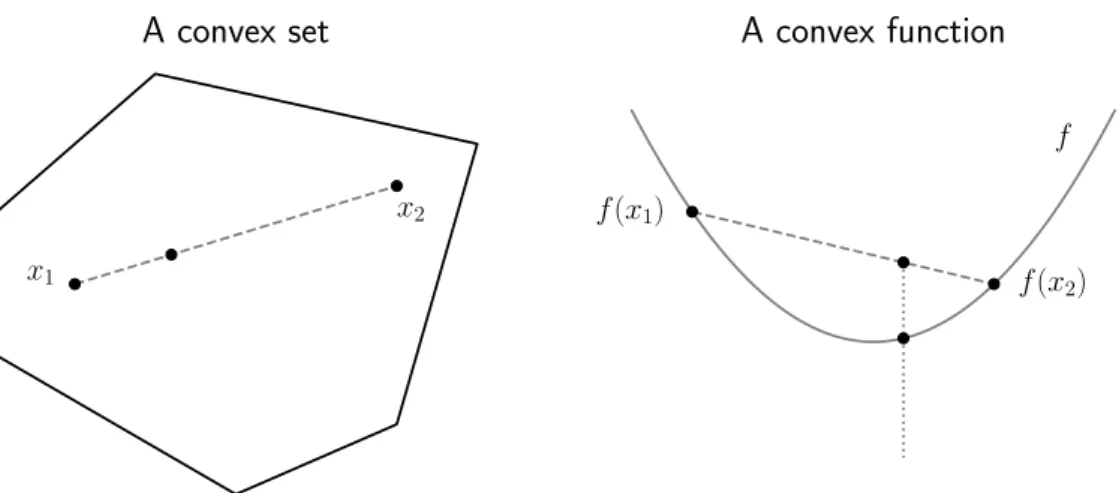
A convex program is a special case of the non-linear program in Denition 1.1. The two elementary concepts of convex programming are a convex set and a convex function. These concepts are illustrated in Figure 1. A set S is

convex if for any pair of points in the set S the convex combination of the

points is in the set S. More formally,

Denition 1.2. The set S is convex if tx1+ (1−t)x2 ∈S for all x1,x2 ∈S

and for all t∈[0,1].

There are two special cases to the convex sets. These are the empty set and the sets with only one element {x_{} ⊂}_Rm [50].

Denition 1.3. Let the set X ⊂ Rm be convex. A function f : X → R is convex if

f(tx1 + (1−t)x2)≤tf(x1) + (1−t)f(x2) (1.3)

for all x1,x1 ∈X and for all t ∈[0,1].

The link between a convex set and a convex function is that for any convex function g the set S ={x_∈_Rm _| g(x)≤0} is convex. Let x1,x2 ∈S. This

means that g(x1), g(x2)≤0. Then

g(tx1+ (1−t)x2)≤tg(x1) + (1−t)g(x2)≤t∗0 + (1−t)∗0 = 0. (1.4)

Thus, the point tx1+ (1−t)x2 ∈S.

Remark 1.4. A function may also be concave. The functionf in Denition 1.3

is concave if the inequality in Equation (1.3) holds with reversed direction such that f(tx1 + (1 − t)x2) ≥ tf(x1) + (1 −t)f(x2). It is easy to see

from the inequality in Equation (1.3) that if a function f is convex, then

the function −f is concave. The following example introduces a very special

(10)

x1 x2 A convex set f(x1) f(x2) f A convex function

Figure 1: Left: A convex set. The convex combination of any two points in the set belongs to the set. Right: A convex function. The convex combination of any two function values overestimates the true value of the function.

Example 1.5. A linear function is convex. Let c_∈_Rm. The linear function

L : X _→ _R is dened as L(x) = cT_x_{. Now, the value of the function} _L _in

the point tx1+ (1−t)x2 is

L(tx1+ (1−t)x2) = cT(tx1+ (1−t)x2) = tcTx1+ (1−t)cTx2

=tL(x1) + (1−t)L(x2).

(1.5)

As stated in Remark 1.4, linear function is also concave. This follows from the fact that the equality L(tx1+ (1−t)x2) =tL(x1) + (1−t)L(x2)satises

both inequalities in Equation (1.3) and the one in Remark 1.4.

Adding a constant and multiplying with a positive real number preserves the direction of an inequality. This means that adding any constant to a con-vex function or multiplying a concon-vex function with any positive real number results in a convex function. Also, a sum of two convex functions is a convex function as shown in the following example.

Example 1.6. A sum of any two convex functions is a convex function. Let the functions g : X1 → R and h : X2 → R be convex functions and let

f(x) =g(x)+h(x). Thenf(tx1+(1−t)x2) = g(tx1+(1−t)x2)+h(tx1+(1− t)x2) = tg(x1) + (1−t)g(x2) +th(x1) + (1−t)h(x2) =tf(x1) + (1−t)f(x2).

Example 1.7. A quadratic function f(x) = (1/2)xT_Qx₊_Ax is convex if

(11)

xTQx _≥0 for any x_∈_Rm. Examples 1.5 and 1.6 imply that it is sucient to show that the quadratic term is convex. Let g(x) = xT_Qx_{. Then}

g(tx1+ (1−t)x2) =(tx1+ (1−t)x2)TQ(tx1+ (1−t)x2) =t2_xT 1Qx1+ (1−t)2xT2Qx2+ 2t(1−t)xT1Qx2 =t[1−(1−t)]xT 1Qx1+ (1−t)(1−t)xT2Qx2 + 2t(1−t)xT 1Qx2 =txT₁Qx1+ (1−t)xT2Qx2 −t(1₋t)xT 1Qx1−t(1−t)xT2Qx2+ 2t(1−t)xT1Qx2 =tg(x1) + (1−t)g(x2)−t(1−t)(x1−x2)TQ(x1−x2) ≤tg(x1) + (1−t)g(x2) (1.6) since (x1 −x2)TQ(x1 −x2) ≥ 0 for a PSD matrix Q and t(1−t) ≥ 0 by

denition. Thus, the function g is convex, which means that the function f

is convex.

Lemma 1.8. The intersection of two convex sets, such that S=S1∩S2, is

a convex set.

Proof. Let x1,x2 ∈ S. Then x1,x2 ∈ S1 and x1,x2 ∈ S2 by the denition

of intersection. Let us assume that x = tx1+ (1−t)x2 ∈/ S for some t ∈

(0,1). Then, by the denition of intersection, x _∈/ S1 or x _∈/ S2. This is

a contradiction since the set S1 and S2 are convex sets. Thus, the set S is

convex.

Denition 1.9. The non-linear program in Equation (1.1) is convex if the objective function f is a convex function, and the feasible region is a convex

set.

The inequality constraintsgi(x)_≤0dene convex sets if the functionsgi

are convex. By Lemma 1.8, the intersection of these sets is a convex set. A set dened by an equality constraint hj(x) = 0 is a bit more restricted. The set Sj = _{x _∈ _Rm _| _hj_{(x) = 0}_} _{is convex if} _hj₍_t_x

1 + (1−t)x2) = 0 for all

x1,x2 ∈ Sj and t∈ [0,1]. One family of functions that satisfy this property

is ane functions. Ane function is a functionhj(x) = cTx+bwithc_∈_Rm and b _∈R. Now

hj(tx1+ (1−t)x2) = cT(tx1+ (1−t)x2) +b

=tcTx1+tb+ (1−t)cTx2+ (1−t)b

=thj(x1) + (1−t)hj(x2) = 0.

(1.7)

(12)

Corollary 1.10. The non-linear program in Equation (1.1) is convex if func-tions f and g1, . . . , gn are convex, and the function h1, . . . , hp are ane.

1.1.2 Karush-Kuhn-Tucker conditions

Kuhn and Tucker [34] rst published the necessary conditions for non-linear programming in 1951. Later these conditions became known as Karush-Kuhn-Tucker (KKT) conditions when it was revealed that Karush had stated these conditions in his master's thesis in1938. In 1959Slater [57] formulated the conditions under which the KKT conditions are also sucient. The def-initions and the proofs in this section are mainly from the book [7].

Let us consider the non-linear program in Equation (1.1). In this section, the non-linear program is not assumed to be convex since the KKT conditions can be derived to the non-convex programs, too. Let us rst study duality and then carry on to the KKT conditions. The non-linear program in Equation (1.1) has a Lagrangian function:

Denition 1.11. The Lagrangian function to the non-linear program in Equation (1.1) is L(x,λ,µ) = f(x) + n X i=1 λigi(x) + p X j=1 µjhj(x). (1.8)

The Lagrangian augments the objective function with the weighted con-straint functions. These weights,λi andµj, are called Lagrangian multipliers.

When considering duality, the non-linear program in Equation (1.1) is called a primal problem. The following denition denes a Lagrangian dual problem to the primal problem:

Denition 1.12. Lagrangian dual problem regarding the primal problem in Equation (1.1) is

maximize

λ0,µ_∈_Rp q(λ,µ) = infx∈XL(x,λ,µ). (1.9)

In this thesis, the relation λ0 is used as a shorter notation for λi _≥0 for alli= 1, . . . n. Let the point(λ∗,µ∗)be the point that maximizes the dual problem. Let d∗ _{be the value of the objective function of the dual problem}

at that point. Then

d∗ =q(λ∗,µ∗) = max

λ0,µ∈_Rpq(λ,µ) =_λmax₀_,_µ∈ Rp

inf

(13)

It is straightforward to see that the optimal value of the primal problem in Equation (1.1) has a similar form. The supremum of the Lagrangian subject to the point (λ,µ) is sup λ0,µ∈Rp L(x,λ,µ) = sup λ0,µ∈Rp " f(x) + n X i=1 λigi(x) + p X j=1 µjhj(x) # . (1.11)

The supremum in Equation (1.11) has a valuef(x)ifgi(x)≤0andhi(x) = 0 for all i= 1, . . . , n and j = 1, . . . , p. If these conditions are not satised, the

value is innite. Let the point x∗ be the point that optimizes the primal problem in Equation (1.1). Then the optimal value of the primal problem objective function is p∗ =f(x∗) = sup λ0,µ∈_RpL (x∗,λ,µ) = min x∈X_λsup₀_,_µ∈ Rp L(x,λ,µ) (1.12) because the pointx∗ must be in the feasible region. This means thatgi(x∗₎_≤

0 and hi(x∗_{) = 0} _{for all} _i_{= 1}_{, . . . , n}_and _j _{= 1}_{, . . . , p}_.

It is trivial that inf

x∈XL(x,λ,µ)≤ L(x,λ,µ)≤_λsup₀_,_µ∈_RpL(x,

λ,µ) (1.13) for allx_∈_Rn_,_λ₀_and_µ_∈

Rp. Especially this relation holds for minimum and maximum values such that

d∗ = max

λ0,µ∈_Rp_x∈inf_XL(x,λ,µ)≤min_x∈_X sup

λ0,µ∈Rp

L(x,λ,µ) =p∗. (1.14)

This property is called weak duality. Weak duality states that the optimal value of the dual problem in Equation (1.9) always lower bounds the optimal value of the primal problem in Equation (1.1). The dierence p∗₋_d∗ _{is called}

the duality gap, and it is always non-negative. In the special case when the property in Equation (1.14) holds with equality the duality gap vanishes. This case is called strong duality. In case of strong duality, the value d∗ _{is the}

best lower bound for the optimal value of the primal problem in Equation (1.1).

Let us assume that the strong duality holds. Then

f(x∗) = p∗ =d∗ =q(λ∗,µ∗) = inf x∈X f(x) + n X i=1 λ∗igi(x) + p X j=1 µ∗jhj(x) ! ≤f(x∗) + n X i=1 λ∗igi(x ∗ ) + p X j=1 µ∗jhj(x ∗ )≤f(x∗) (1.15)

(14)

because hj(x∗_{) = 0} _{for all}_j _{= 1}_{, . . . , p} _and _λ∗

igi(x∗)≤0 for alli = 1, . . . , n.

The latter inequality follows from the constraintsλ∗

i ≥0and gi(x

∗₎

≤0. The inequalities in Equation (1.15) can be replaced by equalities. This means that

λ∗

igi(x∗) = 0 for all i = 1, . . . , n because these terms must be non-negative.

This property is called complementary slackness. Let us consider the point (x∗_,_λ∗

,µ∗) _∈ Rm ×Rn×Rp where the point x∗ minimizes the primal problem in Equation (1.1), and the point (λ∗,µ∗) maximizes the dual problem in Equation (1.9). Let us also assume that the strong duality holds, such that f(x∗_{) =} _q_(λ∗

,µ∗). Since the point x∗ mini-mizes the Lagrangian L(x,λ∗,µ∗) over the variable x, the gradient must be zero at that point, such that ∇xL(x,λ∗,µ∗) = 0. Putting all this together,

one has derived Karush-Kuhn-Tucker (KKT) conditions:

Theorem 1.13 (Karush-Kuhn-Tucker condition). Let the point (x∗_,_λ∗

,µ∗) satisfy the strong duality. Then the point (x∗_,_λ∗

,µ∗) also satises the fol-lowing conditions: ∇f(x∗) + n X i=1 λ∗i∇gi(x ∗ ) + p X j=1 µ∗j∇hj(x ∗ ) = 0 _(1.16) gi(x∗)≤0 and hj(x∗) = 0 (1.17) λ∗ i ≥0 (1.18) λ∗_igi(x∗) = 0 (1.19) for all i= 1, . . . , n and j = 1, . . . , m.

Proof. The proof is in the derivation.

1.1.3 Slater's condition

In the previous section, it was shown that the strong duality ensures that the KKT conditions hold. The strong duality, however, does not hold generally even for convex programs. This is shown in the following example.

Example 1.14. Let us consider a minimization problem minimize

x_∈_R x

subject to x2 ≤0. (1.20)

This minimization problem is clearly a convex program. Its Lagrangian is

L(x, λ) =x+λx2. The objective function of the dual problem is the inmum

of the Lagrangian, such that q(λ) = infx∈R(x+λx

(15)

Let us assume thatλ >0. Now,x+λx2 _{is a parabola that opens upwards,}

and its minimum is at the root of its derivative. Let us set the derivative to zero such that Dx(x +λx2) = 1 + 2λx = 0. The derivative vanishes at x = −1/2λ so the parabola reaches its minimum at that point. Using this

information, the cost function of the dual problem is

q(λ) = inf x∈_R(x+λx 2 ) = − 1 2λ +λ − 1 2λ 2 =− 1 4λ. (1.21)

The function q has no maximum when λ _≥ 0. This means that the dual

problem has no solution. For this reason, d∗ _{is undened, and} _d∗ ₆₌_p∗_.

The problem of ensuring the strong duality, as demonstrated in Example 1.14, has lead to the study of constraint qualications. There are various constraint qualications that ensure strong duality. For convex programming, one such constraint qualication is Slater's condition. The Slater point and Slater's condition are dened later in this section in Denitions 1.17 and 1.18, respectively. These denitions use the denition of relative interior.

Denition 1.15. The relative interior of a set S _⊂Rm is

relint(S) =_{x_∈S _| B(x, )_∩a(S)_⊂S_} (1.22)

for some >0.

In Equation (1.22) the set B(x, ) :=_{x0 _∈Rm _{| k}_x0

−x_{k ≤}_} is a ball

with a center x and radius . The operator_{k · k} is the Euclidean norm.

Denition 1.16. Euclidean norm of a point x_∈Rm _is

kx_k:= (xTx)1/2 = v u u t m X i=1 xi2_. (1.23)

Also, in Equation (1.22) the set a(S) :={Pk

i=1αixi ∈Rm |αi ∈R, xi ∈ S, Pk

i=1αi = 1} is an ane hull of the set S for any k= 1,2, . . ..

Let us assume convexity from now on. Slater's condition is dened for a convex program.

Denition 1.17. Slater point is a point in the relative interior of the domain

D that satises gi(x)<0for all i= 1, . . . , n.

Denition 1.18 (Slater's Condition). The convex program in Equation (1.1) satises Slater's condition if there is a Slater point in its feasible region.

(16)

Before proving that Slater's condition implies strong duality for convex program, let us prove two helpful theorems: Supporting Hyperplane Theorem and Separating Hyperplane Theorem.

Theorem 1.19 (Supporting Hyperplane Theorem). Let the set S ⊂Rm be convex and non-empty. Let x¯ _∈/ int(S) be a point that is not in the interior of the set S. Then there is a hyperplane such that aT_x_¯ _≤_b _and _aT_s_≥_b _for

all s_∈S.

Proof. If the pointx¯ is not in the interior of the setS, then it is either outside

the closure of the set S or in the boundary of the set S. These two cases are

proven separately. Let us rst assume that x¯ ∈/ cl(S).

Let a pointxˆ _∈cl(S)be the projection of the pointx¯ to the set cl(S). In

other words, the inequality kxˆ ₋x¯_{k ≤ k}x₋x¯_k holds for all x _∈cl(S). Let us dene a= ˆx₋x¯ and b =aT_x_ˆ. The vector _a and the scalar _b will dene

the supporting hyperplane.

This rst case can be proven with a contradiction. Let us assume that the theorem does not hold for x¯ ∈/ cl(S). This means that there is some

x _∈ cl(S) with aTx < b. Because the set cl(S) is convex, there is a point xt=tx+ (1−t)ˆx∈cl(S)with allt∈[0,1]. It will be shown here that, with

some t suciently close to zero, the pointxt is closer to the point x¯ than its

projection xˆ. In other words, it will turn out that _kxt−x¯k < kxˆ−x¯k for

some t _∈[0,1].

The vectorxt−x¯ can be written as

xt−x¯ =tx+ (1−t)ˆx−x¯ = (ˆx−x) +¯ t(x−x) =ˆ a+t(x−x)ˆ . (1.24)

The squared norm of the vector xt−x¯ is then

kxt−x¯k2 =ka+t(x−x)ˆ k2 =aTa+t2 kx₋xˆ_k2+ 2taT(x₋x)ˆ =_kxˆ₋x¯_k2+t 2(aT_x −aTx) +ˆ t_kx₋xˆ_k . (1.25)

Here, the term aT_x ₋_aT_x_ˆ ₌ _aT_x ₋_{b <} ₀ by the assumption that the

theorem does not hold for x¯ ∈/ cl(S). Note that the term aTx₋aTxˆ does not depend on the variablet. When the multipliert is small enough, the term

2(aT_x₋_aT_x)+_ˆ _t_k_x₋_x_ˆ_k_<0. Then, from Equation (1.25), it can be seen that

kxt−x¯k< kxˆ −x¯k for some xt ∈cl(S). This inequality is a contradiction

since xˆ was selected so that _kxˆ ₋x¯_{k ≤ k}x ₋x¯_k for all x _∈ cl(S). This contradiction proves that aT_x_≥_b for all _x_∈cl(_S).

(17)

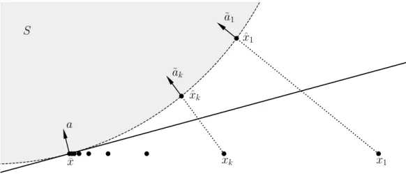
¯ x xk x1 ˆ xk ˆ x1 ˜ a1 ˜ ak a S

Figure 2: A visual proof of Supporting Hyperplane Theorem 1.19. The shaded area is a convex set. The normal vectors of the hyperplanes are the unit length vectors α˜k in the direction of the vectors xˆk−xk. This sequence of normal

vectors converges to the normal vectoraof the hyperplane that supports the convex set.

This sequence exists because x¯ ∈/ int(S). Let the projections of these points

to the set cl(S) be xˆk. From the previous part of this proof, it is known

that there exists a hyperplane such that aT

kx ≥ bk for all x ∈ cl(C) with

ak= ˆxk−xk and bk=aTkxk for all k = 1,2, . . .. Dividing by a positive real

number does not change the direction of the inequality, so the inequality

˜ aT_kx:= ak kxˆk−xkk T x_≥ bk kxˆk−xkk =: ˜bk (1.26)

holds for allx_∈cl(S). The vectora˜khas a normka˜kk= 1. This is illustrated

in Figure 2 where the arrows denote the vectors a˜k. Let us dene a :=

limk→∞a˜k and b :=aTx¯. Now the supporting hyperplane satises aTx≥ b

for all x_∈cl(S). Finally, the propositionaT_s_≥_bholds for all _s_∈_S because S ⊂cl(S).

Theorem 1.20 (Separating Hyperplane Theorem). Let the sets S1 and S2

be convex, non-empty, disjoint sets, such that S1 ∩S2 = ∅. Then there is a

hyperplane that separates them.

Proof. Let us dene a new set Y so that Y =_{u₋v _| u_∈S1, v _∈S2_}. Let

us rst show that this set is convex, and0∈/ Y. Then Supporting Hyperplane

(18)

The setY is convex because its elements are sums of elements from convex

sets. Also, 0 _∈/ Y. If it would be that 0 _∈ Y, then 0 =u₋v meaning that u =v. Thenu _∈S1 and u =v _∈S2 which is a contradiction since the sets S1 and S2 are disjoint.

From Theorem (1.19) it is known that there is a hyperplane such that aT₀_≤_band _aT_y_≥_b for all_y_∈_Y. This means that_aT_y_≥_aT₀= 0, which

implies thataT(u−v)≥0. From this result, it can be seen that the inequality

aT_u _≥ _aT_v _{holds for all} _u _∈ _S1 _and _v _∈ _S2_{. Especially this is true for the}

inmum and the supremum, which means that infu∈S1a

T_u _≥ _sup

v∈S2a

T_v.

This inequality proves the existence of the separating hyperplane.

Since the non-linear program is assumed to be convex, let us assume that the equality constraints dening functionhj are ane. These constraints can

be presented compactly as an equation (h1(x), . . . , hp(x))T ₌ _Ax₋_b ₌ ₀

with A _∈ _Rp×m and b _∈ _Rp. For the following proof, let us assume that rank(A) = p so the rows of Jacobian regarding the equality constraints are

linearly independent. If this condition is not satised, then either there are contradicting or unnecessary equality constraints [2].

Let us make another simplifying assumption that the set D has a

non-empty interior. This means that int(D) = _{x _∈ _Rm _| _B_(x_,₎ _⊂ _D_{} 6}₌ _∅

for some > 0. Then relint(D) = int(D). This assumption simplies the

following proof at the cost of some generality. The proof will, however, remain general enough for the rest of this thesis.

Theorem 1.21. Let relint(D) = int(D) and rank(A) = p. Then for this

convex program Slater's condition in Denition 1.18 implies strong duality. Proof. If the primal optimal solution is p∗ ₌ _−∞_{, then by weak duality}

the dual optimal solution is d∗

≤ p∗ ₌

−∞. This means that d∗ ₌ _p∗_{, and}

the proposition is always true. Let us next assume that the primal optimal solution is nite.

Let us rst dene two disjoint, convex sets

     A ={(u,v, t) |x_∈D, gi(x)≤ui, hj(x) =vj, f(x)≤t, i= 1, . . . n, j = 1, . . . p} B ={(0,0, s) |s < p∗_}_. (1.27)

Let us rst show that the sets A and B can be separated by a hyperplane.

This hyperplane will dene a useful relation between Lagrangian and the optimal primal value p∗_.

(19)

convex for a convex program. Let us study this proposition more carefully. Let us consider the point λ(u1,v1, t1) + (1₋λ)(u2,v2, t2) _∈ Rn+m+1 and points (u1,v1, t1),(u2,v2, t2) _{∈ A}. There are a point x1 that satises the

inequalities for (u1,v1, t1) and a point x2 that satises the inequalities for

(u2,v2, t2). Now

f(λx1+ (1−λ)x2)≤λf(x1) + (1−λ)f(x2)≤λt1+ (1−λ)t2 (1.28)

for any λ_∈[0,1]because of the convexity of the function f. The functions gi

are convex and the functions hj are ane and thus behave similarly to the

functionf. This means that the pointλx1+(1−λ)x2 satises the inequalities

for the point λ(u1,v1, t1) + (1₋λ)(u2,v2, t2) for all λ_∈[0,1] and the set_A is indeed convex.

The sets A and B do not intersect. If they did, there would be a point

(0,0, t) _∈ Rn+m+1 belonging in both sets A and B. If the point (0,0, t) belongs to the set A, there exists a pointx_∈D that satises all the primal

constraintsgi(x)≤0andhi(x) = 0. In addition, the objective function value

at the point x has an upper bound f(x) _≤ t. If the point (0,0, t) belongs to the set B too, the upper bound t satises the inequality t < p∗_{. This is a}

contradiction since p∗ _{is the optimal primal solution. Thus, the sets} _A _and

B must be disjoint.

Now that the sets A and B are shown to be convex and disjoint, let us

use Separating Hyperplane Theorem 1.20 on them. Separating Hyperplane Theorem 1.20 states that there exist a vector(˜λ,ν˜, µ)₆=0and a scalarα_∈_R

satisfying the following inequalities:

(˜λ,ν˜, µ)T(u,v, t)≥α (1.29)

for all (u,v, t)_{∈ A} and

(˜λ,ν˜, µ)T(0,0, s)≤α (1.30)

for all (0,0, s)_{∈ B}.

Equation (1.29) implies that _λ˜ ₀ _and _µ _≥ _{0. If any component} in the vector _λ˜ _{or the scalar} _µ _{were negative, the corresponding} compo-nent in (u,v, t) could be arbitrarily large and still (u,v, t) _{∈ A}. In other words, for any α ∈ R there would be either ui or t with both (u,v, t) ∈

A and (˜λ,ν˜, µ)T_(u_,_v_{, t}₎ _{< α}_{. This would mean that the inner product}

(˜λ,ν˜, µ)T_(u_,_v_{, t}₎would not be bounded from below. This contradicts

Equa-tion (1.29) and proves that_λ˜ ₀ _and_µ_≥_{0. Now there are two cases: either}

µ > 0or µ= 0. Let us rst prove that µ >0 implies strong duality.

Equation (1.30) implies thatµs_≤α. This is true for alls < p∗_{. Especially}

this relation holds for the supremum of the scalar s. From Equation (1.27),

it can be seen that sups=p∗_{. This means that} _µ_(sup_s_{) =}_µp∗

(20)

For anyx_∈D, there is a point(g1(x), . . . , gn(x), h1(x), . . . , hp(x), f(x))

∈ A. From this and Equations (1.29) and (1.30), one can see that

n X i=1 ˜ λigi(x) + p X j=1 ˜ νjhj(x) +µf(x)_≥α_≥µp∗ (1.31) for any x_∈D.

Let us divide Equation (1.31) by µ. This can be done since µ > 0 by assumption. This results in the following equation

n X i=1 ˜ λi µgi(x) + p X j=1 ˜ νj µhj(x) +f(x) = L(x,λ˜/µ,ν˜/µ)≥p ∗ _(1.32)

which holds for allx_∈D. Taking the inmum overxof the Lagrangian in the inequality in Equation (1.32) results in inequality infx∈DL(x,λ˜/µ,ν˜/µ) = q(˜λ/µ,ν˜/µ) _≥ p∗_{. By weak duality} _q_(˜_λ_/µ,_ν˜_/µ₎

≤ p∗_{. This means that}

p∗ ₌_q_(˜_λ_/µ,_ν˜_/µ_{) =} _d∗_{. In other words, strong duality holds if} _{µ >}_0.

Let us now show thatµ is positive when Slater's condition holds. Let us

consider the second case where µ = 0. This selection will lead to a contra-diction. Now Equation (1.31) implies that

n X i=1 ˜ λigi(x) + p X j=1 ˜ νjhj(x)≥0 (1.33)

for all x _∈ D. Especially Equation (1.33) holds for the Slater point x˜. In addition, the Slater point satises the equality constraints, so

n

X

i=1

˜

λigi(˜x)≥0. (1.34)

Since for the Slater point gi(˜x) < 0 for all i = 1, . . . n, the left side of the

inequality in Equation (1.34) can have non-negative value only if _λ˜ ₌ ₀_. Note that Separating Hyperplane Theorem (1.20) implies that (˜λ,ν˜, µ)₆=0.

Since µ= 0 and λ˜ =0, the only possibility left is thatν˜ ₆=0.

Let us now show that the property ν˜ ₆= 0 cannot hold. Since µ = 0 and ˜

λ=0, the inequality in Equation (1.33) implies that

p

X

j=1

˜

(21)

for all x _∈ D assuming that the function hj are ane. The Slater point

satises the equation

p

X

j=1

˜

νjhj(˜x) = ˜νT(Ax˜₋b) = 0 (1.36)

by denition. The Slater point is in the interior of the domain D, such that

˜

x_∈int(D). This means that there exists at least onex_∈Dthat satises the

inequalityν˜T(Ax−b)<0unlessATν˜ =0. However, the equationATν˜ =0

cannot hold for rank(A) =p and ν˜ ₆=0. From this it can be concluded that

˜

ν = 0. This means that the identity (˜λ,ν˜, µ) _≡ 0 holds, which contradicts

Separating Hyperplane Theorem 1.20. This contradiction followed from the assumptionµ= 0. Since µis non-negative, the only possibility is thatµ >0, which was proven earlier in this proof.

Let us summarize this section. Let the non-linear program in Equation (1.1) be convex. Let it also satisfy the Slater's condition in Denition 1.18. Then there exists at least one point (x∗_,_λ∗

,µ∗) that satises strong duality. These points, which satisfy strong duality, also satisfy KKT conditions in Theorem 1.13. In addition, the variable x∗ in any of those points is the global optimum to the primal problem in Equation (1.1).

1.2 Dynamic Programming

In the previous section, the minimization involved only one decision: the optimal selection of the point x∗. This section is dedicated to the systems that involve multiple decision to be made over time. These systems are called dynamic. The main reference in this section is [6].

1.2.1 Discrete-time Dynamic System

time dynamic system is a system that evolves with time. Discrete-time refers to that the system changes its state every once in a while. Let the state of the system at time k be s(k) _∈ Sk. A state change is observed

at times k = 0,1, . . . , K. These time instants constitute a planning horizon.

The value K is called the end of the planning horizon. These notations are

used to formally dene the discrete-time dynamic system.

Denition 1.22 (Discrete-time dynamic system). Let the state s(0) _∈ S0

be a xed rst state in a planning horizon k = 0,1, . . . , K. For the

fol-lowing time points, the system evolves according to a function s(k+1) ₌ fk(s(k)_,_u(k)_,_W(k)

) where u(k)_∈Uk(s(k)₎_{is an action taken, and} _W(k)

∈Dk

(22)

Let us assume that the random disturbances W(k) are independent of each other. The domain Uk(s(k)₎ _{is a set of actions that are allowed at the}

current state. At each time point k, an action is chosen from the domain Uk(s(k)_{). The selection is done based on a rule:}

Denition 1.23. Function µk is a decision rule. It makes a decision based

on the knowledge of the current state, and it realizes as an action such that u(k) =µk(s(k)_).

Decision rules constitute a policy:

Denition 1.24. A policy π = (µ0, µ1, . . . , µK−1) is a sequence of decision

rules selected over the planning horizon.

A policy is a sequence of functions. The policy determines which action to take at any time at any state. This means that the policy selected will generate an action depending on the current state. The goal of dynamic programming is to nd the optimal policy. The optimal policy will determine the optimal actions in any state.

The value of the policy is measured by an objective function. In this section, the objective is to minimize a cost function. One characteristic of dynamic programming is that the cost function consists of multiple cost func-tionals. Let function gk be a cost functional, a function of the current state,

the action taken and a random disturbance. Its value is gk(s(k)_,_u(k)_,_W(k)

) for k= 0,1, . . . , K₋1 andgK(s(K)₎_{. Now, nding the optimal policy can be}

stated as a dynamic program:

Denition 1.25. Let the system in Denition 1.22 evolve according the func-tions fk, and let the costs of the states, actions and random disturbances

oc-cur according the cost functionalsgkover a planning horizonk = 0,1, . . . , K.

Then the dynamic program is

minimize π_∈Π Jπ(s (0)_{) =} E " gK(s(K)_{) +} K−1 X k=1 gk(s(k)_{, µk}_(s(k)₎_,_W(k) ) # subject to s(k+1) =fk(s(k)_{, µk}_(s(k)₎_,_W(k)₎ _{, k} _{= 0}_{, . . . K} −1. (1.37)

The domainΠ is a set of all admissible policies. For an admissible policy, all decisions yield an action that is allowed in the current state, such that

µk(s(k)₎ _∈ _Uk_(s(k)₎_{. The symbol}

E means expected value over all random vectors W(0),W(1), . . . ,W(K−1).

(23)

Deni-Denition 1.26. Let the dynamic program be dened as in Deni-Denition 1.25. Its sub-problem over a planning horizon l=k, . . . , K is

minimize πk∈Πk Jπk(s (k)_{) =} E " gK(s(K)_{) +} K−1 X l=k gl(s(l)_{, µl}_(s(l)₎_,_W(l) ) # subject to s(l+1) =fl(s(l)_{, µl}_(s(l)₎_,_W(l)₎ _{, l}₌_{k, . . . K} −1 (1.38)

In Equation (1.38), the policy πk = (µk, . . . , µK−1) is a truncated policy.

The existence of sub-problems is another characteristic for dynamic program-ming. The following section will show that a dynamic program may be solved by breaking it down into easier sub-problems and solving them in succession. This is possible because of the principle of optimality [5]. The following sec-tion is dedicated on the study of that principle.

1.2.2 Bellman's principle of optimality

In 1957, Bellman stated the often quoted principle of optimality: The Principle of Optimality. An optimal policy has the property that whatever the initial state and initial decisions are, the re-maining decisions must constitute an optimal policy with regard to the state resulting from the rst decision. [5, p. 83]

This rather general denition is expressed more formally using Denitions 1.25 and 1.26 in the following statement: If the policyπ∗ _{= (}_µ∗

0, µ∗1, . . . , µ∗K−1)

is an optimal policy for the dynamic programming problem in Equation (1.37), then the policy π∗

k = (µ

∗

k, . . . , µ

∗

K−1) is an optimal policy for the

dynamic programming sub-problem in Equation (1.38) [6]. This means that the problem in Equation (1.37) has an optimal substructure.

Let us use a shorter notation for the cost function of the sub-problem denoted asJk(s(k)_{) :=}_Jπk_(s(k)₎from now on. Let us use a similar notation for

the optimal solution to the sub-problem too, denoted asJ∗

k(s(k)) :=Jπ∗k(s (k)_).

The following theorem states the principle of optimality formally.

Theorem 1.27 (Bellman's principle of optimality). Let the policy π∗ ₌

(µ∗

0, µ∗1, . . . , µ∗K−1) minimize the problem in Equation (1.37). Then the

trun-cated policyπ∗ k = (µ ∗ k, µ ∗ k+1, . . . , µ ∗

K−1)minimizes the sub-problem in Equation

(1.38).

Proof. This theorem is proven for nite planning horizon k = 1, . . . , K and

(24)

means that Jπ∗(s(0)) ≤ Jπ0(s(0)) for all π0 ∈ Π. Let us prove this theorem

using a contradiction. Let us assume that the policy π∗

k is a sub-optimal

policy for sub-problem in Equation (1.38). The sub-optimality of the policyπ∗

k

means that there exists some policy π0

k = (µ0k, . . . , µ0K−1)∈ Πk that satises the inequality Jπ0 k(s (k)₎ ≤Jπ∗ k(s (k)₎ _(1.39)

for all possible states s(k) _∈_Sk. In addition, the strict inequality in Equation

(1.39) holds for at least one state s(k) that occurs with positive probability. This assumption will lead to a contradiction.

Let p(w(i)_,_w(j)₎ denote the joint probability. The joint probability is

dened as p(w(i)_,_w(j)_{) :=}

P(W(i) = w(i) ∩ W(j) = w(j)). Because the disturbances are independent of each other, the equality p(w(i)_,_w(j)_{) =} p(w(i)₎_p_(w(j)₎ holds for all _{i, j} _{= 0}_,₁_{, . . . , K} ₋₁ where _i ₆₌ _j and for all

w(i) _∈Di,w(j) _∈Dj.

The state s(k+1) _{is a random vector that is dependent on} _W(k)_{. This}

follows from the evolution of the system s(k+1) ₌ _fk_(s(k)_,_u(k)_,_W(k)_{). By}

recursion, this means that the value of a cost functional gk(s(k)_,_u(k)_,_W(k)

) depends on the previous random disturbances W(0), . . . ,W(k). On the other hand, the value of the cost functional gk(s(k)_,_u(k)_,_W(k)

) does not depend on any future disturbance W(l) for k < l as the random disturbances are

independent of each other. This means that the expected value of the cost functional is EW(l)gk(s(k),u(k),W(k)) = gk(s(k),u(k),W(k))

P

w(l)p(w(l)) =

gk(s(k)_,_u(k)_,_W(k)₎ _{for all} _{k < l}_.

The value of the dynamic programming cost function for the optimal policy π∗ is Jπ∗(s(0)) = _E W(0)_,...,_W(K−1) " gK(s(K)_{) +} K−1 X l=0 gk(s(l)_{, µ}∗ l(s(l)),W (l) ) # = X w(0)_,...,_w(K−1) p(w(0)₎_{, . . . , p}_(w(K−1)₎ " gK(s(K)₎ + K−1 X l=0 gk(s(l), µ∗l(s (l) ),w(l)) # . (1.40)

The second equality in Equation (1.40) follows from the independence of the random disturbances. Since the values of the cost functionals are independent of future disturbances, the right side of Equation (1.40) can be computed in

(25)

pieces such as Jπ∗(s(0)) = X w(0)_,...,_w(k−1) p(w(0)₎_{, . . . , p}_(w(k−1)₎ "_k₋₁ X l=0 gl(s(l)_{, µ}∗ l(s (l)₎_,_w(l)₎ + X w(k)_,...,_w(K−1) p(w(k)₎_{, . . . , p}_(w(K−1)₎ gK(s(K)₎ + K−1 X l=k gl(s(l)_{, µ}∗ l(s(l)),w(l)) # . (1.41) Again, using the assumption of independent disturbances, Equation (1.41) can be rewritten using expected values. Then the nested expected value is nothing else than the optimal value of the sub-problem in Equation (1.38). Now the optimal value may be written using the sub-problem value such that

Jπ∗(s(0)) = _E W(0)_,...,_W(k−1) "_k₋₁ X l=0 gl(s(l)_{, µ}∗ l(s (l)₎_,_W(l)₎ + E W(k),...,W(K−1) gK(s(K)_{) +} K−1 X l=k gl(s(l)_{, µ}∗ l(s (l)₎_,_W(l)₎ # = E W(0)_,...,_W(k−1) "_k₋₁ X l=0 gl(s(l), µ∗l(s (l) ),W(l)) +Jπ∗ k(s (k) ) # . (1.42)

Using the linearity of the expected value, the following inequality holds:

Jπ∗(s(0)) = E W(0),...,W(k−1) "_k₋₁ X l=0 gl(s(l), µ∗l(s (l) ),W(l)) # + E W(0),...,W(k−1) Jπ∗ k(s (k) ) > E W(0)_,...,_W(k−1) "_k₋₁ X l=0 gl(s(l)_{, µ}∗ l(s (l)₎_,_W(l)₎ # + E W(0)_,...,_W(k−1)Jπ 0 k(s (k)₎_. (1.43) The last inequality is strict since there is at least one state s(k) that

corre-sponds to a probability p(w(0)_{, . . . ,}_w(k−1)₎ _> ₀ _with _Jπ₀ k(s

(k)₎ _{< Jπ}_∗ k(s

(k)_).

This follows from the assumption of the policy π∗

k being sub-optimal. From

Equation (1.43), it can be see that the policy

πl _{= (}_µ∗ 0, . . . , µ ∗ k−1, µ 0 k, . . . , µ 0 K−1) (1.44)

(26)

results in a lower over all cost function value Jπl(s(0)) < Jπ∗(s(0)). This is

a contradiction, since the policy π∗ _{is optimal policy. This proves Bellman's}

principle of optimality.

Bellman's principle of optimality makes it possible to divide the dynamic program in Equation (1.37) into sub-problems. The reasoning behind this is that if the sub-problems are not solved optimally, then the solution to the dynamic program cannot be optimal. This strategy ecient because each sub-problem is a dynamic program. This means that the sub-problems may be divided further by using Bellman's principle of optimality. This recursion can then be used until solving the sub-problems becomes trivial. This idea is presented formally in Algorithm 1.

Algorithm 1 Backward Dynamic Programming Algorithm 1: JK(s(K)_{) =}_gK₍_s(K)₎ 2: for all k =K₋1, . . . ,1,0 do 3: Jk(s(k)₎ ₌ _min u(k)_∈_Uk(_s(k)₎_E_W(k)[gk(s(k),u(k),W(k)) + Jk+1(fk(s(k)_,_u(k)_,_W(k) ))] 4: end for

Algorithm 1 starts by solving the trivial problems JK(s(K)_{). These}

re-sults are then used to solve the preceding sub-problems. The following theo-rem proves that Algorithm 1 yields an optimal solution, which is J∗

k(s(k)) = Jk(s(k)_).

Theorem 1.28. Let the random disturbances come from domains Dk that

are nite or countable. Let E[gk(s(k), µk(s(k)),w(k))] < ∞ for all admissi-ble policies πk = (µk, . . . , µK) with decision rules µk(s(k)₎ _∈ _Uk_(s(k)_{). Then}

the value Jk(s(k)₎ _{in Algorithm 1 is the optimal cost function value for the}

program in Equation 1.38. Let u(k)∗ be the solution to the _kth minimization

problem in Algorithm 1. If there exist optimal decisions satisfying identity u(k)∗ _≡ _µ∗ k(s(k)), then π ∗ _{= (}_µ∗ 0, µ ∗ 1, . . . , µ ∗

K−1) is the optimal policy to the

program in Equation 1.37.

Proof. Theorem 1.28 is proven by using induction. The case where k =

K is trivial since there is no action to take. It means that JπK(s(K)_{) =}

E[gK(s(K))] = gK(s(K)) with the optimal policy being πK = ∅. Let us now consider the cases where k < K.

Let us assume that the Algorithm 1 gives an optimal solution for some

k + 1. In other words, let Jk+1(s(k+1)_{) =} _J∗

(27)

optimal value J∗

k(s(k)) for the sub-problem in Equation (1.38) is J_k∗(s(k)_{) =} _min (µk,πk+1)∈Πk E " gK(s(K)_{) +} K−1 X l=k gl(s(l)_{, µl}_(s(l)₎_,_W(l)₎ # (1.45)

by Denition 1.26. In Equation (1.45), a shorter notation is used for the policy (µk, πk+1) := (µk, µk+1, . . . , µK−1) =πk. This shorter notation highlights the

relation between the cost functions Jπk and Jπk+1 that are the cost functions of the successive sub-problems.

Let us use Bellman's principle of optimality to Equation (1.45): If the policy (µ∗

k, π

∗

k+1) minimizes the cost function Jπk(s(k)), then the policyπ

∗

k+1

minimizes the cost function Jπk+1(s

(k)). This means that

Jk∗(s (k) ) = min µk _WE(k) " gk(s(k), µk(s(k)),W(k)) + min πk+1∈Πk+1 E W(k+1),...,W(K−1) gK(s(K)₎ + K−1 X l=k+1 gl(s(l)_{, µl}_(s(l)₎_,_W(l) ) # = min µk _WE(k) h gk(s(k), µk(s(k)),W(k)) +Jk+1∗ (s (k+1) )i (1.46)

where µk(s(k)₎ _∈ _Uk_(s(k)_{). In Equation (1.46), the state at the time} _k _{+ 1}

can be written as s(k+1) ₌ _fk_(s(k)_,_u(k)_,_W(k)₎_{. Then, for any state} _s(k)_{, the}

expression on the right side of Equation (1.46) is minimized by minimiz-ing over the action u(k). Now, by the induction assumption Jk+1(s(k+1)_{) =} J∗

k+1(s(k+1)), the equation in Step 3 of Algorithm 1 holds since J_k∗(s(k)_{) =} _min uk∈Uk(s(k)) E W(k) h gk(s(k)_,_u(k)_,_W(k)_{) +}_Jk+1₍_fk_(s(k)_,_u(k)_,_W(k)₎₎i =Jk(s(k)₎_. (1.47) Thus, by induction, Algorithm 1 gives the optimal solution at each index k

such that Jk(s(k)_{) =} _J∗

k(s(k)).

1.2.3 Deterministic discrete-time dynamic system

Deterministic discrete-time dynamic system is a special case of the system presented in Denition 1.22. In the absence of the disturbance, the discrete-time dynamic system is deterministic. This means that the next state is

(28)

determined fully by the current state and the action taken, such as s(k+1)=

fk(s(k)_,_u(k)₎_{. In this case, the cost functional is xed on a xed state and}

a xed action. Instead of the cost functional, a transition cost is used. The transition cost is dened as ak

s(k)_→s(k+1) = gk(s

(k)_,_u(k)₎ _with _u(k) _∈ _Uk_(s(k)₎

for all k= 0,1, . . . , K ₋1and aK

s(K)_→s(K+1) =gk(s

(K)₎_.

To be precise, the transition cost is not well dened if two dierent actions on a same state result in a same successive state s(k+1) = fk(s(k)_,_u(k)_{) =} fk(s(k)_,_v(k)₎ _{for some} _u(k)_,_v(k) _∈ _Uk_(s(k)₎ _with _u(k) ₆₌ _v(k)_{. In these cases,}

let us selectak

s(k)_→s(k+1) = min{gk(s(k),u(k)), gk(s(k),v(k))}because the higher cost could never be in the optimal solution.

For completeness, let us set transition costs for illegal transitions and self-transitions, too. Let ak

s(k)_→s(k+1) = ∞ for illegal transitions with the state changes(k+1) =fk(s(k)_,_u(k)₎_where_u(k)_∈_/ _Uk_(s(k)_{). For self-transitions,} ak

s(k)_→s(k+1) = 0 with the state change s(k) = s(k+1). Both denitions apply for all k = 0,1, . . . , K −1. Now, the complete denition for the transition

cost is ak_s(k)_→s(k+1) =      0 , if s(k) ₌_s(k+1) gk(s(k)_,_u(k)₎ _{, if} _u(k)_∈_Uk_(s(k)₎ ∞ , otherwise. (1.48)

Using the transition cost notation instead of the cost functionals, cost func-tion J can be written as

Jπ(s(0)_{) =} E W(0)_,...,_W(K−1)[gK(s (K)_{) +} K−1 X k=0 gk(s(k)_{, µk}_(s(k)_))] =gK(s(K)_{) +} K−1 X k=0 gk(s(k)_{, µk}_(s(k)₎₎ =aK_s(K)_→s(K+1) + K−1 X k=0 ak_s(k)_→s(k+1). (1.49)

The expected value over the random disturbances in Equation (1.49) can also be removed because in a deterministic system, the cost functionals do not depend on any random disturbances.

Knowing the transition costs ak

s(k)_→s(k+1), nding the optimal policy is a

minimization problem, or more specically, a shortest path problem:

Denition 1.29. Let the transition costs be dened as in Equation (1.48). Then the shortest path problem is

(29)

minimize (s(0)_{, . . . ,}_s(K)₎ Jπ(s (0)_{) =}_aK s(K)_→s(K+1) + K−1 X k=0 ak s(k)_→s(k+1). (1.50) The shortest path problem in Denition 1.29 may be solved recursively using backward dynamic programming algorithm:

     JK(s(K)_{) =}_gK_(s(K)_{) =} _aK s(K)_→s(K+1) Jk(s(k)₎ _{= min[}_gk_(s(k)_,_u(k)_{) +}_Jk+1_(s(k+1)_)] = min[ak s(k)_→s(k+1)+Jk+1(s (k+1)_)] (1.51)

with an optimal solution J0(s(0)_{) = min[}_a0

s(0)_→s(1) +J1(s

(1)_)]_.

Remark 1.30. Theorem 1.28 requires the cost functional valuesgk(x(k)_,_u(k)₎

to be nite. In this section, however, the transition costs are dened to be innite for illegal transitions. This denition was chosen only to keep the notation more simple. For the same results, the transition costs do not need to be innite for illegal transitions. A large enough value M would suce.

Let the constant M be remarkably greater than the sum of all the legal

transitions, dened as PK−1 k=0 P s(k)_∈_Sk P u(k)_∈_Uk(_s(k)₎gk(s(k),u(k))M <∞. Let the transition cost be ak

s(k)_→s(k+1) = M for illegal transitions where s(k+1) = fk(s(k)_,_u(k)₎ _and _u(k) _∈_/ _Uk_(s(k)_{). Now the algorithm in Equation}

(1.51) would never pick an illegal transition if there is a legal transition avail-able. Also, if J0(s(0)₎ _≥ _M, it means that no admissible policy exists. With

this remark in mind, the solution in Equation (1.51) is can be seen as optimal by Theorem 1.28.

Since there are no disturbances, and every state can be calculated from the actions taken, the shortest path problem may be reversed. In a reversed problem, the state s(0) is the nal state, and the ctitious state s(K+1) is the rst state of the system. Let us dene transition costs as aK−k

s(k+1)_→s(k) :=

ak

s(k)_→s(k+1). These are the costs for reversed transitions, and they are equal

to the original, non-reversed costs. Let us also dene states t(k) _:=_s(K−k+1)_,

which means thats(l) ₌_t(K−l+1). The reversed shortest path problem is

minimize (s(1)_{, . . . ,}_s(K+1)₎ e Jπ(s(K+1)_{) =}_aK s(1)_→s(0)+ K X k=1 aK−k s(k+1)_→s(k), (1.52) which is equivalent to

(30)

minimize (t(0), . . . ,t(K)) e Jπ(t(0)_{) =}_aK t(K)_→t(K+1) + K−1 X k=0 ak t(k)_→t(k+1). (1.53) The minimization problem in Equation (1.53) has been solved in Equation (1.51). When the replacementt(k) ₌_sK−k+1 _{is used, the result is the forward}

dynamic programming algorithm.

     e JK(s(1)₎ ₌_aK s(1)_→s(0) =a0_s(0)_→s(1) e Jk(s(K−k+1)_{) = min[}_ak s(K−k+1)_→s(K−k) +Jk+1e (s(K−k))] = min[aK−k s(K−k)_→s(K−k+1) +Jk+1e (s (K−k)_)] (1.54)

with an optimal solution J0e(s(K+1)) = min[aK

s(K)_→s(K+1) +J1(s

(K)_{)]. This}

al-gorithm is presented formally in Alal-gorithm 2.

Algorithm 2 forward dynamic programming algorithm 1: JKe (s(1)) =a0_s(0)_→s(1) 2: for all k =K₋1, . . . ,1,0 do 3: Jke(s(K−k+1)) = min_s(K−k)[aK−k s(K−k)_→s(K−k+1)+Jk+1e (s(K−k))] 4: end for

2 Time Series

Time series are a sequence of observations made over time. Some examples of time series are market capitalization indices, such as S&P 500, electrocar-diograph and audio les. Ding et al. [17] dene time series in discrete time as a set of pairs of time stamps and observations.

Denition 2.1. Let xi _∈ R be an observation that occurs at time ti. Time series is a set of pairs T ={(xi, ti)}n

(i=1) with ti < tj for all i < j.

The time series T is a sample from some continuous signal. Usually, the sampling rate is assumed to be xed [19, 24, 71], so that ∆ti := ti ₋ti−1

is constant for all i. In these cases the time stamp is usually irrelevant and

may be dropped. With this assumption, the time series has the following representation:

(31)

se-The series X dened this way is called a univariate time series (UTS). A data point xi is usually called a feature or a dimension. In this thesis,

however, it is called an observation or a dimension to avoid confusion when talking about feature subset selection in section 2.2.

There may be multiple simultaneous measurements for capturing dierent aspects of a single event. This kind of arrangement creates multiple time series that are logically connected by the event. These time series can be processed as one multivariate time series (MTS). MTS are dened using the denition of UTS in Denition 2.2:

Denition 2.3. Multivariate time series is a collection of univariate time series X = (X(1)_{, . . . ,}_X(m)₎ _with _X(j) _{being a univariate time series of}

length n for all j = 1, . . . , m.

In this thesis, the UTS X(j) in Denition 2.3 is called a feature of the MTS. The MTS in Denition 2.3 may also be presented as a matrix X _∈ Rn∗m. It is also possible to present it as a sequence of multivariate observa-tions X = (x1, . . . ,xn)similarly to Denition 2.2.

Classication of time series data poses multiple challenges. First, time series may have dierent lengths. This means that the vectors to be compared may be of dierent dimension. Second, if MTSs consist of multiple features, classication may suer from so-called curse of dimensionality [18]. Third, time series are collections of observations that are usually highly correlated to the previous and subsequent observations. This means that there are multiple ways to dene distance between time series. Some distances represent the dierence between time series well, while other distances may not.

The following sections will review some of the methods to tackle these challenges. Section 2.1 is about preprocessing of time series. Section 2.2 presents methods to reduce the number of features to tackle the curse of dimensionality. In section 2.3, some commonly used distance measures to compare the time series are discussed.

2.1 Preprocessing of time series data

There are two preprocessing steps that the time series generally require: resampling andZ-normalization. Resampling transforms the time series into

desired length [48].Z-normalization eliminates the scale and oset dierences

between the time series [4]. Both of these methods are designed for UTSs. They both, however, can be generalized to MTSs by performing them on each feature one at the time.

(32)

2.1.1 Natural cubic spline interpolation and resampling

Time series resampling consists of two steps: interpolation and the actual resampling. Interpolation step approximates the continuous signal behind the discrete time series data. In this thesis, the choice for the interpolation method is cubic spline. Cubic spline has a property called smoothness. Many signals in real world are smooth. Let us now dene cubic spline:

Denition 2.4. Cubic spline is a piecewise smooth functionS : [t1, tn]_→R. Its value at the time stamp t is

S(t) =                C1(t) , ift1 _≤t < t2 . . . Ci(t) , ifti _≤t < ti+1 . . . Cn−1(t) , iftn−1 ≤t ≤tn (2.1)

where functions Ci(t) = dit3 ₊_cit2 ₊_bit ₊_ai _{are third degree polynomials}

with di, ci, bi, ai _∈R and di 6= 0 for all i= 1, . . . , n−1.

In this context, smooth means that the second derivativeS00 _{is continuous}

on the interval(t1, tn)_⊂R. The cubic spline in Equation (2.1) consists ofn₋1 third degree polynomials C1, . . . , Cn−1. This means that there are 4(n−1)

coecients to solve.

Cubic spline interpolates the time seriesX =_{(xi, ti)_}n i=1 if

Ci(ti) =xi and Ci(ti+1) =xi+1 (2.2)

for all polynomials Ci : R → R with i = 1, . . . , n−1. Cubic spline must also be smooth. This means that the rst and the second derivatives must be continuous. The smoothness condition is ensured by constraints

Ci0(ti+1) = C

0

i+1(ti+1) (2.3)

C_i00(ti+1) =C_i+100 (ti+1) (2.4) for alli= 1. . . , n−2. In total, there are4(n−1)−2constraints in Equations (2.2), (2.3) and (2.4). A good choice for the two missing constraints is

C100(t1) = C

00

n−1(tn) = 0 (2.5)

if the time series to be interpolated is not known to be periodic. With this constraint in Equation (2.5) the spline is natural cubic spline.

(33)

The next step is the actual resampling. The time seriesX can be resam-pled into any length n0 _{by using the natural cubic spline interpolation. Let}

t0

1 = t1, t

0

n0 = tn and t0_j ∈ (t1, tn) with t_j0 6= t0_k for all j, k = 2,3, . . . n0 −1.

These are the new time stamps for the resampled time series. The resampled time series is then

X0 =_{(S(t_j0), t0_j)_}n0

j=1. (2.6)

2.1.2 Z-normalization

In most cases, each time series must beZ-normalized so that comparing them

would be meaningful [28]. The Z-normalization can handle the scale

invari-ance and oset [54]. For example, in the Australian sign language dataset [27], some people might have wider range of movement when signing the same sign. The Z-normalization is dened as

zi =

xi−µ

Std(X) (2.7)

for all i= 1, . . . , n. In Equation (2.7), µdenotes the mean of the time series

X and Std(X) is its standard deviation.

2.2 Feature Subset Selection of Time Series

In this thesis, a MTS is represented as a matrix X _∈ _Rn∗m _with _n _being

the length of the time series, and m is the number of features. The features

are the individual UTS that constitute the MTS instance in Denition 2.3. Feature subset selection is one important step in time series classication pipeline. Feature subset selection reduces the number of features by selecting the best features from all the m features of the MTS.

Another way to compress the time series is to use dimensionality reduc-tion. This means that the number of observations is reduced in each feature from the total of n dimensions. This is usually done to reduce the size of the

time series on a drive and to speed up the computations, such as similarity searches, in large databases [65]. These optimizations are out of the scope of this thesis, so the dimensionality reduction techniques will be omitted.

MTS data suers from the curse of dimensionality1_{just the same as other}

forms of data-analysis [18]. As the m increases, the MTS tend to be more

equidistant. This hurts classication. The feature subset selection is a less researched topic than the traditional dimension reduction for i.i.d data [22]. CLeVer is one of the few feature subset selection techniques in the litera-ture. It is an unsupervised technique, which means that the data do not need to be annotated beforehand. It is used in this thesis because of this

(34)

particular property. Unsupervised learning and its relation to supervised and semi-supervised learning is discussed more in detail in Section 3. Let us rst take a look at principal component analysis method since CLeVer builds on that method.

2.2.1 Common Principal Component Analysis

Principal component analysis (PCA) is a widely used method for dimension-ality reduction and feature selection used in many disciplines [36]. It can be used as a feature selection method in an unsupervised setting. LetX _∈_Rn∗m

be a matrix representing MTS. Its principal components are the eigenvectors p_i of its covariance matrix Σ _∈ _Rm∗m _{[62]. The covariance between two}

features is Cov(X(i) ,X(j)) =sij = 1 n₋1 n X k=1 (X(i)_k −µi)(X(j)_k −µj) (2.8)

where µl is the mean of the feature X(l). The covariance matrix is the ma-trix Cov(X) :=Σ= [sij]m

i,j=1. The reduced dimensionality representation of

matrix X is calculated as Y = XPk where Pk = (p1, . . . , pk)T ∈Rm∗k is a

matrix of k dominant eigenvectors of the covariance matrix Σ, and k < m

[62]. In other words, the matrix Y is a projection of the matrix X to the subspace spanned by the k eigenvectors with the largest eigenvalues.

The scales of the features aect the covariance matrix Σ. To get

mean-ingful results, the features must be of a similar scale. One way to achieve this is to use correlations instead of covariances. In this thesis, Z-normalization

is used for similar results. TheZ-normalization is a natural choice here since

it is a usual step in the time series classication pipeline.

Common principal component analysis (CPCA) is a generalization of PCA that can be used to analyse a MTS database. There are two steps to obtaining CPCA for the MTS database. First, every MTS is described by the t most important principal components. These are the eigenvectors that

correspond to the largest eigenvalues. The rst common principal component (CPC) is then obtained by bisecting the angles between the rst principal components of each MTS. The other common principal components are ob-tained in a similar fashion. [69]

The CPCA algorithm is presented in Algorithm 3. In Algorithm 3, the matrix T(t) is a truncation matrix. Let us dene the truncation matrix as 1_{This term is a little misleading in this context. The curse of dimensionality is caused} mainly by the number of features rather than the dimensionality of a time series. This is