Quantile regression with censoring and endogeneity

QUANTILE REGRESSION WITH CENSORING AND ENDOGENEITY

Victor Chernozhukov

Iván Fernández-Val

Amanda E. Kowalski

Working Paper 16997

http://www.nber.org/papers/w16997

NATIONAL BUREAU OF ECONOMIC RESEARCH

1050 Massachusetts Avenue

Cambridge, MA 02138

April 2011

We thank Denis Chetverikov and Sukjin Han for excellent comments and capable research assistance.

We are grateful to Richard Blundell for providing us the data for the empirical application. Stata

software

to implement the methods developed in the paper is available in Amanda Kowalski's web

site at http://www.econ.yale.edu/ak669/research.html. We gratefully acknowledge research

support from

the NSF. The views expressed herein are those of the authors and do not necessarily reflect the views

of the National Bureau of Economic Research.

© 2011 by Victor Chernozhukov, Iván Fernández-Val, and Amanda E. Kowalski. All rights reserved.

Short sections of text, not to exceed two paragraphs, may be quoted without explicit permission provided

that full credit, including © notice, is given to the source.

Victor Chernozhukov, Iván Fernández-Val, and Amanda E. Kowalski

NBER Working Paper No. 16997

April 2011

JEL No. C14

ABSTRACT

In this paper, we develop a new censored quantile instrumental variable (CQIV) estimator and describe

its properties and computation. The CQIV estimator combines Powell (1986) censored quantile regression

(CQR) to deal semiparametrically with censoring, with a control variable approach to incorporate

endogenous regressors. The CQIV estimator is obtained in two stages that are nonadditive in the unobservables.

The first stage estimates a nonadditive model with infinite dimensional parameters for the control

variable, such as a quantile or distribution regression model. The second stage estimates a nonadditive

censored quantile regression model for the response variable of interest, including the estimated control

variable to deal with endogeneity. For computation, we extend the algorithm for CQR developed by

Chernozhukov and Hong (2002) to incorporate the estimation of the control variable. We give generic

regularity conditions for asymptotic normality of the CQIV estimator and for the validity of resampling

methods to approximate its asymptotic distribution. We verify these conditions for quantile and distribution

regression estimation of the control variable. We illustrate the computation and applicability of the

CQIV estimator with numerical examples and an empirical application on estimation of Engel curves

for alcohol.

Victor Chernozhukov

Department of Economics

Massachusetts Institute of Technology

Cambridge, MA 02142

[email protected]

Iván Fernández-Val

Department of Economics

Boston University

270 Bay State Rd

Boston, MA 02215

[email protected]

Amanda E. Kowalski

Department of Economics

Yale University

37 Hillhouse Avenue

Room 32, Box 208264

New Haven, CT 06520

and NBER

[email protected]

1.

Introduction

Censoring and endogeneity are common problems in data analysis. For example, income

survey data are often top-coded and many economic variables such as hours worked, wages

and expenditure shares are naturally bounded from below by zero. Endogeneity is also an

ubiquitous phenomenon both in experimental studies due to partial noncompliance (Angrist,

Imbens, and Rubin, 1996), and in observational studies due to simultaneity (Koopmans

and Hood, 1953), measurement error (Frish, 1934), sample selection (Heckman, 1979) or

more generally to the presence of relevant omitted variables. Censoring and endogeneity

often come together. Thus, for example, we motivate our analysis with the estimation of

Engel curves for alcohol – the relationship between the share of expenditure on alcohol

and the household’s budget. For this commodity, more than 15% of the households in our

sample report zero expenditure, and economic theory suggests that total expenditure and

its composition are jointly determined in the consumption decision of the household. Either

censoring or endogeneity lead to inconsistency of traditional mean and quantile regression

estimators by inducing correlation between regressors and error terms. We introduce a

quantile regression estimator that deals with both problems and name this estimator the

censored quantile instrumental variable (CQIV) estimator.

Our procedure deals with censoring semiparametrically through the conditional quantile

function following Powell (1986). This approach avoids the strong parametric assumptions

of traditional Tobit estimators.

The key ingredient here is the equivariance property of

quantile functions to monotone transformations such as censoring. Powell’s censored

quan-tile regression estimator, however, has proven to be difficult to compute. We address this

problem using the computationally attractive algorithm of Chernozhukov and Hong (2002).

An additional advantage of focusing on the conditional quantile function is that we can

cap-ture nonadditive heterogeneity in the effects of the regressors across the distribution of the

response variable by computing CQIV at different quantiles (Koenker, 2005). The traditional

Tobit framework rules out this heterogeneity by imposing a location shift model.

We deal with endogeneity using a control variable approach. The basic idea is to add a

variable to the regression such that, once we condition on this variable, regressors and error

terms become independent. This so-called control variable is usually unobservable and need

to be estimated in a first stage. Our main contribution here is to allow for semiparametric

models with infinite dimensional parameters and nonadditive error terms, such as quantile

regression and distribution regression, to model and estimate the first stage and back out the

control variable. This part of the analysis constitutes the main theoretical difficulty because

the first stage estimators do not live in spaces with nice entropic properties, unlike, for

example, in Andrews (1994) or Newey (1994). To overcome this problem, we develop a new

technique to derive asymptotic theory for two-stage procedures with plugged-in first stage

estimators that, while not living in Donsker spaces themselves, can be suitably approximated

by random functions that live in Donsker spaces. The CQIV estimator is therefore obtained

in two stages that are nonadditive in the unobservables. The first stage estimates the control

variable, whereas the second stage estimates a nonadditive censored quantile regression model

for the response variable of interest, including the estimated control variable to deal with

endogeneity.

We analyze the theoretical properties of the CQIV estimator in large samples. Under

suit-able regularity conditions, CQIV is

√

n

-consistent and has a normal limiting distribution.

We characterize the expression of the asymptotic variance. Although this expression can be

estimated using standard methods, we find it more convenient to use resampling methods

for inference. We focus on weighted bootstrap because it has practical advantages over

non-parametric bootstrap to deal with discrete regressors with small cell sizes (Ma and Kosorok,

2005, and Chen and Pouzo, 2009).

We give regularity conditions for the consistency of

weighted bootstrap to approximate the distribution of the CQIV estimator. For our leading

cases of quantile and distribution regression estimation of the control variable, we provide

more primitive assumptions that verify the regularity conditions for asymptotic normality

and weighted bootstrap consistency. The verification of these conditions for quantile and

distribution regression estimators of the first stage is new to the best of our knowledge.

The CQIV estimator is simple to compute using standard statistical software. We

demon-strate its implementation through Monte-Carlo simulations and an empirical application to

the estimation of Engel curves for alcohol. The results of the Monte-Carlo exercise

demon-strate that the performance of CQIV is comparable to that of Tobit IV in data generated

to satisfy the Tobit IV assumptions, and it outperforms Tobit IV under heteroskedasticity.

The results of the application to Engel curves demonstrate the importance of accounting for

endogeneity and censoring in real data. Another application of our CQIV estimator to the

estimation of the price elasticity of expenditure on medical care appears in Kowalski (2009).

1.1.

Literature review.

There is an extensive previous literature on the control variable

approach to deal with endogeneity in models without censoring. Hausman (1978) and

Wooldridge (2010) discussed parametric triangular linear and nonlinear models.

Newey,

Powell, and Vella (1999) described the use of this approach in nonparametric triangular

sys-tems of equations for the conditional mean, but limited the analysis to models with additive

errors both in the first and the second stage. Lee (2007) set forth an estimation strategy

using a control variable approach for a triangular system of equations for conditional

quan-tiles with an additive nonparametric first stage. Imbens and Newey (2002, 2009) extended

the analysis to triangular nonseparable models with nonadditive error terms in both the

first and second stage. They focused on identification and nonparametric estimation rates

for average, quantile and policy effects. Our paper complements Imbens and Newey (2002,

2009) by providing inference methods and allowing for censoring. Chesher (2003) and Jun

(2009) considered local identification and semiparametric estimation of uncensored

trian-gular quantile regression models with a nonseparable control variable. Relative to CQIV,

these local methods impose less structure in the model at the cost of slower rates of

con-vergence in estimation. While the previous papers focused on triangular models, Blundell

and Matzkin (2010) have recently derived conditions for the existence of control variables

in nonseparable simultaneous equations models.

We refer also to Matzkin (2007) for an

excellent comprehensive review of results on nonparametric identification of triangular and

simultaneous equations models.

Our work is also closely related to Ma and Koenker (2006). They considered

identifica-tion and estimaidentifica-tion of quantile effects without censoring using a parametric control variable.

Their parametric assumptions rule out the use of nonadditive models with infinite

dimen-sional parameters in the first stage, such as quantile and distribution regression models in

the first stage. In contrast, our approach is specifically designed to handle the latter, and

in doing so, it puts the first stage and second stage models on the equally flexible

foot-ing. Allowing for a nonadditive infinite dimensional control variable makes the analysis of

the asymptotic properties of our estimator very delicate and requires developing new proof

techniques. In particular, we need to deal with control variable estimators depending on

random functions that do not live in Donsker classes. We address this difficulty

approx-imating these functions with sufficient degree of accuracy by smoother functions that live

in Donsker classes. In the case of quantile and distribution regression, we carry out this

approximation by smoothing the empirical quantile regression and distribution regression

processes using third order kernels.

For models with censoring, the literature is more sparse. Smith and Blundell (1986)

pio-neered the use of the control variable approach to estimate a triangular parametric additive

model for the conditional mean.

More recently, Blundell and Powell (2007) proposed an

alternative censored quantile instrumental variable estimator that assumes additive errors in

the first stage. Our estimator allows for a more flexible nonadditive first stage specification.

1.2.

Plan of the paper.

The rest of the paper is organized as follows. In Section 2, we

present the CQIV model, and develop estimation and inference methods for the parameters of

interest of this model. In Section 3, we describe the associated computational algorithms and

present results from a Monte-Carlo simulation exercise. In Section 4, we present an empirical

application of CQIV to Engel curves. In Section 5, we provide conclusions and discuss

potential empirical applications of CQIV. The proofs of the main results, and additional

details on the computational algorithms and numerical examples are given in the Appendix.

2.

Censored Quantile Instrumental Variable Regression

2.1.

The Model.

We consider the following triangular system of quantile equations:

Y

= max(

Y

, C

)

,

(2.1)

Y

=

Q

Y∗

(

U

|

D, W, V

)

,

(2.2)

D

=

Q

(

V

|

W, Z

)

.

(2.3)

In this system,

Y

is a continuous latent response variable, the observed variable

Y

is

ob-tained by censoring

Y

from below at the level determined by the variable

C

,

D

is the

continuous regressor of interest,

W

is a vector of covariates, possibly containing

C

,

V

is a

latent unobserved regressor that accounts for the possible endogeneity of

D

, and

Z

is a

vec-tor of “instrumental variables” excluded from (2.2).

Further,

u

7→

Q

Y∗

(

u

|

D, W, V

) is the

conditional quantile function of

Y

given (

D, W, V

); and

v

7→

Q

D

(

v

|

W, Z

) is the conditional

quantile function of the regressor

D

given (

W, Z

). Here,

U

is a Skorohod disturbance for

Y

that satisfies the independence assumption

U

∼

U

(0

,

1)

|

D, W, Z, V, C,

and

V

is a Skorohod disturbance for

D

that satisfies

V

∼

U

(0

,

1)

|

W, Z, C.

In the last two equations, we make the assumption that the censoring variable

C

is

inde-pendent of the disturbances

U

and

V

. This variable can, in principle, be included in

W

. To

recover the conditional quantile function of the latent response variable in equation (2.2),

it is important to condition on an unobserved regressor

V

which plays the role of a

“con-trol variable.” Equation (2.3) allows us to recover this unobserved regressor as a residual

that explains movements in the variable

D

, conditional on the set of instruments and other

covariates.

In the Engel curve application,

Y

is the expenditure share in alcohol, bounded from below

at

C

= 0,

D

is total expenditure on nondurables and services,

W

are household demographic

characteristics, and

Z

is labor income measured by the earnings of the head of the household.

Total expenditure is likely to be jointly determined with the budget composition in the

household’s allocation of income across consumption goods and leisure. Thus, households

1_{We focus on left censored response variables without loss of generality. If Y is right censored at C, Y =}

min(Y∗_{, C), the analysis of the paper applies without change to Ye = −Y, Ye}∗ _{= −Y}∗_{, Ce = −C, and}

with a high preference to consume “non-essential” goods such as alcohol tend to expend a

higher proportion of their incomes and therefore to have a higher expenditure. The control

variable

V

in this case is the marginal propensity to consume, measured by the household

ranking in the conditional distribution of expenditure given labor income and household

characteristics. This propensity captures unobserved preference variables that affect both the

level and composition of the budget. Under the conditions for a two stage budgeting decision

process (Gorman, 1959), where the household first divides income between consumption

and leisure/labor and then decide the consumption allocation, some sources of income can

provide plausible exogenous variation with respect to the budget shares. For example, if

preferences are weakly separable in consumption and leisure/labor, the consumption budget

shares do not depend on labor income given the consumption expenditure (see, e.g., Deaton

and Muellbauer, 1980). This justifies the use of labor income as an exclusion restriction.

An example of a structural model that has the triangular representation (2.2)-(2.3) is the

following system of equations:

Y

=

g

Y

(

D, W, ²

)

,

(2.4)

D

=

g

(

W, Z, V

)

,

(2.5)

where

g

and

g

are increasing in their third arguments, and

²

∼

U

(0

,

1) and

V

∼

U

(0

,

1)

independent of (

W, Z, C

). By the Skorohod representation for

²

,

²

=

Q

(

U

|

V

) =

g

(

V, U

),

where

U

∼

U

(0

,

1) independent of (

D, W, Z, V, C

). The corresponding conditional quantile

functions have the form of (2.2) and (2.3) with

Q

(

u

|

D, W, V

) =

g

(

D, W, g

(

V, u

))

,

Q

(

v

|

W, Z

) =

g

(

W, Z, v

)

.

In the Engel curve application, we can interpret

V

as the marginal propensity to consume out

of labor income and

U

as the unobserved household preference to spend on alcohol relative

to households with the same characteristics

W

and marginal propensity to consume

V

.

In the system of equations (2.1)–(2.3), the observed response variable has the quantile

representation

Y

=

Q

(

U

|

D, W, V, C

) = max(

Q

(

U

|

D, W, V

)

, C

)

,

(2.6)

by the equivariance property of the quantiles to monotone transformations. For example,

the quantile function for the observed response in the system of equations (2.4)–(2.5) has

the form:

Whether the response of interest is the latent or observed variable depends on the source of

censoring (e.g., Wooldridge, 2010). When censoring is due to data limitations such as

top-coding, we are often interested in the conditional quantile function of the latent response

variable

Q

and marginal effects derived from this function. For example, in the system

(2.4)–(2.5) the marginal effect of the endogenous regressor

D

evaluated at (

D, W, V, U

) =

(

d, w, v, u

) is

∂

Q

(

u

|

d, w, v

) =

∂

g

(

d, w, g

(

v, u

))

,

which corresponds to the ceteris paribus effect of a marginal change of

D

on the latent

response

Y

for individuals with (

D, W, ²

) = (

d, w, g

²

(

v, u

)). When the censoring is due

to economic or behavioral reasons such are corner solutions, we are often interested in the

conditional quantile function of the observed response variable

Q

and marginal effects

derived from this function. For example, in the system (2.4)–(2.5) the marginal effect of the

endogenous regressor

D

evaluated at (

D, W, V, U, C

) = (

d, w, v, u, c

) is

∂

Q

(

u

|

d, w, v, c

) = 1

{

g

(

d, w, g

(

v, u

))

> c

}

∂

g

(

d, w, g

(

v, u

))

,

which corresponds to the ceteris paribus effect of a marginal change of

D

on the observed

response

Y

for individuals with (

D, W, ², C

) = (

d, w, g

(

v, u

)

, c

). Since either of the marginal

effects might depend on individual characteristics, average marginal effects or marginal effects

evaluated at interesting values are often reported.

2.2.

Generic Estimation.

To make estimation both practical and realistic, we impose a

flexible semiparametric restriction on the functional form of the conditional quantile function

in (2.2). In particular, we assume that

Q

(

u

|

D, W, V

) =

X

β

(

u

)

, X

=

x

(

D, W, V

)

,

(2.7)

where

x

(

D, W, V

) is a vector of transformations of the initial regressors (

D, W, V

).

The

transformations could be, for example, polynomial, trigonometric, B-spline or other basis

functions that have good approximating properties for economic problems. An important

property of this functional form is linearity in parameters, which is very convenient for

computation. The resulting conditional quantile function of the censored random variable

Y

= max(

Y

, C

)

,

is given by

Q

(

u

|

D, W, V, C

) = max(

X

β

(

u

)

, C

)

.

(2.8)

This is the standard functional form for the censored quantile regression (CQR) first derived

by Powell (1984) in the exogenous case.

Given a random sample

{

Y

, D

, W

, Z

, C

}

, we form the estimator for the parameter

β

(

u

) as

b

β

(

u

) = arg

min

1

n

X

1(

S

b

b

γ > ς

)

ρ

(

Y

−

X

b

β

)

,

(2.9)

where

ρ

(

z

) = (

u

−

1(

z <

0))

z

is the asymmetric absolute loss function of Koenker and

Bassett (1978),

X

b

=

x

(

D

, W

,

V

b

),

S

b

=

s

(

X

b

, C

)

, s

(

X, C

) is a vector of transformations

of (

X, C

), and

V

b

is an estimator of

V

. This estimator adapts the algorithm for the CQR

estimator developed in Chernozhukov and Hong (2002) to deal with endogeneity. We call

the multiplier 1(

S

b

i

b

γ > ς

) the selector, as its purpose is to predict the subset of individuals

for which the probability of censoring is sufficiently low to permit using a linear – in place

of a censored linear – functional form for the conditional quantile. We formally state the

conditions on the selector in the next subsection. The estimator in (2

.

9) may be seen as a

computationally attractive approximation to Powell estimator applied to our case:

b

β

(

u

) = arg

min

1

n

X

ρ

[

Y

−

max(

X

b

β, C

)]

.

The CQIV estimator will be computed using an iterative procedure where each step will

take the form specified in equation (2.9). We start selecting the set of “quantile-uncensored”

observations for which the conditional quantile function is above the censoring point. We

implement this step by estimating the conditional probabilities of censoring using a flexible

binary choice model. Quantile-uncensored observations have probability of censoring lower

than the quantile index

u

. We estimate the linear part of the conditional quantile function,

X

i

β0

(

u

), on the sample of quantile-uncensored observations by standard quantile regression.

Then, we update the set of quantile-uncensored observations by selecting those observations

with conditional quantile estimates that are above their censoring points and iterate. We

provide more practical implementation details in the next section.

The control variable

V

can be estimated in several ways. Note that if

Q

(

v

|

W, Z

) is

invertible in

v

, the control variable has several equivalent representations:

V

=

ϑ0

(

D, W, Z

)

≡

F

(

D

|

W, Z

)

≡

Q

(

D

|

W, Z

)

≡

Z

0

1

{

Q

(

v

|

W, Z

)

≤

D

}

dv.

(2.10)

For any estimator of

F

(

D

|

W, Z

) or

Q

(

V

|

W, Z

), denoted by

F

b

(

D

|

W, Z

) or

Q

b

(

V

|

W, Z

), based on any parametric or semi-parametric functional form, the resulting estimator

for the control variable is

b

V

=

ϑ

b

(

D, W, Z

)

≡

F

b

(

D

|

W, Z

) or

V

b

=

ϑ

b

(

D, W, Z

)

≡

Z

0

1

{

Q

b

(

v

|

W, Z

)

≤

D

}

dv.

Here we consider several examples: in the classical additive location model, we have that

collecting transformations of

W

and

Z

. The control variable is

V

=

Q

V

(

D

−

R

π

)

,

which can be estimated by the empirical CDF of the least squares residuals. Chernozhukov,

Fernandez-Val and Melly (2009) developed asymptotic theory for this estimator. If

D

|

W, Z

∼

N

(

R

π

0

, σ

), the control variable has the common parametric form

V

= Φ

([

D

−

R

π

0

]

/σ

), where Φ

denotes the quantile function of the standard normal distribution. This

control variable can be estimated by plugging in estimates of the regression coefficients and

residual variance.

In a non-additive quantile regression model, we have that

Q

(

v

|

W, Z

) =

R

π0

(

v

)

,

and

V

=

Q

(

D

|

W, Z

) =

Z

1

{

R

π

(

v

)

≤

D

}

dv.

The estimator takes the form

b

V

=

Z

0

1

{

R

π

b

(

v

)

≤

D

}

dv,

(2.11)

where

π

b

(

v

) is the Koenker and Bassett (1978) quantile regression estimator and the integral

can be approximated numerically using a finite grid of quantiles. The use of the integral to

obtain a generalized inverse is convenient to avoid monotonicity problems in

v

7→

R

π

b

(

v

) due

to misspecification or sampling error. Chernozhukov, Fernandez-Val, and Galichon (2010)

developed asymptotic theory for this estimator.

We can also estimate

ϑ

using distribution regression. In this case we consider a

semi-parametric model for the conditional distribution of

D

to construct a control variable

V

=

F

(

D

|

W, Z

) = Λ(

R

π0

(

D

))

,

where Λ is a probit or logit link function. The estimator takes the form

b

V

= Λ(

R

b

π

(

D

))

,

where

b

π

(

d

) is the maximum likelihood estimator of

π

(

d

) at each

d

(see, e.g., Foresi and

Per-acchi, 1995, and Chernozhukov, Val and Melly, 2009). Chernozhukov,

Fernandez-Val and Melly (2009) developed asymptotic theory for this estimator.

2.3.

Regularity Conditions for Estimation.

In what follows, we shall use the following

notation. We let the random vector

A

= (

Y, D, W, Z, C, X, V

) live on some probability

space (Ω

,

F

, P

). Thus, the probability measure

P

determines the law of

A

or any of its

elements. We also let

A

, ..., A

, i.i.d. copies of

A

, live on the complete probability space

(Ω

,

F

,

P

), which contains the infinite product of (Ω

,

F

, P

). Moreover, this probability space

bootstrap. The distinction between the two laws

P

and

P

is helpful to simplify the notation

in the proofs and in the analysis. Calligraphic letter such as

Y

and

X

denote the support

of

Y

and

X

; and

YX

denotes the joint support of (

Y, X

). Unless explicitly mentioned, all

functions appearing in the statements are assumed to be measurable.

We now state formally the assumptions. The first assumption is our model.

Assumption 1

(Model)

.

We have

{

Y

, D

, W

, Z

, C

}

, a sample of size

n

of independent

and identically distributed observations from the random vector

(

Y, D, W, Z, C

)

which obeys

the model assumptions stated in equations (2.7) - (2.10), i.e.

Q

(

u

|

D, W, Z, V, C

) =

Q

(

u

|

X, C

) = max(

X

β

(

u

)

, C

)

, X

=

x

(

D, W, V

)

,

V

=

ϑ

(

D, W, Z

)

≡

F

(

D

|

W, Z

)

∼

U

(0

,

1)

|

W, Z.

The second assumption imposes compactness and smoothness conditions. Compactness

can be relaxed at the cost of more complicated and cumbersome proofs, while the smoothness

conditions are fairly tight.

Assumption 2

(Compactness and smoothness)

.

(a) The set

YDWZCX

is compact. (b)

The endogenous regressor

D

has a continuous conditional density

f

(

· |

w, z

)

that is bounded

above by a constant uniformly in

(

w, z

)

∈ WZ

. (c) The random variable

Y

has a conditional

density

f

(

y

|

x, c

)

on

(

c,

∞

)

that is uniformly continuous in

y

∈

(

c,

∞

)

uniformly in

(

x, c

)

∈

X C

, and bounded above by a constant uniformly in

(

x, c

)

∈ X C

. (d) The derivative vector

∂

x

(

d, w, v

)

exists and its components are uniformly continuous in

v

∈

[0

,

1]

uniformly in

(

d, w

)

∈ DW

, and are bounded in absolute value by a constant, uniformly in

(

d, w, v

)

∈

DWV

.

The following assumption is a high-level condition on the function-valued estimator of

the control variable. We assume that it has an asymptotic functional linear representation.

Moreover, this functional estimator, while not necessarily living in a Donsker class, can be

approximated by a random function that does live in a Donsker class. We will fully verify this

condition for the case of quantile regression and distribution regression under more primitive

conditions.

Assumption 3

(Estimator of the control variable)

.

We have an estimator of the control

variable of the form

V

b

=

ϑ

b

(

D, W, Z

)

,

such that uniformly over

(

d, w, z

)

∈ DWZ

, (a)

√

n

(

ϑ

b

(

d, w, z

)

−

ϑ

(

d, w, z

)) =

1

√

n

X

`

(

A

, d, w, z

) +

o

(1)

,

E

[

`

(

A, d, w, z

)] = 0

,

where

E

[

`

(

A, D, W, Z

)

]

<

∞

and

k

P

`

(

A

,

·

)

k

=

O

(1)

, and (b)

k

ϑ

b

−

ϑ

e

k

=

o

(1

/

√

n

)

,

for

ϑ

e

∈

Υ

,

where the entropy of the function class

Υ

is not too high, namely

log

N

(

²,

Υ

,

k · k

)

.

1

/

(

²

log

(1

/²

))

,

for all

0

< ² <

1

.

The following assumptions are on the selector. The first part is a high-level condition on

the estimator of the selector. The second part is a smoothness condition on the index that

defines the selector. We shall verify that the CQIV estimator can act as a legitimate selector

itself. Although the statement is involved, this condition can be easily satisfied as explained

below.

Assumption 4

(Selector)

.

(a) The selection rule has the form

1[

s

(

x

(

D, W,

V

b

)

, C

)

γ > ς

b

]

,

for some

ς >

0

, where

b

γ

→

γ

and, for some

²

>

0

,

1[

S

γ

0

> ς/

2]

≤

1[

X

β

(

u

)

> C

+

²

]

≤

1[

X

β

(

u

)

> C

]

P

-a.e.,

where

S

=

s

(

X, V

)

and

1[

X

β

0

(

u

)

> C

]

≡

1[

P

(

Y

=

C

|

Z, W, V

)

< u

]

. (b) The set

S

is compact. (c) The density of the random variable

s

(

x

(

D, W, ϑ

(

D, W, Z

))

, C

)

γ

exists and

is bounded above by a constant, uniformly in

γ

∈

Γ

and in

ϑ

∈

Υ

, where

Γ

is an open

neighborhood of

γ

and

Υ

is defined in Assumption 3. (d) The components of the derivative

vector

∂

s

(

x

(

d, w, v

)

, c

)

are uniformly continuous at each

v

∈

[0

,

1]

, uniformly in

(

d, w, c

)

∈

DWC

, and are bounded in absolute value by a constant, uniformly in

(

d, w, v, c

)

∈ DWVC

.

The next assumption is a sufficient condition to guarantee local identification of the

pa-rameter of interest as well as

√

n

-consistency and asymptotic normality of the estimator.

Assumption 5

(Identification and non-degeneracy)

.

(a) The matrix

J

(

u

) := E

[

f

(

X

β

(

u

)

|

X, C

)

XX

1(

S

γ

> ς

)]

is of full rank. (b) The matrix

Λ(

u

) := Var

[

f

(

A

) +

g

(

A

) ]

,

is finite and is of full rank, where

f

(

A

) :=

{

1(

Y < X

β

(

u

))

−

u

}

X

1(

S

γ

> ς

)

,

and, for

X

˙

=

∂

x

(

D, W, v

)

|

,

g

(

A

) := E

[

f

(

X

β

(

u

)

|

X, C

)

X

X

˙

β

(

u

)1(

S

γ

> ς

)

`

(

a, D, W, Z

)]

¯

¯

.

Assumption 4(a) requires the selector to find a subset of the quantile-censored observations,

whereas Assumption 5 requires the selector to find a nonempty subset. Given

β

b

(

u

), an initial

s

(

x

(

D, W,

V

b

)

, C

) = [

x

(

D, W,

V

b

)

, C

]

,

b

γ

= [

β

b

(

u

)

,

−

1]

, and

ς

is a small fixed cut-off that

ensures that the selector is asymptotically conservative but nontrivial. To find

β

b

(

u

), we use

a selector based on a flexible model for the probability of censoring. This model does not

need to be correctly specified under a mild separating hyperplane condition for the

quantile-uncensored observations (Chernozhukov and Hong, 2002). Alternatively, we can estimate a

fully nonparametric model for the censoring probabilities. We do not pursue this approach

to preserve the computational appeal of the CQIV estimator.

2.4.

Main Estimation Results.

The following result states that the CQIV estimator is

consistent, converges to the true parameter at a

√

n

rate, and is normally distributed in large

samples.

Theorem 1

(Asymptotic distribution of CQIV)

.

Under the stated assumptions

√

n

(

β

b

(

u

)

−

β

(

u

))

→

N

(0

, J

(

u

)Λ(

u

)

J

(

u

))

.

We can estimate the variance-covariance matrix using standard methods and carry out

analytical inference based on the normal distribution. Estimators for the components of the

variance can be formed, e.g., following Powell (1991) and Koenker (2005). However, this

is not very convenient for practice due to the complicated form of these components and

the need to estimate conditional densities. Instead, we suggest using weighted bootstrap

(Chamberlain and Imbens, 2003, Ma and Kosorok, 2005, Chen and Pouzo, 2009) and prove

its validity in what follows.

We focus on weighted bootstrap because it has practical advantages over nonparametric

bootstrap to deal with discrete regressors with small cell sizes and the proof of its consistency

is not overly complex, following the strategy set forth by Ma and Kosorok (2005). Moreover,

a particular version of the weighted bootstrap, with exponentials acting as weights, has a

nice Bayesian interpretation (Chamberlain and Imbens, 2003).

To describe the weighted bootstrap procedure in our setting, we first introduce the “weights”.

Assumption 6

(Bootstrap weights)

.

The weights

(

e

, ..., e

)

are i.i.d. draws from a random

variable

e

≥

0

, with

E

[

e

] = 1

and

Var

[

e

] = 1

, living on the probability space

(Ω

,

F

,

P

)

and

are independent of the data

{

Y

, D

, W

, Z

, C

}

for all

n

.

Remark 1

(Bootstrap weights). The chief and recommended example of bootstrap weights

is given by

e

set to be the standard exponential random variable. Note that for other

positive random variables with E

[

e

] = 1 but Var

[

e

]

>

1, we can take the transformation

˜

e

= 1 + (

e

−

1)

/

Var

[

e

]

, which satisfies ˜

e

≥

0, E

[˜

e

] = 1, and Var

[˜

e

] = 1.

The weights act as sampling weights in the bootstrap procedure. In each repetition, we

draw a new set of weights (

e

, . . . , e

) and recompute the CQIV estimator in the weighted

sample. We refer to the next section for practical details, and here we define the quantities

needed to verify the validity of this bootstrap scheme. Specifically, let

V

b

i

denote the

esti-mator of the control variable for observation

i

in the weighted sample, such as the quantile

regression or distribution regression based estimators described in the next section. The

CQIV estimator in the weighted sample solves

b

β

(

u

) = arg

min

1

n

X

e

1(

b

γ

S

b

> ς

)

ρ

(

Y

−

β

X

b

)

,

(2.12)

where

X

b

i

=

x

(

D

, W

,

V

b

),

S

b

=

s

(

X

b

, C

), and

γ

b

is a consistent estimator of the selector.

Note that we do not need to recompute

b

γ

in the weighted samples, which is convenient for

computation.

We make the following assumptions about the estimator of the control variable in the

weighted sample.

Assumption 7

(Weighted estimator of control variable)

.

Let

(

e

, . . . , e

)

be a sequence of

weights that satisfies Assumption 6. We have an estimator of the control variable of the form

b

V

=

ϑ

b

(

D, W, Z

)

,

such that uniformly over

DWZ

,

√

n

(

ϑ

b

(

d, w, z

)

−

ϑ0

(

d, w, z

)) =

√

1

n

X

e

`

(

A

, d, w, z

) +

o

(1)

,

E

[

`

(

A, d, w, z

)] = 0

,

where

E

[

`

(

A, D, W, Z

)

]

<

∞

and

k

P

e

`

(

A

,

·

)

k

=

O

(1)

, and

k

ϑ

b

−

ϑ

e

k

=

o

(1

/

√

n

)

,

for

ϑ

e

∈

Υ

,

where the entropy of the function class

Υ

is not too high, namely

log

N

(

²,

Υ

,

k · k

)

.

1

/

(

²

log

(1

/²

))

,

for all

0

< ² <

1

.

Basically this is the same condition as Assumption 3 in the unweighted sample, and

therefore both can be verified using analogous arguments. Note also that the condition is

stated under the probability measure

P

, i.e. unconditionally on the data, which actually

simplifies verification. We give primitive conditions that verify this assumption for quantile

and distribution regression estimation of the control variable in the next section.

The following result shows the consistency of weighted bootstrap to approximate the

asymptotic distribution of the CQIV estimator.

Theorem 2

(Weighted-bootstrap validity for CQIV)

.

Under the stated assumptions,

condi-tionally on the data

√

n

(

β

b

(

u

)

−

β

b

(

u

))

→

N

(0

, J

(

u

)Λ(

u

)

J

(

u

))

,

Note that the statement above formally means that the distance between the law of

√

n

(

β

b

(

u

)

−

β

b

(

u

)) conditional on the data and the law of the normal vector

N

(0

, J

(

u

)Λ(

u

)

J

(

u

)),

as measured by any metric that metrizes weak convergence, conveges in probability to zero.

More specifically,

d

{L

[

√

n

(

β

b

(

u

)

−

β

b

(

u

))

|

data]

,

L

[

N

(0

, J

(

u

)Λ(

u

)

J

(

u

))]

} →

0

,

where

d

denotes the bounded Lipshitz metric.

In practice, we approximate numerically the distribution of

√

n

(

β

b

(

u

)

−

β

b

(

u

)) conditional

on the data by simulation. For

b

= 1

, . . . , B,

we compute

β

b

b

(

u

) solving the problem (2.12)

with the data fixed and a set of weights (

e1

, ..., e

) randomly drawn for a distribution that

satisfies Assumption 6. By Theorem 2, we can use the empirical distribution of

√

n

(

β

b

(

u

)

−

b

β

(

u

)) to make asymptotically valid inference on

β0

(

u

) for large

B

.

2.5.

Quantile and distribution regression estimation of the control variable.

One

of the main contributions of this paper is to allow for quantile and distribution regression

estimation of the control variable. The difficulties here are multifold, since the control

vari-able depends on the infinite dimensional function

π

(

·

), and more importantly the estimated

version of this function,

b

π

(

·

), does not seem to lie in any class with good entropic properties.

We overcome these difficulties by demonstrating that the estimated function can be

approx-imated with sufficient degree of accuracy by a random function that lies in a class with good

entropic properties. To carry out this approximation, we smooth the empirical quantile

re-gression and distribution rere-gression processes by third order kernels, after suitably extending

the processes to deal with boundary issues. Such kernels can be obtained by reproducing

ker-nel Hilbert space methods or via twicing kerker-nel methods (Berlinet, 1993, and Newey, Hsieh,

and Robins, 2004). In the case of quantile regression, we also use results of the asymptotic

theory for rearrangement-related operators developed by Chernozhukov, Fern´andez-Val and

Galichon (2010). Moreover, all the previous arguments carry over weighted samples, which

is relevant for the bootstrap.

2.5.1.

Quantile regression.

We impose the following condition:

Assumption 8

(QR control variable)

.

(a) The conditional quantile function of

D

given

(

W, Z

)

follows the quantile regression model, i.e.,

Q

(

· |

W, Z

) =

Q

(

· |

R

) =

R

π

(

·

)

, R

=

r

(

W, Z

)

,

where the coefficients

v

7→

π

(

v

)

are three times continuously differentiable with uniformly

bounded derivatives, and

R

is compact; (b) The conditional density

f

(

· |

R

)

is uniformly

bounded by a constant

P

-a.e., and is continuous at

R

π

0

(

v

)

uniformly in

v

∈

(0

,

1)

P

-a.e.

For

ρ

(

z

) := (

v

−

1(

z <

0))

z

, let

b

π

(

v

)

∈

arg

min

1

n

X

e

ρ

(

D

−

R

π

)

,

where either

e

= 1 for the unweighted sample, to obtain the estimates; or

e

is drawn from

a positive random variable with unit mean and variance for the weighted sample, to obtain

bootstrap estimates. Then set

ϑ

(

d, r

) =

Z

1

{

r

π

(

v

)

≤

d

}

dv

;

ϑ

b

(

d, r

) =

Z

1

{

r

π

b

(

v

)

≤

d

}

dv.

The following result verifies that our main high-level conditions for the control variable

estimator in Assumptions 3 and 7 hold under Assumption 8. The verification is done

simul-taneously for weighted and unweighted samples by including weights that can be equal to

the trivial unit weights, as mentioned above.

Theorem 3

(Validity of Assumptions 3 & 7 for QR)

.

Suppose that Assumption 8 holds. (1)

We have that

√

n

(

ϑ

b

(

d, r

)

−

ϑ

(

d, r

)) =

1

√

n

X

e

`

(

A

, d, r

) +

o

(1)

Ã

∆

(

d, r

)

in

`

(

DR

)

,

`

(

A, d, r

) :=

f

(

d

|

r

)

r

E

[

f

(

R

π

(

ϑ

(

d, r

))

|

R

)

RR

]

×

×

[1

{

D

≤

R

π

(

ϑ

(

d, r

))

} −

ϑ

(

d, r

)]

R,

E

[

`

(

A, d, r

)] = 0

,

E

[

`

(

A, D, R

)

]

<

∞

,

where

∆

(

d, r

)

is a Gaussian process with continuous paths and covariance function given

by

E

[

`

(

A, d, r

)

`

(

A,

d,

˜

r

˜

)

]

. (2) Moreover, there exists

ϑ

e

:

DR 7→

[0

,

1]

that obeys the same

first order representation, is close to

ϑ

b

in the sense that

k

ϑ

e

−

ϑ

b

k

∞

=

o

(1

/

√

n

)

, and, with

probability approaching one, belongs to a bounded function class

Υ

such that

log

N

(

²,

Υ

,

k · k

)

.

²

,

0

< ² <

1

.

Thus, Assumption 3 holds for the case

e

= 1

, and Assumption 7 holds for the case of

e

being drawn from a positive random variable with unit mean and variance as in Assumption

6. Thus, the results of Theorem 1 and 2 apply for the QR estimator of the control variable.

2.5.2.

Distribution regression.

We impose the following condition:

Assumption 9

(DR control variable)

.

(a) The conditional distribution function of

D

given

(

W, Z

)

follows the distribution regression model, i.e.,

where

Λ

is either the probit or logit link function, the coefficients

d

7→

π

(

d

)

are three times

continuously differentiable with uniformly bounded derivatives; (b)

D

and

R

are compact;

(c) The Gram matrix

ERR

has full rank.

Let

b

π

(

d

)

∈

arg

min

1

n

X

e

{

1(

D

≤

d

) log Λ(

R

π

) + 1(

D

> d

) log[1

−

Λ(

R

π

)]

}

,

where either

e

= 1 for the unweighted sample, to obtain the estimates; or

e

is drawn from

a positive random variable with unit mean and variance for the weighted sample, to obtain

bootstrap estimates. Then set

ϑ

(

d, r

) = Λ(

r

π

(

d

));

ϑ

b

(

d, r

) = Λ(

r

b

π

(

d

))

.

The following result verifies that our main high-level conditions for the control variable

estimator in Assumptions 3 and 7 hold under Assumption 9. The verification is done

simul-taneously for weighted and unweighted samples by including weights that can be equal to

the trivial unit weights.

Theorem 4

(Validity of Assumptions 3 & 7 for DR)

.

Suppose that Assumption 9 holds. (1)

We have that

√

n

(

ϑ

b

(

d, r

)

−

ϑ0

(

d, r

)) =

√

1

n

X

e

`

(

A

, d, r

) +

o

(1)

Ã

∆

(

d, r

)

in

`

(

DR

)

,

`

(

A, d, r

) :=

∂

Λ(

r

π

(

d

))

r

E

·

∂

Λ(

R

π

(

d

))

Λ(

R

π

(

d

))[1

−

Λ(

R

π

(

d

))]

RR

¸

×

×

1

{

D

≤

d

} −

Λ(

R

π

(

d

))

Λ(

R

π

(

d

))[1

−

Λ(

R

π

(

d

))]

∂

Λ(

R

π

(

d

))

R,

E

[

`

(

A, d, r

)] = 0

,

E

[

`

(

A, D, R

)

]

<

∞

,

where

∆

(

d, r

)

is a Gaussian process with continuous paths and covariance function given

by

E

[

`

(

A, d, r

)

`

(

A,

d,

˜

r

˜

)

]

, and

∂

Λ

is the derivative of

Λ

. (2) Moreover, there exists

ϑ

e

:

DR 7→

[0

,

1]

that obeys the same first order representation, is close to

ϑ

b

in the sense that

k

ϑ

e

−

ϑ

b

k

∞

=

o

(1

/

√

n

)

and, with probability approaching one, belongs to a bounded function

class

Υ

such that

log

N

(

²,

Υ

,

k · k

)

.

²

,

0

< ² <

1

.

Thus, Assumption 3 holds for the case

e

= 1

, and Assumption 7 holds for the case of

e

being drawn from a positive random variable with unit mean and variance as in Assumption

6. Thus, the results of Theorem 1 and 2 apply for the DR estimator of the control variable.

3.

Computation and Numerical Examples

This section describes the numerical algorithms to compute the CQIV estimator and

weighted bootstrap confidence intervals, and shows the results of a Monte Carlo numerical

example.

3.1.

CQIV Algorithm.

The algorithm to obtain CQIV estimates is similar to Chernozhukov

and Hong (2002). We add an initial step to estimate the control variable

V

. We name this

step as Step 0 to facilitate comparison with the Chernozhukov and Hong (2002) 3-Step CQR

algorithm.

Algorithm 1

(CQIV)

.

For each desired quantile

u

, perform the following steps:

0.

Obtain an estimate of the control variable for each individual,

V

b

, and construct

X

b

=

x

(

D

, W

,

V

b

)

.

1.

Select a subset of quantile-uncensored observations,

J

, whose conditional quantile

function is likely to be above the censoring point, namely select a subset of

{

i

:

X

i

β

(

u

)

> C

}

. To find these observations, we note that

X

β

(

u

)

> C

is equivalent

to

P

(

Y > C

|

X, C

)

>

1

−

u.

Hence we predict the quantile-uncensored observations

using a flexible binary choice model:

P

(

Y > C

|

X, C

) = Λ(

S

δ0

)

, S

=

s

(

X

, C

)

,

where

Λ

is a known link function, typically a probit or a logit. In estimation, we

replace

S

by

S

b

=

s

(

X

b

, C

)

. Then, we select the sample

J

according to the following

criterion:

J0

=

{

i

: Λ(

S

b

δ

b

)

>

1

−

u

+

k0

}

.

2.

Estimate a standard quantile regression on the subsample defined by

J

:

b

β

(

u

) = arg

min

X

ρ

(

Y

−

X

b

β

)

.

(3.1)

Next, using the predicted values, select another subset of quantile-uncensored

obser-vations,

J

, from the full sample according to the following criterion:

J

=

{

i

:

X

b

β

b

(

u

)

> C

+

ς

}

.

(3.2)

3.

Estimate a standard quantile regression on the subsample defined by

J1

. Formally,

replace

J0

by

J1

in (3.1). The new estimates,

β

b

(

u

)

, are the 3-Step CQIV coefficient

estimates.

4.

(Optional) With the results from the previous step, select a new sample

J2

replacing

b

Remark 2

(Step 0). A simple additive strategy is to estimate the control variable using

the empirical CDF of the residuals from the first stage OLS regression of

D

on

W

and

Z

.

More flexible non-additive strategies based on quantile regression or distribution regression

are described in the previous section.

Remark 3

(Step 1). To predict the quantile-uncensored observations, a probit, logit, or any

other model that fits the data well can be used. Note that the model does not need to be

correctly specified; it suffices that it selects a nontrivial subset of observations with

X

i

β

(

u

)

>

C

. To choose the value of

k

, it is advisable that a constant fraction of observations satisfying

Λ(

S

b

i

b

δ

)

>

1

−

u

are excluded from

J

for each quantile. To do so, set

k

as the

q

th quantile

of Λ(

S

b

i

δ

b

) conditional on Λ(

S

b

δ

b

)

>

1

−

u

, where

q

is a percentage (10% worked well in our

simulation). The empirical value of

k

and the percentage of observations retained in

J

can

be computed as simple robustness diagnostic tests at each quantile.

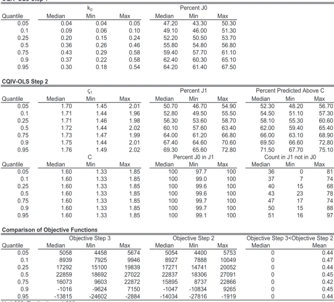
Remark 4

(Step 2). To choose the cut-off

ς

, it is advisable that a constant fraction of

observations satisfying

X

b

i

β

b

(

u

)

> C

are excluded from

J

for each quantile.

To do so,

set

ς

to be the

q

th quantile of

X

b

β

b

(

u

)

−

C

conditional on

X

b

β

b

(

u

)

> C

, where

q

is a

percentage less than

q

(3% worked well in our simulation). In practice, it is desirable that

J

⊂

J

. If this is not the case, we recommend altering

q

,

q

, or the specification of the

regression models. At each quantile, the empirical value of

ς

, the percentage of observations

from the full sample retained in

J

, the percentage of observations from

J

retained in

J

,

and the number of observations in

J

but not in

J

can be computed as simple robustness

diagnostic tests. The estimator

β

b

(

u

) is consistent but will be inefficient relative to the

estimator obtained in the subsequent step.

Remark 5

(Steps 1 and 2). In the notation of Assumption 4, the selector of Step 1 can be

expressed as 1(

S

b

i

b

γ > ς

), where

S

b

b

γ

=

S

b

b

δ

−

Λ

(1

−

u

) and

ς

= Λ

(1

−

u

+

k

)

−

Λ

(1

−

u

).

The selector of Step 2 can also be expressed as 1(

S

b

i

b

γ > ς

)

,

where

S

b

= (

X

b

, C

)

and

b

γ

= (

β

b

(

u

)

,

−

1)

.

Remark 6

(Steps 2, 3 and 4). Beginning with Step 2, each successive iteration of the

algorithm should yield estimates that come closer to minimizing the Powell objective

func-tion. As a simple robustness diagnostic test, we recommend computing the Powell objective

function using the full sample and the estimated coefficients after each iteration, starting

with Step 2. This diagnostic test is computationally straightforward because computing the

objective function for a given set of values is much simpler than maximizing it. In practice,

this test can be used to determine when to stop the CQIV algorithm for each quantile. If

the Powell objective function increases from Step

s

to Step

s

+ 1 for

s

≥

2, estimates from

Step

s

can be retained as the coefficient estimates.

3.2.

Weighted Bootstrap Algorithm.

We recommend obtaining confidence intervals through

a weighted bootstrap procedure, though analytical formulas can also be used. If the

esti-mation runs quickly on the desired sample, it is straightforward to rerun the entire CQIV

algorithm

B

times weighting all the steps by the bootstrap weights. To speed up the

com-putation, we propose a procedure that uses a one-step CQIV estimator in each bootstrap

repetition.

Algorithm 2

(Weighted bootstrap CQIV)

.

For

b

= 1

, . . . , B

, repeat the following steps:

1.

Draw a set of weights

(

e

, . . . , e

)

i.i.d from a random variable

e

that satisfies

As-sumption 6. For example, we can draw the weights from a standard exponential

distribution.

2.

Reestimate the control variable in the weighted sample,

V

b

ib

=

ϑ

b

(

D

, W

, Z

)

, and

construct

X

b

ib

=

x

(

D

, W

,

V

b

)

.

3.

Estimate the weighted quantile regression:

b

β

(

u

) = arg

min

X

e

ρ

(

Y

−

β

X

b

)

,

where

J

=

{

i

:

β

b

(

u

)

X

b

> C

+

ς

}

,

and

β

b

(

u

)

is a consistent estimator of

β

(

u

)

,

e.g., the 3-stage CQIV estimator

β

b

(

u

)

.

Remark 7

(Step 2). The estimate of the control function

ϑ

b

b

can be obtained by weighted

least squares, weighted quantile regression, or weighted distribution regression.

Remark 8

(Step 3). A computationally less expensive alternative is to set

J

=

J

in all the

repetitions, where

J

is the subset of selected observations in Step 2 of the CQIV algorithm.

We can construct an asymptotic (1

−

α

)-confidence interval for a function of the parameter

vector

g

(

β

(

u

)) as [

b

g

,

b

g

], where

b

g

is the sample

α

-quantile of [

g

(

β

b

(

u

))

, . . . , g

(

β

b

(

u

))].

For example, the 0.025 and 0.975 quantiles of (

β

b

1,k

(

u

)

, . . . ,

β

b

(

u

)) form a 95% asymptotic

confidence interval for the

k

th coefficient

β

(

u

).

3.3.

Monte-Carlo illustration.

The goal of the following numerical example is to

com-pare the performance of CQIV relative to tobit IV and other quantile regression estimators

in finite samples. We generate data according to a normal design that satisfies the tobit

parametric assumptions and a design with heteroskedasticity in the first stage equation for

the endogenous regressor

D

that does not satisfy the tobit parametric assumptions. To

facilitate the comparison, in both designs we consider a location model for the response

vari-able

Y

, where the coefficients