San Jose State University
SJSU ScholarWorks
Master's Projects Master's Theses and Graduate Research
Spring 5-20-2019
Machine Learning versus Deep Learning for
Malware Detection
Parth Jain
San Jose State University
Follow this and additional works at:https://scholarworks.sjsu.edu/etd_projects
Part of theArtificial Intelligence and Robotics Commons, and theInformation Security Commons
This Master's Project is brought to you for free and open access by the Master's Theses and Graduate Research at SJSU ScholarWorks. It has been accepted for inclusion in Master's Projects by an authorized administrator of SJSU ScholarWorks. For more information, please contact Recommended Citation
Jain, Parth, "Machine Learning versus Deep Learning for Malware Detection" (2019).Master's Projects. 704. DOI: https://doi.org/10.31979/etd.56y7-b74e
Machine Learning versus Deep Learning for Malware Detection
A Project Presented to
The Faculty of the Department of Computer Science San José State University
In Partial Fulfillment
of the Requirements for the Degree Master of Science
by Parth Jain
© 2019 Parth Jain
The Designated Project Committee Approves the Project Titled Machine Learning versus Deep Learning for Malware Detection
by Parth Jain
APPROVED FOR THE DEPARTMENT OF COMPUTER SCIENCE SAN JOSÉ STATE UNIVERSITY
May 2019
Dr. Mark Stamp Department of Computer Science
Dr. Thomas Austin Department of Computer Science
ABSTRACT
Machine Learning versus Deep Learning for Malware Detection by Parth Jain
It is often claimed that the primary advantage of deep learning is that such models can continue to learn as more data is available, provided that sufficient computing power is available for training. In contrast, for other forms of machine learning it is claimed that models ‘‘saturate,’’ in the sense that no additional learning can occur beyond some point, regardless of the amount of data or computing power available. In this research, we compare the accuracy of deep learning to other forms of machine learning for malware detection, as a function of the training dataset size. We experiment with a wide variety of hyperparameters for our deep learning models, and we compare these models to results obtained using𝑘-nearest neighbors. In these
experiments, we use a subset of a large and diverse malware dataset that was collected as part of a recent research project.
ACKNOWLEDGMENTS
I want to thank Dr. Mark Stamp for selecting me as one of his masters student and having trust in me that I would be able to do this project, for his humorous advice, for teaching the course "Machine Learning with applications in information security", that course really helped me. Another person whom I would like to thank is Professor Fabio Di Troia. For this entire project he was my immediate point of contact, he helped me with each aspect of my project, right from dataset preprocessing to building the final neural network. During this time, I got a chance to know him, and I can certainly say he is cool. I would also like to thank Dr. Thomas Austin for being on my committee and having faith in me that I would be able to complete this project. I would like to thank by brother Nishant Shah for guiding me through out various hurdles of this project. I would also like to thank Dr. Natalia Khuri, because of whom I got so much interest in artificial intelligence and machine learning.
At last I would like to thank my parents, my friends, my family members and all my professors for trusting and supporting me.
TABLE OF CONTENTS
CHAPTER
1 Introduction . . . 1
2 Background . . . 3
2.1 Malware . . . 3
2.2 Machine learning and deep learning . . . 3
2.3 SVM for malware classification . . . 5
2.4 HMM for malware classification . . . 6
2.5 k-NN for malware classification . . . 6
2.6 Deep neural network for malware classification . . . 7
3 Experiments and Results . . . 9
3.1 Dataset . . . 9
3.2 Data preprocessing . . . 10
3.3 Partitioning of the dataset . . . 12
3.4 k-NN experimentation . . . 12
3.5 Neural network experimentation . . . 13
3.6 Results and analysis . . . 14
3.6.1 Malicia dataset . . . 14
3.6.2 Bigdata1 dataset . . . 15
4 Conclusion And Future Work . . . 21
LIST OF REFERENCES . . . 22 APPENDIX
A Result For Malicia Dataset . . . 24 B Result for bigdata1 dataset . . . 28
LIST OF TABLES
1 Malicia dataset details . . . 10
2 Bigdata1 dataset details . . . 11
3 Average accuracy versus size of dataset for𝑘-NN for malicia dataset 14
4 Average accuracy versus size of dataset for neural networks for
Malicia dataset . . . 15
5 Average accuracy versus size of dataset for𝑘-NN for bigdata1
dataset, k:1, test size:10% . . . 16
6 Average accuracy versus size of dataset for deep neural network for
LIST OF FIGURES
1 Average accuracy versus size of dataset for𝑘-NN for Malicia dataset 15
2 Average accuracy versus size of dataset for neural network for
malicia dataset . . . 16
3 Average accuracy versus size of dataset of 𝑘-NN and neural
network for Malicia dataset . . . 17
4 Average accuracy versus size of dataset of 𝑘-NN for bigdata1
dataset, k:1, test size:10% . . . 18
5 Average accuracy versus size of dataset of neural network for
bigdata1 dataset, epochs:200, test size:10% . . . 19
6 Average accuracy versus size of dataset of 𝑘-NN and neural
network for bigdata1 dataset, epochs:200, test size:10%,
activation:softmax, k:1 . . . 20
A.7 Average accuracy vs size of dataset for𝑘-NN and neural network
for Malicia dataset, testsize:0.1, epochs:5,10 . . . 24
A.8 Average accuracy vs size of dataset for𝑘-NN and neural network
for Malicia dataset, testsize:0.1, epochs:50,100 . . . 24
A.9 Average accuracy vs size of dataset for𝑘-NN and neural network
for Malicia dataset, testsize:0.1, epochs:200,1000 . . . 25
A.10 Average accuracy vs size of dataset for𝑘-NN and neural network
for Malicia dataset, testsize:0.2, epochs:5,10 . . . 25
A.11 Average accuracy vs size of dataset for𝑘-NN and neural network
for Malicia dataset, testsize:0.2, epochs:50,100 . . . 25
A.12 Average accuracy vs size of dataset for𝑘-NN and neural network
for Malicia dataset, testsize:0.2, epochs:200,1000 . . . 26
A.13 Average accuracy vs size of dataset for𝑘-NN and neural network
A.14 Average accuracy vs size of dataset for𝑘-NN and neural network
for Malicia dataset, testsize:0.3, epochs:50,100 . . . 26
A.15 Average accuracy vs size of dataset for𝑘-NN and neural network
for Malicia dataset, testsize:0.3, epochs:200,1000 . . . 27
B.16 Average accuracy vs size of dataset for𝑘-NN and neural network
for bigdata1 dataset, testsize:0.1, epochs:5,10 . . . 28
B.17 Average accuracy vs size of dataset for𝑘-NN and neural network
for bigdata1 dataset, testsize:0.1, epochs:50,100 . . . 28
B.18 Average accuracy vs size of dataset for𝑘-NN and neural network
for bigdata1 dataset, testsize:0.1, epochs:200,500 . . . 29
B.19 Average accuracy vs size of dataset for𝑘-NN and neural network
for bigdata1 dataset, testsize:0.2, epochs:5,10 . . . 29
B.20 Average accuracy vs size of dataset for𝑘-NN and neural network
for bigdata1 dataset, testsize:0.2, epochs:50,100 . . . 29
B.21 Average accuracy vs size of dataset for𝑘-NN and neural network
for bigdata1 dataset, testsize:0.2, epochs:200,500 . . . 30
B.22 Average accuracy vs size of dataset for𝑘-NN and neural network
for bigdata1 dataset, testsize:0.3, epochs:5,10 . . . 30
B.23 Average accuracy vs size of dataset for𝑘-NN and neural network
for bigdata1 dataset, testsize:0.3, epochs:50,100 . . . 30
B.24 Average accuracy vs size of dataset for𝑘-NN and neural network
for bigdata1 dataset, testsize:0.3, epochs:200,500 . . . 31
B.25 Average accuracy versus size of dataset of 𝑘-NN and neural
network for bigdata1 dataset, epochs:200, test size:20%,
activation:softmax, k:1 . . . 31
B.26 Average accuracy versus size of dataset of 𝑘-NN and neural
network for bigdata2 dataset, epochs:200, test size:10%,
activation:softmax, k:1 . . . 32
B.27 Average accuracy versus size of dataset of 𝑘-NN and neural
network for bigdata2 dataset, epochs:200, test size:20%,
CHAPTER 1 Introduction
Deep learning and machine learning techniques fall under the domain of artificial intelligence. It is believed that deep learning techniques have tremendous power to solve challenging problems. Both machine learning and deep learning techniques have their advantages and disadvantages based on multiple factors like size of dataset and application. It is very much important to decide which technique is to be used in a particular application.
Deep learning works well when the model is trained for a larger amount of data but for smaller amounts of data the preferred model is machine learning. The graph in [1] purports to show that the accuracy of deep learning models continues to increase, as a function of the training dataset size, after other machine learning techniques have reached a plateau or saturation point. That is, deep learning is generally thought to be superior when the model is trained on large amounts of data. However, for smaller amounts of data, other machine learning techniques may perform better and require significantly less computational effort. In this research, we intend to empirically investigate the trade-off between deep learning and other machine learning techniques, as the size of the training dataset varies over a wide range. We will consider this problem in the context of malware detection, using a recently acquired malware dataset that is larger than any other publicly available dataset [2]. Specifically, in this research, we will compare 𝑘-nearest neighbors (𝑘-NN), to multiple variations of deep
learning techniques. In each case, we will determine the effectiveness of the models as the size of malware training dataset varies over an extremely wide range.
The remainder of this paper is organized as follows. In Chapter 2 we discuss relevant background topics including what is malware, application of machine learning and deep learning on malware dataset, previous popular research work on malware
dataset using machine learning algorithms like Support Vector Machine (SVM),𝑘-NN,
Hidden Markov Model (HMM) and using deep neural networks. In Chapter 3 we discuss about the experimentation details of the project including the dataset used, the preprocessing required, the training phase and the validation phase for 𝑘-NN and
neural networks and we also discuss results and analysis and compare it with [1]. In Chapter 4 we conclude with our findings and also discuss the future works for this project. We also discuss all other results obtained using multiple variation of neural network on the dataset in Appendix A and Appendix B.
CHAPTER 2 Background 2.1 Malware
Before diving more into the details of machine learning and deep learning, it is important to know about the type of data under consideration. For the purpose of this research we will be using a malware dataset [2]. According to [3] malware is a malicious software, designed to damage a computer system without the users informed consent. There are many types of malware, including viruses, worms, trojans, spyware, rootkit.
2.2 Machine learning and deep learning
Machine Learning and deep learning techniques have various kind of application on malware dataset like malware and benign sample classification problem, malware family classification problem. In malware or benign classification problem, given a sample you have to classify whether the sample is malware or benign, whereas for malware family classification problem, the classification is done to classify the malware sample to a specific family of malware.
Machine learning and deep learning techniques can be applied on malware dataset in many ways. One way is to use the operation code (opcode) sequence of the sample. Another such example would be to use binary files. These files can be used in forms like converting them to images or generating 𝑛-grams. We can generate𝑛-grams for
the samples from the binary files or opcode sequence and count the frequency of the each 𝑛-gram and then use it as a feature vector for training machine learning and
deep learning models.
Machine learning and deep learning have three phases, data preprocessing and feature vector generation, training phase and validation phase. In data preprocessing stage, the data is cleaned and a feature vector is generated for the samples. While
training machine learning and deep learning models, the dataset needs to be divided into two parts, the training part and the validating/testing part. In training phase, the training dataset is used to train the model and adjust the parameters for the model to work accurately. In validation phase the validating data is used to test the accuracy of the final trained model. The validation data is never exposed to the model during the training phase.
To measure how well a machine learning or deep learning model works, there are different form of metrics available like accuracy, loss, confusion matrix, area under curve, precision, recall, mean squared error. These are just various ways to see the effectiveness of a model and each of them has their own importance. For the purpose of this research we will just use accuracy, which is the number of samples correctly classified over total number of samples. The entire process of training and validating model needs to be done multiple times, because you are using a part of data for both the phase, so you want to measure the models accuracy when some other part of it is used for training and validating purpose. To do this process effectively, one can use
𝑛-fold cross validation. According to [4], 𝑛-fold cross validation is where a given data
set is split into a n number of sections/folds where each fold is used as a testing set at some point. Let us take the scenario of5-fold cross validation (𝑛= 5). Here, the data
set is split into 5 folds. In the first iteration, the first fold is used to test the model and the rest are used to train the model. In the second iteration, 2nd fold is used as the testing set while the rest serve as the training set. This process is repeated until each fold of the 5 folds have been used as the testing set. You also need to take care of the fact that dataset might be imbalanced, so the data should be partitioned in a way that the imbalance nature of the dataset is handled. One can use stratified
𝑛-fold [5] it is similar to 𝑛-fold but takes care of the imbalance problem.
the malware-benign classification problem and also the malware family classification problem. Researchers have implemented various machine learning algorithms like SVM,𝑘-NN, HMM, Random Forest and also various variants of deep neural networks.
2.3 SVM for malware classification
One popular work [6] uses SVM for malware-benign classification problem. SVM is one of the popular machine learning technique. In a dataset, sometimes there is a need to increase the number of features, SVM increases the dimensionality of the model. This helps to properly separate the dataset into respective classes. A linear SVM is used because the size of the dataset is more than 10,000 samples. A non-linear SVM will not work properly if the number of samples is more than 10,000. In [6] the dataset consisted of 52,803 samples, which consisted of 51,243 malicious samples downloaded from VX Heaven website and 1,560 benign samples from various other sources. The dataset consists of 40 classes. Frequency counting, TFIDF [7] together are used for constructing feature vectors for training SVM. In addition to finding frequency, they also took count of bigrams (sequence of two adjacent words) to construct the feature vector. The bigrams for malware classification are computed in a similar manner as discussed in [8]. During experiment, they constructed 297,003 features of vector per sample. The dataset is divided into training and testing set, where the training set consists of 67% of the whole dataset and testing consist of 33%. This experiment was performed 4 times and each time the training set and testing set was randomly selected. The average accuracy received in [6], for training linear SVM was approximately 75% and the overall accuracy ranges between 74% and 83%, where the number of samples per class is at least 10,000. There is a scope for an improvement in accuracy by studying the features and removing the low weighted features.
2.4 HMM for malware classification
HMM is one of the widely used machine learning algorithms for malware clas-sification problems. In HMM, using the observation sequence and state transition probability, the model tries to predict the label for the sample. The model follows a hill climbing approach, so it needs to be executed multiple times with random restarts, so as to get the maximum accuracy. In [9] an HMM is trained on a dataset consisting of system call logs for 964 malware samples belonging to seven different malware families and 50 benign programs. In [9], system calls are selected as a feature for training an hmm. The dataset is then preprocessed in MIST [10] format. The dataset is converted to𝑛-gram of system calls. In [9], the F-measure score obtained is 0.9994
for malware and 0.6812 for benign samples. For a proper classification of the sample, HMM is combined with Naïve Bayes classifier.
2.5 k-NN for malware classification
One of the most basic machine learning algorithm is 𝑘-NN, lot of research is
done in malware detection using this algorithm. Many times 𝑘-NN has been proved
to be better than other machine learning algorithms. The 𝑘-NN is a non-parametric
method used for classification and regression. In both cases, the input consists of the
𝑘 closest training examples in the feature space. The output depends on whether
𝑘-NN is used for classification or regression. In𝑘-NN classification, the output is a
class membership. An object is classified by a plurality vote of its neighbors, with the object being assigned to the class most common among its 𝑘 nearest neighbors (𝑘
is a positive integer, typically small). If 𝑘 = 1, then the object is simply assigned to
the class of that single nearest neighbor. There are multiple ways of calculating the distance for nearest neighbors like Manhattan distance, Euclidean distance. One of the popular work [11] uses 𝑘-NN for malware classification in HTTPS traffic using
the metric space approach. They have implemented approximate 𝑘-NN search using
metric index and compared it with exponential Chebyshev Minimizer linear classifier. The dataset contains logs of HTTPS connections observed during the period of one day (24 hours) in November 2014 from 500 major international companies collected using Cisco’s cloud web security solution. The dataset consisted of malware and benign samples, all other details can be found in [11].
2.6 Deep neural network for malware classification
Deep learning models are now extensively used for malware classification prob-lems. Deep learning models are originated from neural networks, which are basically originated from perceptron. Perceptron is originated from the artificial neuron. The deep neural network is a combination of multiple such perceptrons with many layers called as a hidden layer, it also has an output layer. The depth of neural network is number of hidden layers, and the width is number of neurons/perceptron per layer. While training a deep neural network, activation function is used like Relu, sigmoid, softmax, Exponential Linear Unit (ELU). The two popular work [12, 13] describes about the usage of deep neural networks for malware classification problem.
In [13] the dataset used is malicia dataset, consisting of 11,308 malware samples and 2,819 benign samples from different windows system. The problem of imbalance of dataset is removed by using the adaptive synthetic technique. The opcode sequence is used as a feature vector for training a deep neural network and the random forest algorithm. In [13], a deep neural network is trained with 2, 4 and 7 layers. All the layers used ELU as the activation function. The results obtained in this paper stated that the random forest algorithm has more accuracy than a deep learning algorithm. The best accuracy obtained by a random forest algorithm was 99.78% whereas by a 7 layer deep neural network was 99.21%.
None of the previous malware analysis work that we are aware of compares deep learning to other machine learning algorithms as the size of the training dataset varies significantly. So, we will be focusing on implementing𝑘-NN and a deep neural network
over different size of datasets and see the nature of the accuracy over the size of dataset.
CHAPTER 3 Experiments and Results
We experimented with𝑘-NN machine learning algorithm and deep neural networks
on malware dataset for malware family classification of the top families of the dataset. Given a sample the algorithm should classify it into either the top families (families having samples more than 1000) or other (sample not belonging to any of the top families) for malicia dataset and for bigdata1 dataset, it should classify it into a malware family.
3.1 Dataset
The datasets used in this research are subset of a much larger dataset [2] which is of around 1 terabyte. We used two dataset, one of them was a smaller dataset called malicia dataset [14] and other one was comparatively larger dataset [15], for the purpose of this research we will call this dataset as bigdata1. malicia dataset [14] was of size 1.5 GB consisting of approximately 11,308 binary files. Details about the malicia dataset are described in Table 1. This dataset has three major families, winwebsec with 4361 files, zbot with 2136 files and zeroaccess with 1305 files. Other families have less than 1000 files. So, to handle such kind of imbalance, we just took 1305 samples from each of the major families because that was the lowest number of samples present in the top major families. From other families, a total of 483 samples were selected, because rest of them were not in proper format. So, the final smaller dataset has 4398 samples. This dataset has 4 labels, 3 of them were the top family names and 4th was for other smaller families.
The bigdata1 dataset [15] was approximately 100 GB but some part of the dataset was excluded as they were not in proper format. This dataset has two major parts comprising of benign samples and malware samples, but for the purpose of this research we just used malware samples, to build malware family classifier. Details
Table 1: Malicia dataset details
Family Samples Present Samples Used
winwebsec 4361 1305
zbot 2136 1305
zeroaccess 1305 1305
other 3506 483
Total 11308 4398
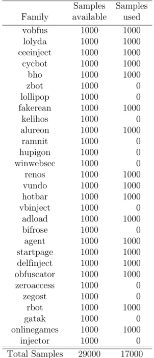
about bigdata1 dataset is described in Table 2. The malware folder consists of 29 folders/families. For this project we just used 1000 files per family but the larger dataset [2] consist of more samples per family. Four folders namely gatak, ramnit, lollipop, and kelihos are from the Microsoft Challenge dataset which were ignored as the bigrams were generated using .bytes files and these families conisit of samples which were hexadecimal representation of bytes. Out of the remaining 25, 5 families vbinject, injector, bifrose, hupigon, and zegost were low-accuracy families which were also ignored. We also ignored the three top families from malicia datset, which were present in this dataset as well. So, the final modified dataset which was used consisted of 17,017 samples with 17 families. The number of labels for this dataset is 17, as there are just 17 classes, and no sample belonging to other families, as we have excluded them. All the samples also consist of a file named top, which has the top 1500 bigram for that family.
3.2 Data preprocessing
For the malicia dataset, we used byte code sequence from the binary files to construct the feature vector. For each sample, we generated bigrams and calculated the frequency of each bigram and stored it into a file named by the sample filename. After getting the bigram frequency for each sample for a family, we clubbed all the bigrams from all the samples belonging to that family and extracted the top 1,000 bigrams for that family. Once top 1,000 bigrams were computed for all the families,
Table 2: Bigdata1 dataset details Samples Samples
Family available used
vobfus 1000 1000 lolyda 1000 1000 ceeinject 1000 1000 cycbot 1000 1000 bho 1000 1000 zbot 1000 0 lollipop 1000 0 fakerean 1000 1000 kelihos 1000 0 alureon 1000 1000 ramnit 1000 0 hupigon 1000 0 winwebsec 1000 0 renos 1000 1000 vundo 1000 1000 hotbar 1000 1000 vbinject 1000 0 adload 1000 1000 bifrose 1000 0 agent 1000 1000 startpage 1000 1000 delfinject 1000 1000 obfuscator 1000 1000 zeroaccess 1000 0 zegost 1000 0 rbot 1000 1000 gatak 1000 0 onlinegames 1000 1000 injector 1000 0 Total Samples 29000 17000
we computed top 1,000 bigrams for the entire dataset using the top 1,000 bigrams for each family. This top 1,000 bigram were used as the feature vector representation for the dataset. Now for each sample we computed the frequency of the top 1,000 bigrams for the dataset and constructed a feature vector for the sample and stored it
in a file along with the label, which was the family name it belonged to.
For the bigdat1 dataset, since we already had the bigrams, for each sample of a family and also the top 1,500 bigrams for each family, so we computed top 1,000 bigrams for the entire dataset using the top 1,500 for each family and then used this top 1,000 bigrams of the entire dataset to compute the feature vector of all the samples in dataset and stored it in a file, similar to the process of malicia dataset.
3.3 Partitioning of the dataset
Since we wanted to run the models for various portions of dataset, so we divided the malicia dataset into 10 portions, i.e 10%, 20%, 30% till 100% of the 4,398 samples. So, 10% comprised of 439 samples. The reason of this partitioning was that we want to see the nature of the accuracy of over the size of dataset. So, now each partition of the dataset is considered as individual dataset. Since we are choosing partitions of dataset randomly, so we made such partitions five times. For example, we took 10% of the data randomly once, did the same thing 4 more times, so that we have five 10% portions of the data. The reason to do this was to cover the entire dataset samples for that partition. All the above partitions were constructed in such a way that it consisted of equal number of samples from all the families, so that there is no imbalance of data in the partitions. Similarly, the portions were made for the bigdata1 dataset. 10% portion of bigdata1 consisted of 1,700 samples.
3.4 k-NN experimentation
We experimented with 𝑘-NN algorithm for all 𝑘 value ranging from 1 to 10. For
each 𝑘 value we did a 𝑛-fold cross validation with 10 folds. So, for each partition we
ran the algorithm 5 time for all 𝑘 values and during every iteration of 𝑘 value we did
a 10 fold cross validation and then average value of the accuracy is computed for all the 𝑘 values and then for all the 5 partitions. i.e if we consider 10% of data then we
have 5 sets with 10% of the data. So, we ran the algorithm 5 times and during each iteration, we have 10 𝑘 values, so we trained the model for all the 𝑘 values and then
during each iteration of 𝑘 value we did a 10 fold cross validation. So, in all we trained
500𝑘-NN models, for each of the 5 iterations, during every iteration we trained the
model for 10 𝑘 values and for each of the 10 partitions.
5 (sets of partition)×10 (𝑘 values)×10 (total number of partition) = 500
We got average value of accuracy for each partition. We used stratified 𝑘-fold and 𝑘-NN from sklearn library [5]. Stratified𝑘-fold takes care of taking data in a balanced
form, i.e. taking equal data from all the families.
3.5 Neural network experimentation
Similar to 𝑘-NN, we experimented with neural networks. The neural network
consisted of one input layer, two hidden layer and one output layer. The input layer consists of 1000 input nodes. The two hidden layer consists of 128 nodes each with relu as the activation function. Output layer comprises of 4 nodes for the malicia dataset with softmax as the activation function, because the class label for the sample can be either the three major family in the malicia dataset or other, so 4 labels. For the bigdata1 dataset, the number of class labels are 17, so the output layer consists of 17 nodes with softmax as the activation function. For neural networks also the data was partitioned into various percentages and then used. We ran the algorithm for 5, 10, 50, 100, 200, 500, and 1000 epochs, and also for various test sizes like 10%, 20%, 30%. Similar to𝑘-NN we ran the model for 5 iterations for each value of epoch and
test size and then averaged the accuracy for that partition for the value of epoch and test size. So, for each value of epoch and test size, the number of models trained are 50 times number of epochs, for each of the 5 iteration, and for each of the 10 partition, model was trained for total number of epochs. Thus, each experiment consists of
training50×𝐸 models, where𝐸 is the the number of epochs. We also experimented
with sigmoid as the activation function in output layer, though sigmoid is generally used for binary class classification, it performed similar to softmax.
3.6 Results and analysis
In this section we will be discussing about the results obtained based on the above experimentation for malicia dataset and bigdata1 dataset. We will also be analyzing the results and comparing it with claims made by [1].
3.6.1 Malicia dataset
The average value of accuracy obtained for each partition by running 𝑘-NN
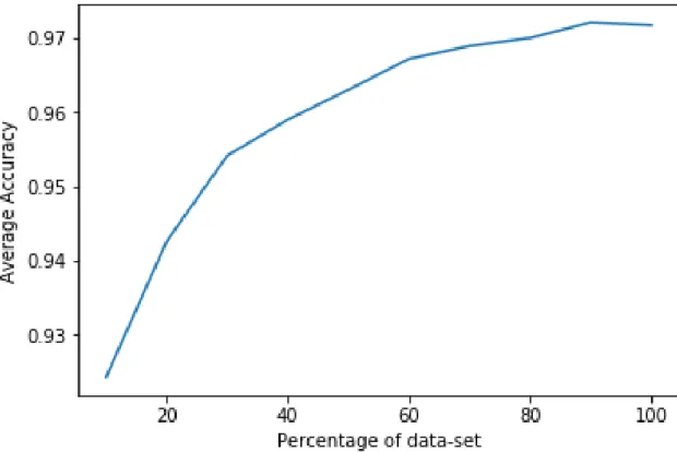
algorithm can be found in Table 3. Figure 1 represents the average accuracy as the size of the dataset increases for 𝑘-NN for malicia dataset. The graph for 𝑘-nn is
smooth and increases as the size of dataset is increasing. The max accuracy received is 97.21%. Though there is a slight drop from 90% dataset to 100% dataset, this drop is of 0.03%. So, we can neglect this change. So, we can say that the graph remains constant between 90% and 100% of dataset. The accuracy received was highest with test size is 10% and 𝑘 is 1.
Table 3: Average accuracy versus size of dataset for 𝑘-NN for malicia dataset
10% 20% 30% 40% 50% 60% 70% 80% 90% 100%
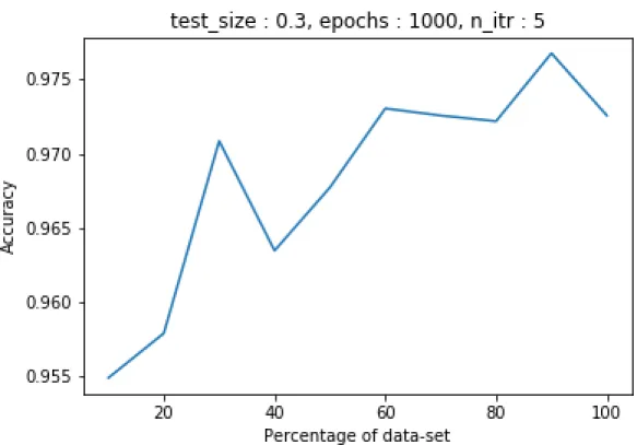
0.9243 0.9426 0.9541 0.9590 0.9630 0.9672 0.9689 0.9700 0.9721 0.9718 The results obtained by running deep neural network for multiple values of epochs and test sizes were interesting. The maximum accuracy was received for 1,000 epochs and 30% test size for 90% partition. The value of accuracy over different partitions are described in Table 4. The overall graph increases from 10% dataset to 100% dataset. But in between the accuracy value is increasing and decreasing, but overall it increases. Figure 2 supports this analysis.
Figure 1: Average accuracy versus size of dataset for𝑘-NN for Malicia dataset
Table 4: Average accuracy versus size of dataset for neural networks for Malicia dataset
10% 20% 30% 40% 50% 60% 70% 80% 90% 100%
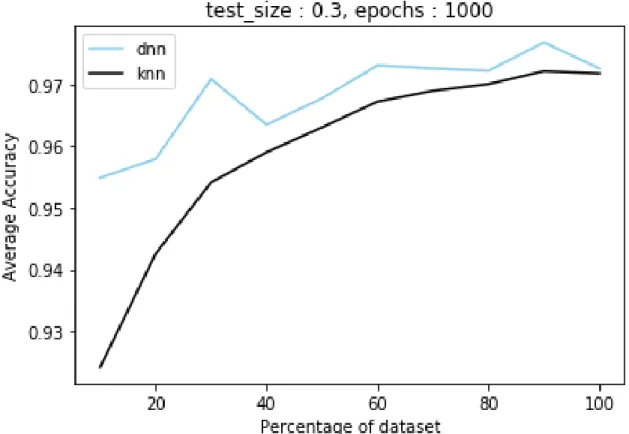
0.9549 0.9579 0.9709 0.9635 0.9677 0.9730 0.9726 0.9722 0.9768 0.9726 From Figure 3 it can be concluded that for a malicia dataset neural networks performed better than 𝑘-NN algorithm. The graph in Figure 3 is not similar to the
one in [1].
3.6.2 Bigdata1 dataset
The results obtained for 𝑘-NN for bigdata1 dataset follows the similar pattern,
with the value of accuracy increasing as the size of dataset increases, except that the
accuracy for 𝑘-NN does not seem to be saturating between 90% and 100% dataset,
Figure 2: Average accuracy versus size of dataset for neural network for malicia dataset
for 𝑘-NN over different size of dataset with test size 10% and 𝑘 value as 1. We also
experimented with test size 20% but the best accuracy was for 10% with 𝑘 value as 1.
The average value of accuracy obtained for each partition by running𝑘-NN algorithm
for 10% test size and 𝑘 = 1 are in Table 5. Maximum value of accuracy received
was 87.07% for 100% partition, though it is less as compared to the 𝑘-NN result for
malicia dataset, but these two results can not be compared with each other due to dataset difference and number of major family difference.
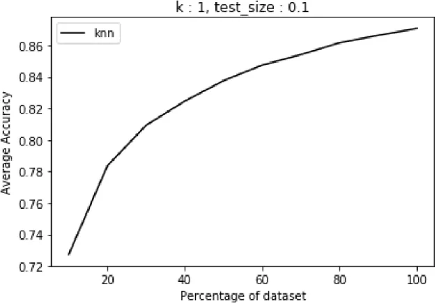
Table 5: Average accuracy versus size of dataset for 𝑘-NN for bigdata1 dataset, k:1,
test size:10%
10% 20% 30% 40% 50% 60% 70% 80% 90% 100%
Figure 3: Average accuracy versus size of dataset of 𝑘-NN and neural network for
Malicia dataset
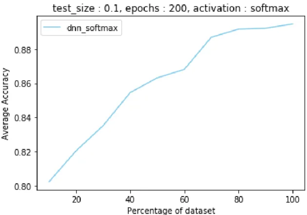
In case of neural network, the best case accuracy was obtained for epochs 200 with test size 10%. We also experimented with 20% as test size. The best case accuracy value over size of dataset for our neural network experiments using the bigdata1 dataset are given in Table 6. The accuracy versus size of dataset graph in Figure 5 for this case is not similar to Figure 2. The graph is continuously increasing with increase in size of dataset and the graph has a smooth increasing curve. The maximum accuracy is 89.47% for 200 epochs with 10% as the test data size which is
more than the maximum accuracy for 𝑘-NN.
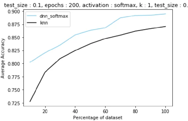
The result From Figure 6 we can see that deep learning accuracy is always greater
Figure 4: Average accuracy versus size of dataset of 𝑘-NN for bigdata1 dataset, k:1,
test size:10%
Table 6: Average accuracy versus size of dataset for deep neural network for bigdata1 dataset, epochs:200, test size:10%
10% 20% 30% 40% 50% 60% 70% 80% 90% 100%
[0.8023 0.8205 0.8352 0.8545 0.8631 0.8681 0.8869 0.8916 0.8922 0.8947 accuracy value for both the algorithms decreases as the size of dataset increases and also the accuracy for both the graph increases with increases in dataset.
From both Figure 3 and Figure 6, we can say that deep learning accuracy is always greater than machine learning accuracy. So, the claim by [1], that machine learning accuracy is more than deep learning accuracy for smaller dataset and for larger dataset deep learning has more accuracy does not holds true. We also did not get any intersections point where deep learning accuracy and machine learning
Figure 5: Average accuracy versus size of dataset of neural network for bigdata1 dataset, epochs:200, test size:10%
accuracy is same. One of the interesting thing which can be seen in Figure 6 is that both algorithms perform better as the size of dataset increases, and we can see the values getting closer with increase in dataset size. Looking at the nature of both the curves in Figure 6 they both will tend to increase with increase in dataset. Also, the claim that machine learning accuracy will saturate after a point, also does not holds true, in spite of the fact that in malicia dataset the accuracy was constant between 90% data and 100% data, but we did not see a similar trend in bigdata1 dataset. We can also see that machine learning and deep learning accuracy are over all increasing over size of dataset. Furthermore, it seems that, if we add more data, the accuracy will increase in both the cases. Though one of the claims by [1] partially holds true,
that deep learning accuracy keeps increasing with the increase in size of dataset, but for mailica dataset the neural network curve has few sudden decrease in the value of accuracy but over value of accuracy has increased.
Figure 6: Average accuracy versus size of dataset of 𝑘-NN and neural network for
CHAPTER 4
Conclusion And Future Work
Machine learning and deep learning both have there own pros and cons. In this paper we experimented with 𝑘-NN and neural networks on malicia dataset and
bigdata1 dataset and generated average value of accuracy over size of dataset. We compared these graphs with the graph in [1]. We saw that the graphs generated based on our experiments does not match with the one in [1]. From our experiments deep learning accuracy was always greater than machine learning accuracy even for the smallest partition of the dataset. We did not find any intersection point for 𝑘-NN
and neural networks as show in [1]. We were also able to see that machine learning and deep learning has an increase in accuracy as the size of dataset increases and the difference between the accuracy for𝑘-NN and neural network decreases with increases
in size of dataset.
This research paper was just focused on two sub datasets from the much larger dataset of 1 terabyte. There is a lot of future work involved to claim about the actual nature of graph of machine learning and deep learning over size of dataset. We need to experiment with these algorithms over the entire larger dataset and with more variations in hyper parameter. We also need to experiment with other machine learning and deep learning algorithms over the larger dataset. Since we never found a point where machine learning accuracy was more than deep learning then one of the future works would be to find the value of the smallest dataset size, where machine learning accuracy will be more than deep learning. There is another future work involved to experiment with different types of features and not just bigrams, like other𝑛-grams, opcode sequence, converting the byte files to images. Trying on other
form of problems like malware-benign sample classification problem would be also an interesting future work.
LIST OF REFERENCES
[1] Kaggle, ‘‘Deep learning vs machine learning efficiency over size of data,’’ https: //ibb.co/m2bxcc, Mar 2018, (Accessed on 10/01/2018).
[2] S. Kim, ‘‘PE header analysis for malware detection,’’ Master’s Project, Depart-ment of Computer Science, San Jose State University, 2018, https://scholarworks. sjsu.edu/etd_projects/624/.
[3] N. Bhojani, ‘‘Malware analysis,’’ in Ethical Hacking Conference, At Nirma
University, 10 2014.
[4] K. Hewa, ‘‘K-fold cross validation,’’ https://medium.com/datadriveninvestor/k-fold-cross-validation-6b8518070833, Dec 2018, (Accessed on 10/01/2018). [5] F. Pedregosa, G. Varoquaux, A. Gramfort, V. Michel, B. Thirion, O. Grisel,
M. Blondel, P. Prettenhofer, R. Weiss, V. Dubourg, J. Vanderplas, A. Passos, D. Cournapeau, M. Brucher, M. Perrot, and E. Duchesnay, ‘‘Scikit-learn: Machine learning in Python,’’ Journal of Machine Learning Research, vol. 12, pp.
2825--2830, 2011.
[6] B. Sanjaa and E. Chuluun, ‘‘Malware detection using linear svm,’’ in Ifost, vol. 2,
June 2013, pp. 136--138.
[7] P. Soucy and G. W. Mineau, ‘‘A simple knn algorithm for text categorization,’’ inProceedings 2001 IEEE International Conference on Data Mining, Nov 2001,
pp. 647--648.
[8] E. Raff, R. Zak, R. J. Cox, J. Sylvester, P. Yacci, R. Ward, A. Tracy, M. McLean, and C. Nicholas, ‘‘An investigation of byte n-gram features for malware classi-fication,’’ Journal of Computer Virology and Hacking Techniques, vol. 14, pp.
1--20, 2016.
[9] M. Imran, M. T. Afzal, and M. A. Qadir, ‘‘Similarity-based malware classification using hidden markov model,’’ in 2015 Fourth International Conference on Cyber Security, Cyber Warfare, and Digital Forensic (CyberSec), Oct 2015, pp. 129--134.
[10] P. Trinius, C. Willems, T. Holz, and K. Rieck, ‘‘A malware instruction set for behavior-based analysis.’’ in Sicherheit 2010: Sicherheit, Schutz und Zuverläs-sigkeit, Beiträge der 5. Jahrestagung des Fachbereichs Sicherheit der Gesellschaft für Informatik e.V. (GI), 5.-7. Oktober 2010 in Berlin., 01 2010, pp. 205--216.
[11] J. Lokoč, J. Kohout, P. Čech, T. Skopal, and T. Pevný, ‘‘k-nn classification of malware in https traffic using the metric space approach,’’ in Intelligence and Security Informatics, M. Chau, G. A. Wang, and H. Chen, Eds. Cham: Springer
International Publishing, 2016, pp. 131--145.
[12] B. Cakir and E. Dogdu, ‘‘Malware classification using deep learning
methods,’’ in Proceedings of the ACMSE 2018 Conference, ser. ACMSE
’18. New York, NY, USA: ACM, 2018, pp. 10:1--10:5. [Online]. Available: http://doi.acm.org/10.1145/3190645.3190692
[13] M. Sewak, S. K. Sahay, and H. Rathore, ‘‘Comparison of deep learning and
the classical machine learning algorithm for the malware detection,’’ 2018
19th IEEE/ACIS International Conference on Software Engineering, Artificial Intelligence, Networking and Parallel/Distributed Computing (SNPD), Jun 2018.
[Online]. Available: http://dx.doi.org/10.1109/SNPD.2018.8441123
[14] ‘‘Malicia malware dataset,’’ https://mega.nz/#!LdFHyIqJ!
H9zOeQL3z6m24t2Bz0PaQqlR026b74Ws3Uys4Kooc9c, (Accessed on
10/01/2018).
[15] Sam, ‘‘Bigrams for 100gb dataset,’’ https://github.com/bsamanvitha/298_ Dataset, (Accessed on 03/01/2019).
APPENDIX A Result For Malicia Dataset
The graphs below are from various tests performed on Malicia dataset using𝑘-NN
algorithm and neural network algorithm.
(a) testsize:0.1, epochs:5 (b) testsize:0.1, epochs:10
Figure A.7: Average accuracy vs size of dataset for 𝑘-NN and neural network for
Malicia dataset, testsize:0.1, epochs:5,10
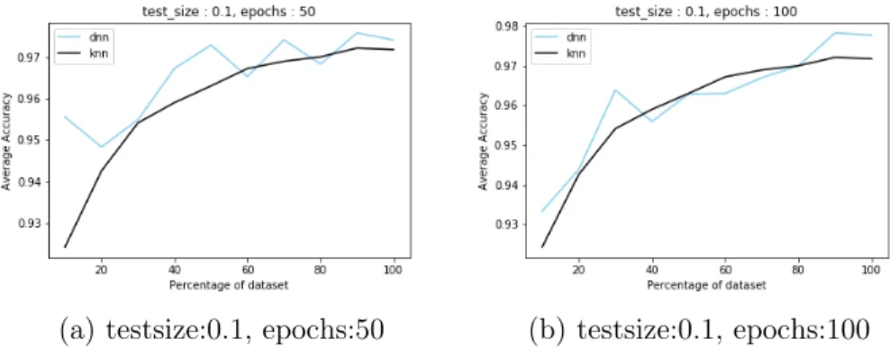
(a) testsize:0.1, epochs:50 (b) testsize:0.1, epochs:100
Figure A.8: Average accuracy vs size of dataset for 𝑘-NN and neural network for
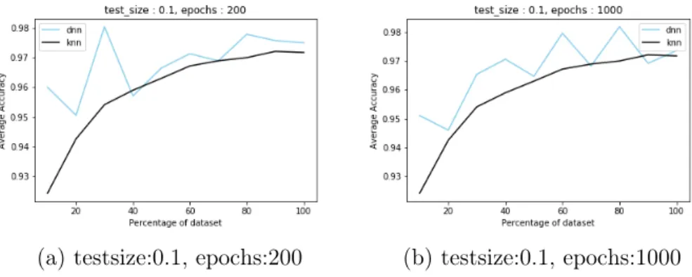
(a) testsize:0.1, epochs:200 (b) testsize:0.1, epochs:1000
Figure A.9: Average accuracy vs size of dataset for 𝑘-NN and neural network for
Malicia dataset, testsize:0.1, epochs:200,1000
(a) testsize:0.2, epochs:5 (b) testsize:0.2, epochs:10
Figure A.10: Average accuracy vs size of dataset for 𝑘-NN and neural network for
Malicia dataset, testsize:0.2, epochs:5,10
(a) testsize:0.2, epochs:50 (b) testsize:0.2, epochs:100
Figure A.11: Average accuracy vs size of dataset for 𝑘-NN and neural network for
(a) testsize:0.2, epochs:200 (b) testsize:0.2, epochs:1000
Figure A.12: Average accuracy vs size of dataset for 𝑘-NN and neural network for
Malicia dataset, testsize:0.2, epochs:200,1000
(a) testsize:0.3, epochs:5 (b) testsize:0.3, epochs:10
Figure A.13: Average accuracy vs size of dataset for 𝑘-NN and neural network for
Malicia dataset, testsize:0.3, epochs:5,10
(a) testsize:0.3, epochs:50 (b) testsize:0.3, epochs:100
Figure A.14: Average accuracy vs size of dataset for 𝑘-NN and neural network for
(a) testsize:0.3, epochs:200 (b) testsize:0.3, epochs:1000
Figure A.15: Average accuracy vs size of dataset for 𝑘-NN and neural network for
APPENDIX B
Result for bigdata1 dataset
The graphs below are from various tests performed on bigdata1 dataset using
𝑘-NN algorithm and neural network algorithm. Neural network has sigmoid as the
activation function for output layer.
(a) testsize:0.1, epochs:5 (b) testsize:0.1, epochs:10
Figure B.16: Average accuracy vs size of dataset for 𝑘-NN and neural network for
bigdata1 dataset, testsize:0.1, epochs:5,10
(a) testsize:0.1, epochs:50 (b) testsize:0.1, epochs:100
Figure B.17: Average accuracy vs size of dataset for 𝑘-NN and neural network for
bigdata1 dataset, testsize:0.1, epochs:50,100
We also experimented with bigdata2, which was also a subset of the same bigger dataset. Bigdata2 consisted of a total of 36575 samples, from 19 different families. These 19 families are from the same 29 families from bigdata1. For bigdata1 experimentation we just used 17 families. Bigdata2, consisted of 1925 samples from
(a) testsize:0.1, epochs:200 (b) testsize:0.1, epochs:500
Figure B.18: Average accuracy vs size of dataset for 𝑘-NN and neural network for
bigdata1 dataset, testsize:0.1, epochs:200,500
(a) testsize:0.2, epochs:5 (b) testsize:0.2, epochs:10
Figure B.19: Average accuracy vs size of dataset for 𝑘-NN and neural network for
bigdata1 dataset, testsize:0.2, epochs:5,10
(a) testsize:0.2, epochs:50 (b) testsize:0.2, epochs:100
Figure B.20: Average accuracy vs size of dataset for 𝑘-NN and neural network for
bigdata1 dataset, testsize:0.2, epochs:50,100
each of the 19 families. Figure B.26 and Figure B.27 shows the results obtained by running 𝑘-nn and neural networks on bigdata2.
(a) testsize:0.2, epochs:200 (b) testsize:0.2, epochs:500
Figure B.21: Average accuracy vs size of dataset for 𝑘-NN and neural network for
bigdata1 dataset, testsize:0.2, epochs:200,500
(a) testsize:0.3, epochs:5 (b) testsize:0.3, epochs:10
Figure B.22: Average accuracy vs size of dataset for 𝑘-NN and neural network for
bigdata1 dataset, testsize:0.3, epochs:5,10
(a) testsize:0.3, epochs:50 (b) testsize:0.3, epochs:100
Figure B.23: Average accuracy vs size of dataset for 𝑘-NN and neural network for
(a) testsize:0.3, epochs:200 (b) testsize:0.3, epochs:500
Figure B.24: Average accuracy vs size of dataset for 𝑘-NN and neural network for
bigdata1 dataset, testsize:0.3, epochs:200,500
Figure B.25: Average accuracy versus size of dataset of 𝑘-NN and neural network for
Figure B.26: Average accuracy versus size of dataset of 𝑘-NN and neural network for
Figure B.27: Average accuracy versus size of dataset of 𝑘-NN and neural network for