When Worlds Collide: Integrating Different
Counterfactual Assumptions in Fairness
Chris Russell∗ The Alan Turing Institute and
University of Surrey crussell@turing.ac.uk
Matt J. Kusner∗ The Alan Turing Institute and
University of Warwick mkusner@turing.ac.uk
Joshua R. Loftus† New York University
loftus@nyu.edu
Ricardo Silva The Alan Turing Institute and
University College London ricardo@stats.ucl.ac.uk
Abstract
Machine learning is now being used to make crucial decisions about people’s lives. For nearly all of these decisions there is a risk that individuals of a certain race, gender, sexual orientation, or any other subpopulation are unfairly discriminated against. Our recent method has demonstrated how to use techniques from coun-terfactual inference to make predictions fair across different subpopulations. This method requires that one provides the causal model that generated the data at hand. In general, validating all causal implications of the model is not possible without further assumptions. Hence, it is desirable to integrate competing causal models to provide counterfactually fair decisions, regardless of which causal “world” is the correct one. In this paper, we show how it is possible to make predictions that are approximately fair with respect to multiple possible causal models at once, thus mitigating the problem of exact causal specification. We frame the goal of learning a fair classifier as an optimization problem with fairness constraints entailed by competing causal explanations. We show how this optimization problem can be efficiently solved using gradient-based methods. We demonstrate the flexibility of our model on two real-world fair classification problems. We show that our model can seamlessly balance fairness in multiple worlds with prediction accuracy.
1
Introduction
Machine learning algorithms can do extraordinary things with data. From generating realistic images from noise [7], to predicting what you will look like when you become older [18]. Today, governments and other organizations make use of it in criminal sentencing [4], predicting where to allocate police officers [3, 16], and to estimate an individual’s risk of failing to pay back a loan [8]. However, in many of these settings, the data used to train machine learning algorithms contains biases against certain races, sexes, or other subgroups in the population [3, 6]. Unwittingly, this discrimination is then reflected in the predictions of such algorithms. Simply being born male or female can change an individual’s opportunities that follow from automated decision making trained to reflect historical biases. The implication is that, without taking this into account, classifiers that maximize accuracy risk perpetuating biases present in society.
∗
Equal contribution.
†
This work was done while JL was a Research Fellow at the Alan Turing Institute.
For instance, consider the rise of ‘predictive policing’, described as “taking data from disparate sources, analyzing them, and then using the results to anticipate, prevent and respond more effectively to future crime” [16]. Today,38%of U.S. police departments surveyed by the Police Executive Research Forum are using predictive policing and70%plan to in the next2to5years. However, there have been significant doubts raised by researchers, journalists, and activists that if the data used by these algorithms is collected by departments that have been biased against minority groups, the predictions of these algorithms could reflect that bias [9, 12].
At the same time, fundamental mathematical results make it difficult to design fair classifiers. In criminal sentencing the COMPAS score [4] predicts if a prisoner will commit a crime upon release, and is widely used by judges to set bail and parole. While it has been shown that black and white defendants with the same COMPAS score commit a crime at similar rates after being released [1], it was also shown that black individuals were more often incorrectly predicted to commit crimes after release by COMPAS than white individuals were [2]. In fact, except for very specific cases, it is impossible to balance these measures of fairness [3, 10, 20].
The question becomes how to address the fact that the data itself may bias the learning algorithm and even addressing this is theoretically difficult. One promising avenue is a recent approach, introduced by us in [11], calledcounterfactual fairness. In this work, we model how unfairness enters a dataset using techniques from causal modeling. Given such a model, we state whether an algorithm is fair if it would give the same predictions had an individual’s race, sex, or other sensitive attributes been different. We show how to formalize this notion using counterfactuals, following a rich tradition of causal modeling in the artificial intelligence literature [15], and how it can be placed into a machine learning pipeline. The big challenge in applying this work is that evaluating a counterfactual e.g., “What if I had been born a different sex?”, requires a causal model which describes how your sex
changes your predictions, other things being equal.
Using “world” to describe any causal model evaluated at a particular counterfactual configuration, we have dependent “worlds” within asamecausal model that can never be jointly observed, and possibly incompatible “worlds” acrossdifferentmodels. Questions requiring the joint distribution of counterfactuals are hard to answer, as they demand partially untestable “cross-world” assumptions [5, 17], and even many of the empirically testable assumptions cannot be falsified from observational data alone [14], requiring possibly infeasible randomized trials. Because of this, different experts as well as different algorithms may disagree about the right causal model. Further disputes may arise due to the conflict between accurately modeling unfair data and producing a fair result, or because some degrees of unfairness may be considered allowable while others are not.
To address these problems, we propose a method for ensuring fairness within multiple causal models. We do so by introducing continuous relaxations of counterfactual fairness. With these relaxations in hand, we frame learning a fair classifier asan optimization problem with fairness constraints. We give efficient algorithms for solving these optimization problems for different classes of causal models. We demonstrate on three real-world fair classification datasets how our model is able to simultaneously achieve fairness in multiple models while flexibly trading off classification accuracy.
2
Background
We begin by describing aspects causal modeling and counterfactual inference relevant for modeling fairness in data. We then briefly review counterfactual fairness [11], but we recommend that the interested reader should read the original paper in full. We describe how uncertainty may arise over the correct causal model and some difficulties with the original counterfactual fairness definition. We will useAto denote the set of protected attributes, a scalar in all of our examples but which without loss of generality can take the form of a set. Likewise, we denote asY the outcome of interest that needs to be predicted using a predictorYˆ. Finally, we will useXto denote the set of observed variables other thanAandY, andU to denote a set of hidden variables, which without loss of generality can be assumed to have no observable causes in a corresponding causal model. 2.1 Causal Modeling and Counterfactual Inference
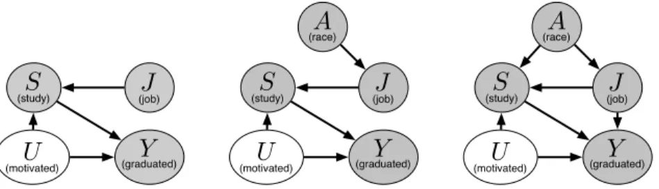
We will use the causal framework of Pearl [15], which we describe using a simple example. Imagine we have a dataset of university students and we would like to model the causal relationships that
(study) (job) (graduated)
J
S
Y
(motivated)U
(race) (study) (job) (graduated)A
J
S
Y
(motivated)U
(race) (study) (job) (graduated)A
J
S
Y
(motivated)U
Figure 1: Dark nodes correspond to observed variables and light nodes are unobserved. (Left) This model predicts that both studySand motivationUdirectly cause graduation rateY. However, this model does not take into account how an individual’s race may affect observed variables. (Center) In this model, we encode how an individual’s race may affect whether they need to have a jobJ while attending university. (Right) We may wonder if there are further biases in society to expect different rates of study for different races. We may also suspect that having a job may influence one’s graduation likelihood, independent of study.
lead up to whether a student graduates on time. In our dataset, we have information about whether a student holds a jobJ, the number of hours they study per weekS, and whether they graduate Y. Because we are interested in modeling any unfairness in our data, we also have information about a student’s raceA. Pearl’s framework allows us to model causal relationships between these variables and any postulated unobserved latent variables, such as someUquantifying how motivated a student is to graduate. This uses a directed acyclic graph (DAG) with causal semantics, called a causal diagram. We show a possible causal diagram for this example in Figure 1, (Left). Each node corresponds to a variable and each set of edges into a node corresponds to a generative model specifying how the “parents” of that node causally generated it. In its most specific description, this generative model is a functional relationship deterministically generating its output given a set of observed and latent variables. For instance, one possible set of functions described by this model could be as follows:
S=g(J, U) + Y =I[φ(h(S, U))≥0.5] (1)
whereg, hare arbitrary functions andIis the indicator function that evaluates to1if the condition
holds and0otherwise. Additionally,φis the logistic functionφ(a) = 1/(1 + exp(−a))andis drawn independently of all variables from the standard normal distributionN(0,1). It is also possible to specify non-deterministic relationships:
U ∼ N(0,1) S∼ N(g(J, U), σS) Y ∼Bernoulli(φ(h(S, U)) (2) where σS is a model parameter. The power of this causal modeling framework is that, given a fully-specified set of equations, we can compute what (the distribution of) any of the variables would have beenhad certain other variables been different, other things being equal. For instance, given the causal model we can ask “Would individualihave graduated (Y= 1) if they hadn’t had a job?”, even if they did not actually graduate in the dataset. Questions of this type are calledcounterfactuals. For any observed variablesV, W we denote the value of the counterfactual “What wouldV have been ifW had been equal tow?” as VW←w. Pearl et al. [15] describe how to compute these counterfactuals (or, for non-deterministic models, how to compute their distribution) using three steps: 1.Abduction: Given the set of observed variablesX={X1, . . . , Xd}compute the values of the set of unobserved variablesU={U1, . . . , Up}given the model (for non-deterministic models, we compute the posterior distributionP(U |X)); 2.Action: Replace all occurrences of the variable W with valuewin the model equations; 3.Prediction: Using the new model equations, andU (or
P(U |X)) compute the value ofV (orP(V|X)). This final step provides the value or distribution of
VW←wgiven the observed, factual, variables. 2.2 Counterfactual Fairness
In the above example, the university may wish to predictY, whether a student will graduate, in order to determine if they should admit them into an honors program. While the university prefers to admit students who will graduate on time, it is willing to give a chance to some students without a confident graduation prediction in order to remedy unfairness associated with race in the honors
program. The university believes that whether a student needs a jobJmay be influenced by their race. As evidence they cite the National Center for Education Statistics, which reported3that fewer (25%) Asian-American students were employed while attending university as full-time students relative to students of other races (at least 35%). We show the corresponding casual diagram for this in Figure 1 (Center). As having a jobJ affects study which affects graduation likelihoodY this may mean different races take longer to graduate and thus unfairly have a harder time getting into the honors program.
Counterfactual fairnessaims to correct predictions of a label variableY that are unfairly altered by an individual’s sensitive attributeA(race in this case). Fairness is defined in terms of counterfactuals: Definition 1(Counterfactual Fairness [11]). A predictorYˆ ofY iscounterfactually fairgiven the sensitive attributeA=aand any observed variablesX if
P( ˆYA←a=y| X =x, A=a) =P( ˆYA←a0=y| X =x, A=a) (3)
for allyanda06=a.
In what follows, we will also refer toYˆ as a functionf(x, a)of hidden variablesU, of (usually a subset of) an instantiationxofX, and of protected attributeA. We leaveU implicit in this notation since, as we will see, this set might differ across different competing models. The notation implies
ˆ
YA←a=f(xA←a, a). (4)
Notice that if counterfactual fairness holds exactly forYˆ, then this predictor can only be a non-trivial function ofX for those elementsX ∈ X such thatXA←a =XA←a0. Moreover, by construction
UA←a=UA←a0, as each element ofU is defined to have no causes inA∪ X.
The probabilities in eq. (3) are given by the posterior distribution over the unobserved variables
P(U | X =x, A=a). Hence, a counterfactualYˆA←a may bedeterministicif this distribution is degenerate, that is, ifU is a deterministic function ofXandA. One nice property of this definition is that it is easy to interpret: a decision is fair if it would have been the same had a person had a differentA(e.g., a different race4), other things being equal. In [11], we give an efficient algorithm for designing a predictor that is counterfactually fair. In the university graduation example, a predictor constructed from the unobserved motivation variableU is counterfactually fair.
One difficulty of the definition of counterfactual fairness is it requires one to postulate causal relationships between variables, including latent variables that may be impractical to measure directly. In general, different causal models will create different fair predictorsYˆ. But there are several reasons why it may be unrealistic to assume that any single, fixed causal model will be appropriate. There may not be a consensus among experts or previous literature about the existence, functional form, direction, or magnitude of a particular causal effect, and it may be impossible to determine these from the available data without untestable assumptions. And given the sensitive, even political nature of problems involving fairness, it is also possible that disputes may arise over the presence of a feature of the causal model, based on competing notions of dependencies and latent variables. Consider the following example, formulated as a dispute over the presence of edges. For the university graduation model, one may ask if differences in study are due only to differences in employment, or whether instead there is some other direct effect ofAon study levels. Also, having a job may directly affect graduation likelihood. We show these changes to the model in Figure 1 (Right). There is also potential for disagreement over whether some causal paths fromAto graduation should be excluded from the definition of fairness. For example, an adherent to strict meritocracy may argue the numbers of hours a student has studied should not be given a counterfactual value. This could be incorporated in a separate model by omitting chosen edges when propagating counterfactual information through the graph in thePredictionstep of counterfactual inference5. To summarize, there may be disagreements about the right causal model due to: 1. Changing the structure of the DAG, e.g. adding an edge; 2. Changing the latent variables, e.g. changing the function generating a vertex to have a different signal vs. noise decomposition; 3. Preventing certain paths from propagating counterfactual values.
3https://nces.ed.gov/programs/coe/indicator_ssa.asp 4
At the same time, the notion of a “counterfactual race,” sex, etc. often raises debate. See [11] for our take on this.
5
In the Supplementary Material of [11], we explain how counterfactual fairness can be restricted to particular paths fromAtoY, as opposed to all paths.
3
Fairness under Causal Uncertainty
In this section, we describe a technique for learning a fair predictor without knowing the true casual model. We first describe why in general counterfactual fairness will often not hold in multiple different models. We then describe a relaxation of the definition of counterfactual fairness for both deterministic and non-deterministic models. Finally we show an efficient method for learning classifiers that are simultaneously accurate and fair in multiple worlds. In all that follows we denote sets in calligraphic scriptX, random variables in uppercaseX, scalars in lowercasex, matrices in bold uppercaseX, and vectors in bold lowercasex.
3.1 Exact Counterfactual Fairness Across Worlds
We can imagine extending the definition of counterfactual fairness so that it holds for every plausible causal world. To see why this is inherently difficult consider the setting of deterministic causal models. If each causal model of the world generates different counterfactuals then each additional model induces a new set of constraints that the classifier must satisfy, and in the limit the only classifiers that are fair across all possible worlds are constant classifiers. For non-deterministic counterfactuals, these issues are magnified. To guarantee counterfactual fairness, Kusner et al. [11] assumed access to latent variables that hold the same value in an original datapoint and in its corresponding counterfactuals. While the latent variables of one world can remain constant under the generation of counterfactuals from its corresponding model, there is no guarantee that they remain constant under the counterfactuals generated from different models. Even in a two model case, if the P.D.F. of one model’s counterfactual has non-zero density everywhere (as is the case under Gaussian noise assumptions) it may be the case that the only classifiers that satisfy counterfactual fairness for both worlds are the constant classifiers. If we are to achieve some measure of fairness from informative classifiers, and over a family of different worlds, we need a more robust alternative to counterfactual fairness.
3.2 Approximate Counterfactual Fairness
We define two approximations to counterfactual fairness to solve the problem of learning a fair classifier across multiple causal worlds.
Definition 2((, δ)-Approximate Counterfactual Fairness). A predictorf(X, A)satisfies (,0)
-approximate counterfactual fairness((,0)-ACF) if, given the sensitive attributeA=aand any instantiationxof the other observed variablesX, we have that:
f(xA←a, a)−f(xA←a0, a0)≤ (5)
for alla06=aif the system deterministically implies the counterfactual values ofX. For a non-deterministic causal system,f satisfies(, δ)-approximate counterfactual fairness, ((, δ)-ACF) if:
P(f(XA←a, a)−f(XA←a0, a0)≤| X =x, A=a)≥1−δ (6)
for alla06=a.
Both definitions must hold uniformly over the sample space ofX ×A. The probability measures used are with respect to the conditional distribution of background latent variablesUgiven the observations. We leave a discussion of the statistical asymptotic properties of such plug-in estimator for future work. These definitions relax counterfactual fairness to ensure that, for deterministic systems, predictionsf change by at mostwhen an input is replaced by its counterfactual. For non-deterministic systems, the condition in (6) means that thischange must occur with high probability, where the probability is again given by the posterior distributionP(U |X)computed in theAbductionstep of counterfactual
inference. If= 0, the deterministic definitions eq. (5) is equivalent to the original counterfactual fairness definition. If alsoδ= 0the non-deterministic definition eq. (6) is actually a stronger condition than the counterfactual fairness definition eq. (3) as it guarantees equality in probability instead of equality in distribution6.
6
Algorithm 1Multi-World Fairness
1: Input:featuresX= [x1, . . . ,xn], labelsy= [y1, . . . , yn], sensitive attributesa= [a1, . . . , an], privacy parameters(, δ), trade-off parametersL= [λ1, . . . , λl].
2: Fit causal models:M1, . . . ,MmusingX,a(and possiblyy).
3: Sample counterfactuals:XA1←a0, . . . ,XAm←a0for all unobserved valuesa0.
4: forλ∈ Ldo
5: Initialize classifierfλ.
6: while loop until convergence do
7: Select random batchesXbof inputs and batch of counterfactualsXA1←a0, . . . ,XAm←a0.
8: Compute the gradient of equation (7).
9: Updatefλusing any stochastic gradient optimization method.
10: end while
11: end for
12: Select modelfλ: For deterministic models select the smallestλsuch that equation (5) usingfλ holds. For non-deterministic models select theλthat corresponds toδgivenfλ.
3.3 Learning a Fair Classifier
Assume we are given a dataset of n observationsa = [a1, . . . , an]of the sensitive attribute A and of other featuresX= [x1, . . . ,xn]drawn fromX. We wish to accurately predict a labelY given observationsy= [y1, . . . , yn]while also satisfying(, δ)-approximate counterfactual fairness. We learn a classifier f(x, a)by minimizing a loss function`(f(x, a), y). At the same time, we incorporate an unfairness termµj(f,x, a, a0)for each causal modeljto reduce the unfairness inf. We formulate this as a penalized optimization problem:
min f 1 n n X i=1 `(f(xi, ai), yi) +λ m X j=1 1 n n X i=1 X a06=a i µj(f,xi, ai, a0) (7) whereλtrades-off classification accuracy for multi-world fair predictions. We show how to naturally define the unfairness functionµjfor deterministic and non-deterministic counterfactuals.
Deterministic counterfactuals. To enforce(,0)-approximate counterfactual fairness a natural penalty for unfairness is an indicator function which is one whenever(,0)-ACFdoes not hold, and zero otherwise:
µj(f,xi, ai, a0) :=I[f(xi,Aj←ai, ai)−f(xi,Aj←a0, a0)
≥] (8)
Unfortunately, the indicator functionIis non-convex, discontinuous and difficult to optimize. Instead,
we propose to use the tightest convex relaxation to the indicator function: µj(f,xi, ai, a0) := max{0, f(xi,Aj←a i, ai)−f(xi,Aj←a0, a 0) −} (9)
Note that when(,0)-approximate counterfactual fairness is not satisfiedµjis non-zero and thus the optimization problem will penalizef for this unfairness. Where(,0)-approximate counterfactual fairness is satisfiedµj evaluates to0and it does not affect the objective. For sufficiently largeλ, the value ofµjwill dominate the training loss n1Pni=1`(f(xi, ai), yi)and any solution will satisfy
(,0)-approximate counterfactual fairness. However, an overly large choice ofλcauses numeric instability, and will decrease the accuracy of the classifier found. Thus, to find the most accurate classifier that satisfies the fairness condition one can simply perform a grid or binary search for the smallestλsuch that the condition holds.
Non-deterministic counterfactuals. For non-deterministic counterfactuals we begin by writing a Monte-Carlo approximation to(, δ)-ACF, eq. (6) as follows:
1 S S X s=1 I(f(xsAj←ai, ai)−f(xsAj←a0, a0) ≥)≤δ (10)
wherexkis sampled from the posterior distributionP(U |X). We can again form the tightest convex relaxation of the left-hand side of the expression to yield our unfairness function:
µj(f,xi, ai, a0) := 1 S S X s=1 max{0,
f(xsi,Aj←ai, ai)−f(xsi,Aj←a0, a0)
Note that different choices ofλin eq. (7) correspond to different values ofδ. Indeed, by choosing λ= 0we have the(, δ)-fair classifier corresponding to an unfair classifier7. While a sufficiently large, but finite,λwill correspond to a(,0)approximately counterfactually fair classifier. By varying λbetween these two extremes, we induce classifiers that satisfy(, δ)-ACFfor different values ofδ. With these unfairness functions we have a differentiable optimization problem eq. (7) which can be solved with gradient-based methods. Thus, our method allows practitioners to smoothly trade-off accuracy with multi-world fairness. We call our methodMulti-World Fairness(MWF). We give a complete method for learning a MWF classifier in Algorithm 1.
For both deterministic and non-deterministic models, this convex approximation essentially describes an expected unfairness that is allowed by the classifier:
Definition 3(Expected-Unfairness). For any counterfactuala0 6=a, the Expected-Unfairness of a classifierf, orE[f], is E h max{0, f(XA←a, a)−f(XA←a0, a0)−} | X =x, A=a i (12) where the expectation is over any unobservedU (and is degenerate for deterministic counterfactuals). We note that the termmax{0,
f(XA←a, a)−f(XA←a0, a0)−}is strictly non-negative and therefore
the expected-unfairness is zero if and only iff satisfies(,0)-approximate counterfactual fairness almost everywhere.
Linear Classifiers and Convexity Although we have presented these results in their most general form, it is worth noting that for linear classifiers, convexity guarantees are preserved. The family of linear classifiers we consider is relatively broad, and consists those linear in their learned weightsw, as such it includes both SVMs and a variety of regression methods used in conjuncture with kernels or finite polynomial bases.
Consider any classifier whose output is linear in the learned parameters, i.e., the family of classifiers f all have the formf(X, A) = P
lwlgl(X, a), for a set of fixed kernelsgl. Then the expected -unfairness is a linear function ofwtaking the form:
E h max{0, f(XA←a, a)−f(XA←a0, a0)−} i (13) =E h max{0, X l wl(gl(XA←a, a)−gl(XA←a0, a0))} i
This expression is linear inwand therefore, if the classification loss is also convex (as is the case for most regression tasks), a global optima can be ready found via convex programming. In particular, globally optimal linear classifiers satisfying(,0)-ACFor(, δ)-ACF, can be found efficiently. Bayesian alternatives and their shortcomings. One may argue that a more direct alternative is to provide probabilities associated with each world and to marginalize set of the optimal counterfactually fair classifiers over all possible worlds. We argue this is undesirable for two reasons: first, the averaged prediction for any particular individual may violate (3) by an undesirable margin for one, more or evenallconsidered worlds; second, a practitioner may be restricted by regulations to show that, to the best of their knowledge, the worst-case violation is bounded across all viable worlds with high probability. However, if the number of possible models is extremely large (for example if the causal structure of the world is known, but the associated parameters are not) and we have a probability associated with each world, then one natural extension is to adapt Expected-Unfairness eq. (3) to marginalize over the space of possible worlds. However, we leave this extension to future work.
4
Experiments
We demonstrate the flexibility of our method on two real-world fair classification problems: 1. fair predictions of student performance in law schools; and 2. predicting whether criminals will re-offend upon being released. For each dataset we begin by giving details of the fair prediction problem. We then introduce multiple causal models that each possibly describe how unfairness plays a role in the data. Finally, we give results ofMulti-World Fairness(MWF) and show how it changes for different settings of the fairness parameters(, δ).
7
(race)
A
✏
G✏
Llaw school COMPAS
(race) (age)
A
(juvenile felonies) (juvenile criminality) (adult criminality)J
F (juvenile misdem.)J
MU
JU
DC
(COMPAS)T
P
(type of crime) (num. priors)E
(GPA)G
(LSAT)L
Y
(grade) (race)A
(GPA)G
(LSAT)L
Y
(grade)U
(know)✏
YFigure 2: Causal models for the law school and COMPAS datasets. Shaded nodes are observed an unshaded nodes are unobserved. For each dataset we consider two possible causal worlds. The first law school model is a deterministic causal model with additive unobserved variablesG, L, Y. The second is a non-deterministic causal model with a latent variableU. For COMPAS, the first causal model omits the dotted lines, and the second includes them. Both models are non-deterministic models with latent variablesUJ, UD. The large white arrows signify that variablesA, Eare connected to every variable contained in the box they point to. The law school model equations are given in eq. (14) and COMPAS model equations are shown in eq. (15).
4.1 Fairly predicting law grades
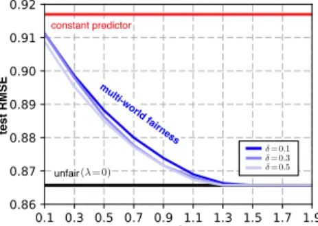
✏ te s t R MSE m ulti-w orld fa irn ess unfair constant predictor ( = 0) = 0.1 = 0.3 = 0.5
Figure 3:Test prediction results for differ-enton the law school dataset.
We begin by investigating a dataset of survey results across 163 U.S. law schools conducted by the Law School Admis-sion Council [19] . It contains information on over 20,000 students including their raceA(here we look at just black and white students as this difference had the largest effect in counterfactuals in [11]), their grade-point averageG obtained prior to law school, law school entrance exam scoresL, and their first year average gradeY. Consider that law schools may be interested in predictingY for all applicants to law school usingGandLin order to decide
whether to accept or deny them entrance. However, due to societal inequalities, an individual’s race may have affected their access to educational opportunities, and thus affectedGandL. Accordingly, we model this possibility using the causal graphs in Figure 2 (Left). In this graph we also model the fact thatG, Lmay have been affected by other unobserved quantities. However, we may be uncertain whether what the right way to model these unobserved quantities is. Thus we propose to model this dataset with the two worlds described in Figure 2 (Left). Note that these are the same models as used in Kusner et al. [11] (except here we consider race as the sensitive variable). The corresponding equations for these two worlds are as follows:
G=bG+wAGA+G G∼ N(bG+wGAA+wUGU, σG) (14) L=bL+wALA+L L∼Poisson(exp(bL+wLAA+wULU))
Y =bY +wYAA+Y Y ∼ N(wAYA+wYUU,1) G, L, Y ∼ N(0,1) U ∼ N(0,1)
where variablesb, ware parameters of the causal model.
Results. Figure 3 shows the result of learning a linear MWF classifier on the deterministic law school models. We split the law school data into a random 80/20 train/test split and we fit casual models and classifiers on the training set and evaluate performance on the test set. We plot the test RMSE of the constant predictor satisfying counterfactual fairness in red, the unfair predictor with λ= 0, and MWF, averaged across 5 runs. Here as we have one deterministic and one non-deterministic model we will evaluate MWF for differentandδ(with the knowledge that the only change in the MWF classifier for differentδis due to the non-deterministic model). For each, δ, we selected the smallestλacross a grid (λ∈ {10−510−4, . . . ,1010}) such that the constraint in eq. (6) held across
95%of the individuals in both models. We see that MWF is able to reliably sacrifice accuracy for fairness asis reduced. Note that as we changeδwe can further alter the accuracy/fairness trade-off.
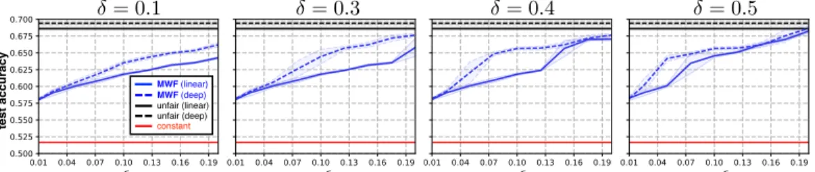
= 0.5 ✏ = 0.4 ✏ = 0.1 = 0.3 ✏ te s t a c c u ra c y ✏ MWF (linear) MWF (deep) constant unfair (linear) unfair (deep)
Figure 4: Test prediction results for differentandδon the COMPAS dataset. 4.2 Fair recidivism prediction (COMPAS)
We next turn our attention to predicting whether a criminal will re-offend, or ‘recidivate’ after being released from prison. ProPublica [13] released data on prisoners in Broward County, Florida who were awaiting a sentencing hearing. For each of the prisoners we have information on their raceA (as above we only consider black versus white individuals), their ageE, their number of juvenile feloniesJF, juvenile misdemeanorsJM, the type of crime they committedT, the number of prior offenses they haveP, and whether they recidivatedY. There is also a proprietary COMPAS score [13]Cdesigned to indicate the likelihood a prisoner recidivates.
We model this dataset with two different non-deterministic causal models, shown in Figure 2 (Right). The first model includes the dotted edges, the second omits them. In both models we believe that two unobserved latent factors juvenile criminalityUJand adult criminalityUDalso contribute to JF, JM, C, T, P. We show the equations for both of our casual models below, where the first causal model includes the blue terms and the second does not:
T ∼Bernoulli(φ(bT +wCUDUD+wECE+wCAA) (15) C ∼ N(bC+wCUDUD+wECE+wCAA+wCTT+wPCP+wCJFJF+wJMC JM, σC) P ∼Poisson(exp(bP+wUPDUD+wPEE+wAPA)) JF ∼Poisson(exp(bJF +w UJ JF +w E JFE+w A JFA)) JM ∼Poisson(exp(bJM+w UJ JM+w E JME+w A JMA)) [UJ, UD] ∼ N(0,Σ)
Results. Figure 4 shows how classification accuracy using both logistic regression (linear) and a 3-layer neural network (deep) changes as bothandδchange. We split the COMPAS dataset randomly into an 80/20 train/test split, and report all results on the test set. As in the law school experiment we grid-search overλto find the smallest value such that for anyandδthe(, δ)-ACF) constraint in eq. (6) is satisfied for at least95%of the individuals in the dataset, across both worlds. We average all results except the constant classifier over 5 runs and plot the mean and standard deviations. We see that for smallδ(high fairness) both linear and deep MWF classifiers significantly outperform the constant classifier and begin to approach the accuracy of the unfair classifier as increases. As we increaseδ(lowered fairness) the deep classifier is better able to learn a decision boundary that trades-off accuracy for fairness. But if, δis increased enough (e.g.,≥0.13, δ= 0.5), the linear MWF classifier matches the performance of the deep classifier.
5
Conclusion
This paper has presented a natural extension to counterfactual fairness that allows us to guarantee fair properties of algorithms, even when we are unsure of the causal model that describes the world. As the use of machine learning becomes widespread across many domains, it becomes more important to take algorithmic fairness out of the hands of experts and make it available to everybody. The conceptual simplicity of our method, our robust use of counterfactuals, and the ease of implementing our method mean that it can be directly applied to many interesting problems. A further benefit of our approach over previous work on counterfactual fairness is that our approach only requires the estimation of counterfactuals at training time, and no knowledge of latent variables during testing. As such, our classifiers offer a fair drop-in replacement for other existing classifiers.
6
Acknowledgments
This work was supported by The Alan Turing Institute under the EPSRC grant EP/N510129/1. CR acknowledges additional support under the EPSRC Platform Grant EP/P022529/1.
References
[1] Compas risk scales: Demonstrating accuracy equity and predictive parity performance of the compas risk scales in broward county, 2016. 2
[2] Julia Angwin, Jeff Larson, Surya Mattu, and Lauren Kirchner. Machine bias.https://www.propublica. org/article/machine-bias-risk-assessments-in-criminal-sentencing, 2016. Accessed: Fri 19 May 2017. 2
[3] Richard Berk, Hoda Heidari, Shahin Jabbari, Michael Kearns, and Aaron Roth. Fairness in criminal justice risk assessments: The state of the art.arXiv preprint arXiv:1703.09207, 2017. 1, 2
[4] Tim Brennan, William Dieterich, and Beate Ehret. Evaluating the predictive validity of the compas risk and needs assessment system.Criminal Justice and Behavior, 36(1):21–40, 2009. 1, 2
[5] A. P. Dawid. Causal inference without counterfactuals.Journal of the American Statistical Association, pages 407–448, 2000. 2
[6] Cynthia Dwork, Moritz Hardt, Toniann Pitassi, Omer Reingold, and Richard Zemel. Fairness through awareness. InProceedings of the 3rd Innovations in Theoretical Computer Science Conference, pages 214–226. ACM, 2012. 1
[7] Ian J. Goodfellow, Jean Pouget-Abadie, Mehdi Mirza, Bing Xu, David Warde-Farley, Sherjil Ozair, Aaron C. Courville, and Yoshua Bengio. Generative adversarial nets. InAdvances in Neural Information Processing Systems, pages 2672–2680, 2014. 1
[8] Amir E Khandani, Adlar J Kim, and Andrew W Lo. Consumer credit-risk models via machine-learning algorithms.Journal of Banking & Finance, 34(11):2767–2787, 2010. 1
[9] Keith Kirkpatrick. It’s not the algorithm, it’s the data.Communications of the ACM, 60(2):21–23, 2017. 2 [10] Jon Kleinberg, Sendhil Mullainathan, and Manish Raghavan. Inherent trade-offs in the fair determination
of risk scores.arXiv preprint arXiv:1609.05807, 2016. 2
[11] Matt J Kusner, Joshua R Loftus, Chris Russell, and Ricardo Silva. Counterfactual fairness.Advances in Neural Information Processing Systems, 31, 2017. 2, 4, 5, 8
[12] Moish Kutnowski. The ethical dangers and merits of predictive policing.Journal of Community Safety and Well-Being, 2(1):13–17, 2017. 2
[13] Jeff Larson, Surya Mattu, Lauren Kirchner, and Julia Angwin. How we analyzed the compas recidivism algorithm.ProPublica (5 2016), 2016. 9
[14] David Lopez-Paz. From dependence to causation.arXiv preprint arXiv:1607.03300, 2016. 2 [15] J. Pearl, M. Glymour, and N. Jewell.Causal Inference in Statistics: a Primer. Wiley, 2016. 2, 3 [16] Beth Pearsall. Predictive policing: The future of law enforcement.National Institute of Justice Journal,
266(1):16–19, 2010. 1, 2
[17] T.S. Richardson and J. Robins. Single world intervention graphs (SWIGs): A unification of the counter-factual and graphical approaches to causality.Working Paper Number 128, Center for Statistics and the Social Sciences, University of Washington, 2013. 2
[18] Paul Upchurch, Jacob Gardner, Kavita Bala, Robert Pless, Noah Snavely, and Kilian Weinberger. Deep feature interpolation for image content changes.arXiv preprint arXiv:1611.05507, 2016. 1
[19] Linda F Wightman. Lsac national longitudinal bar passage study. lsac research report series. 1998. 8 [20] Muhammad Bilal Zafar, Isabel Valera, Manuel Gomez Rodriguez, and Krishna P Gummadi. Fairness
beyond disparate treatment & disparate impact: Learning classification without disparate mistreatment.