Towards Efficient Hardware Acceleration of Deep Neural Networks on FPGA

(1)

TOWARDS EFFICIENT HARDWARE ACCELERATION OF

DEEP NEURAL NETWORKS ON FPGA

by

Sicheng Li

M.S. in Electrical Engineering,

New York University, 2013

B.S. in Electrical Engineering,

Beijing University of Posts and Communications, 2011

Submitted to the Graduate Faculty of

the Swanson School of Engineering in partial fulfillment

of the requirements for the degree of

Doctor of Philosophy

University of Pittsburgh

2017

(2)

UNIVERSITY OF PITTSBURGH

SWANSON SCHOOL OF ENGINEERING

This dissertation was presented

by

Sicheng Li

It was defended on

September 29 2017

and approved by

Hai (Helen) Li, Ph.D., Adjunct Associate Professor, Department of Electrical and Computer

Engineering

Yiran Chen, Ph.D., Adjunct Associate Professor, Department of Electrical and Computer

Engineering

Zhi-Hong Mao, Ph.D., Associate Professor, Department of Electrical and Computer Engineering

Ervin Sejdic, Ph.D., Associate Professor, Department of Electrical and Computer Engineering

Yu Wang, Ph.D., Associate Professor, Department of Electrical Engineering, Tsinghua University

Dissertation Director: Hai (Helen) Li, Ph.D., Adjunct Associate Professor, Department of

(3)

Copyright cby Sicheng Li 2017

(4)

TOWARDS EFFICIENT HARDWARE ACCELERATION OF

DEEP NEURAL NETWORKS ON FPGA

Sicheng Li, PhD

University of Pittsburgh, 2017

Deep neural network (DNN) has achieved remarkable success in many applications because of its powerful capability for data processing. Their performance in computer vision have matched and in some areas even surpassed human capabilities. Deep neural networks can capture complex non-linear features; however this ability comes at the cost of high computational and memory require-ments. State-of-art networks require billions of arithmetic operations and millions of parameters. The brute-force computing model of DNN often requires extremely large hardware resources, in-troducing severe concerns on its scalability running on traditional von Neumann architecture. The well-known memory wall, and latency brought by the long-range connectivity and communica-tion of DNN severely constrain the computacommunica-tion efficiency of DNN. The acceleracommunica-tion techniques of DNN, either software or hardware, often suffer from poor hardware execution efficiency of the simplified model (software), or inevitable accuracy degradation and limited supportable algorithms (hardware), respectively. In order to preserve the inference accuracy and make the hardware im-plementation in a more efficient form, a close investigation to the hardware/software co-design methodologies for DNNs is needed.

The proposed work first presents an FPGA-based implementation framework for Recurrent Neural Network (RNN) acceleration. At architectural level, we improve the parallelism of RNN training scheme and reduce the computing resource requirement for computation efficiency en-hancement. The hardware implementation primarily targets at reducing data communication load. Secondly, we propose a data locality-aware sparse matrix and vector multiplication (SpMV) kernel. At software level, we reorganize a large sparse matrix into many modest-sized blocks by

(5)

adopt-ing hypergraph-based partitionadopt-ing and clusteradopt-ing. Available hardware constraints have been taken into consideration for the memory allocation and data access regularization. Thirdly, we present a holistic acceleration to sparse convolutional neural network (CNN). During network training, the data locality is regularized to ease the hardware mapping. The distributed architecture enables high computation parallelism and data reuse. The proposed research results in an hardware/soft-ware co-design methodology for fast and accurate DNN acceleration, through the innovations in algorithm optimization, hardware implementation, and the interactive design process across these two domains.

(6)

3.0 THE RECONFIGURABLE SPMV KERNEL . . . 27

3.1 Preliminary . . . 27

3.1.1 Sparse Matrix Preprocessing . . . 27

3.1.2 The Existing SpMV Architectures . . . 28

3.2 Design Framework . . . 29

3.3 Sparse Matrix Clustering . . . 32

3.3.1 Workload Balance . . . 32

3.3.2 Hardware-aware Clustering . . . 34

3.3.3 Strong Scaling vs. Weak Scaling . . . 35

3.3.4 Hardware Constraints. . . 36

3.4 Hardware Implementation . . . 37

3.4.1 Global Control Unit (GCU) . . . 37

3.4.2 Processing Element (PE) . . . 39

3.4.3 Thread Management Unit (TMU) . . . 39

3.4.4 Hardware Configuration Optimization . . . 41

3.5 Evaluation . . . 42

3.5.1 Experimental Setup . . . 42

3.5.2 System Performance . . . 44

3.5.3 The Impact of Data Preprocessing . . . 46

3.5.4 Comparison to Previous Designs . . . 49

3.6 Conclusions . . . 49

4.0 SPARSE CONVOLUTIONAL NEURAL NETWORKS ON FPGA . . . 51

4.1 Introduction . . . 51

4.2 CNN Acceleration and Difficulty . . . 53

4.2.1 Dense CNN Acceleration. . . 53

4.2.2 Inefficient Acceleration of Sparse CNN . . . 54

4.3 The Proposed Design Framework . . . 55

(8)

4.4.1 Locality-aware Regularization . . . 58

4.4.2 Sparse Network Representation . . . 60

4.4.3 Kernel Compression and Distribution . . . 62

4.5 Hardware Implementation . . . 65

4.5.1 The System Architecture . . . 65

4.5.2 The PE Optimization . . . 66

4.5.3 Zero Skipping for Computation Efficiency. . . 68

4.5.4 Data Reuse to Improve Effective Bandwidth . . . 69

4.6 Hardware Specific Optimization . . . 69

4.6.1 Design Trade-offs on Cross Layer Sparsity . . . 70

4.6.2 Hardware Constraints. . . 71

4.7 Evaluation . . . 72

4.7.1 Experimental Setup . . . 72

4.7.2 Layer-by-Layer Performance . . . 73

4.7.3 End-to-End System Integration. . . 75

4.8 Conclusions . . . 77

5.0 RELATED WORK . . . 79

6.0 CONCLUSION AND FUTURE WORK . . . 83

(9)

LIST OF TABLES

1 RNN Computation Runtime Breakdown in GPU . . . 10

2 Memory Access Requirement . . . 16

3 Resource Utilization . . . 21

4 Accuracy Evaluation on MSRC . . . 22

5 Configuration of Different Platforms . . . 22

6 Runtime (in Seconds) of RNNLMs with Different Network Size . . . 23

7 Power Consumption . . . 24

8 Computation Engine Efficiency . . . 25

9 Resource Utilization . . . 42

10 Characteristics of Benchmarks . . . 43

11 Configuration and System Performance of Different Platforms . . . 44

12 System Properties for Previous Implementations and This Work . . . 48

13 The average weight sparsity and accuracy of three selected CNN models after reg-ularization. . . 60

14 The average sparsity and replication rate of the input feature maps of Conv layers in AlexNet. . . 67

15 Configuration of different platforms . . . 72

16 Resource utilization on FPGA . . . 73

17 Performance evaluation on sparse Conv and FC Layers of AlexNet on ImageNet . . 74

(10)

LIST OF FIGURES

1 (a) Feedforward neural network; (b) Recurrent neural network. . . 7

2 Unfold RNN for training through BPTT algorithm. . . 9

3 The system speedup is saturated with the increment of CPU cores as the memory accesses become the new bottleneck. . . 11

4 The data flow of a two-stage pipelined RNN structure [1]. The computation com-plexity of white boxes in output layer is much bigger than that of gray boxes in hidden layer. . . 12

5 Our proposed parallel architecture for RNNLM. . . 13

6 The impact of the reduced data precision ofWho in RNNLM on the reconstruction quality of word sequences. . . 14

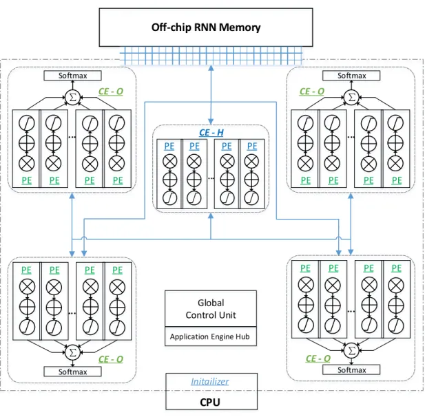
7 An overview of the RNNLM hardware implementation. . . 15

8 The thread management unit in a computation engine. PEs are connected through a crossbar to the shared memory structure. . . 17

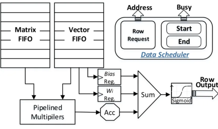
9 The multi-thread based processing element. . . 18

10 An example of compressed row storage (CSR). . . 28

11 The sparsity affects SpMV performance. . . 29

12 Our proposed data locality-aware design framework for SpMV acceleration. . . 31

13 Applying the partitioning and clustering on a sparse matrix (lns 3937). . . 33

14 The performance penalty brought by inter-PE communications. . . 36

15 The architecture for SpMV acceleration. . . 38

16 Configuration header file is used to schedule inter-PE communication.. . . 38

(11)

18 Hardware constraint analysis by varying the size of input matrix/PE. . . 41

19 System performance on selected benchmarks. . . 45

20 The analysis on the data preprocessing. . . 47

21 Our evaluation on AlexNet sparsity and speedup. Conv1 refers to convolutional

layer 1, and so forth. The baseline is profiled by GEMM of Caffe. The sparse kernel weights are stored in compressed sparse row (CSR) format and accelerated

by cuSPARSE. . . 52

22 The impact of kernel matrix sparsity on convolution performance. . . 54

23 Our proposed SW/HW co-design framework for CNN sparsification & acceleration

on FPGA.. . . 56

24 Kernel weights are split into pre-defined groups. A compact kernel is obtained

through the locality-aware regularization. . . 58

25 The locality-aware regularization first imposes sparsity on a pre-trained dense AlexNet,

fine-tuning is applied to retain accuracy. . . 59

26 An illustration of our proposed sparse network representation for sparse CNN

ac-celeration. . . 61

27 Locality-aware regularization on Conv layer. . . 63

28 Our string-based compression balances computation and memory, showing a strong

scalability. . . 64

29 The system architecture overview of the FPGA-based sparse CNN accelerator. . . . 65

30 The address access pattern during matrix multiplication within one PE. . . 66

31 The data reuse pattern of feature map. . . 68

32 The trade-off between computation requirement (a) and model size (b) under

dif-ferent sparse regularization on Conv and FC layers of AlexNet. Conv 1 with low

sparsity is omitted in (b). . . 70

33 The performance is evaluated by applying the proposed optimizations and compared

with the dense model. The sparse model is compressed first, then adds zero skipping

and data fetcher, respectively. . . 75

34 Accelerator performance on different network structures. The speedup ratio is

(12)

35 Volta GV100 Tensor Core operation. . . 80

36 The layout of DianNao [2]. . . 81

(13)

1.0 INTRODUCTION

Following technology advances in high performance computation systems and fast growth of data acquisition, machine learning, especially deep learning, made remarkable success in many research areas and applications, such as image recognition [4], object detection [5], natural language pro-cessing [6] and automatic speech recognition [7]. Such a success, to a great extent, is enabled by developing large-scale deep neural networks (DNN) that learn from a huge volume of data. For example, inLarge Scale Visual Recognition Challenge 2012, Krizhevsky et al. beat out the second-best team 10% in Imagenet classification accuracy by training a deep convolutional neural network with 60 million parameters and 650,000 neurons on 1.2 million images. The deployment of such a big model is both computation-intensive and memory-intensive. At software level, ex-tending the depth of neural networks for accuracy optimization becomes a popular approach [8][9], exacerbating the demand for computation resources and data storage of hardware platforms.

The research on hardware acceleration for neural network has been extensively studied on not only the general-purpose platforms, e.g., graphic processing units (GPUs), but also domain-specific hardware such as field-programmable gate arrays (FPGAs) and custom chip (e.g., TrueNorth) [10][11][12][13][14]. High-end GPUs enable fast deep learning, thanks to their large through-put and memory capacity. When training AlexNet with Berkeley’s deep learning framework Caffe ([10]) and Nvidia’s cuDNN ([15]), a Tesla K-40 GPU can process an image in just 4ms. While GPUs are an excellent accelerator for deep learning in the cloud, mobile systems are much more sensitive to energy consumption. In order to deploy deep learning algorithm in energy-constraint mobile systems, various approaches have been offered to reduce the computational and memory requirements of deep neural networks).

(14)

1.1 DEEP NEURAL NETWORKS ON FPGAS

Field Programmable Gate Arrays (FPGAs) have shown massive speedup potential for a wide range of applications. Their ability to support highly parallel designs, coupled with their re-programmability have made them very attractive platforms. Custom pipelined datapaths allow the FPGA to execute in parallel what could take thousands of operations in software. Programmabil-ity, and ease of use deter many software developers from expanding into hardware development. FPGAs are notorious for complex designs, long debug cycles, and difficult verification among other things. However, some of these issues can be alleviated by advances in hardware design tools. Major FPGA manufactures are actively developing High Level Synthesis (HLS) tools to help software software developers utilize their boards. Besides, FPGAs now have easy access to significantly larger memory spaces, which allows researchers to consider much larger real-world problems. However, the larger memories come at a cost of higher latencies.

Various FPGA-based DNN accelerators ([16][17]) have proven that it is possible to use recon-figurable hardware for end-to-end inference of large CNNs like AlexNet and VGG. An important problem faced by designers of FPGA-based DNNs is to select the appropriate DNN model for a specific problem to be implemented using optimal hardware resources. Moreover, the progress of hardware development still falls far behind the upscaling of DNN models at software level. With the high demand for computation resources, memory wall [14] that describing the disparity be-tween fast on-chip data processing rate and slow off-chip memory and disk drive I/O demonstrates more prominent adverse impact [18][19].

1.2 DISSERTATION CONTRIBUTION AND OUTLINE

To overcome the above challenges in neural network acceleration, both hardware and software solutions are investigated. The software approaches, in contrast, mainly concentrate on reducing the scale and connections of a DNN model while still keeping the state-of-the-art accuracy. The hardware approaches attempt to build a specialized architecture for the customized network models adapting to it.

(15)

Our proposed work can be decoupled as following two main research scopes: 1) FPGA accel-eration of recurrent neural network based language model; 2) A data locality-aware design frame-work for reconfigurable sparse matrix-vector multiplication kernel. 3) The software-hardware co-design on sparse convolutional neural networks.

For research scope 1, we proposed an FPGA-based acceleration for recurrent neural networks, which includes three major technical contributions:

• At architectural level, the framework extends the inherent parallelism of RNN and adopts a mixed-precision scheme. The approach enhances the utilization of configurable logics and improves computation efficiency.

• The hardware implementation integrates a groups of computation engines and a multi-thread management unit. The structure successfully conceals the irregular memory access feature in data back-propagation stage and reduces external memory accesses. Our framework is de-signed in a scalable manner to benefit the future investigation for ever-larger networks.

We realized the RNNLM on Convey HC-2ex system. The design was trained with a dataset of 38Mwords. It consists of1,024nodes in hidden layer. Our design performs better than traditional class-based modest-size recurrent networks and obtains 46.2% in accuracy inMicrosoft Research

Sentence Completion(MRSC) challenge. The experiments at different network sizes on average

achieve 14.1× speedup over the optimized CPU implementation and a comparable performance with high-end GPU system, demonstrating a great system scalability.

For research scope 2, we developed an efficient SpMV computation kernel for sparse neural networks. The main contributions of this work are:

• By analyzing the impact of the sparse structure of matrix and various hardware parameters on system performance and accordingly propose a data locality-ware co-design framework for iterative SpMV.

• We integrate conventional sparse matrix compression formats with a locality-aware clustering technique. A sparse matrix will be reorganized into sub-blocks, each of which has regularized memory accesses. At hardware level, we develop a scalable architecture made of high-parallel processing elements (PEs) that enable simultaneous MACs and customized data path for inter-PE communications.

(16)

The experiments based on the University of Florida sparse matrix collection shows dramatic im-provement in computational efficiency. Our FPGA-based implementation has a comparable run-time as GPU and achieves 2.3× reduction than CPU, with substantial saving in power consump-tion, say,8.9×and8.3×better than the implementations on CPU and GPU, respectively.

To enable the CNN sparsification and acceleration on FPGA, for both convolutional and fully connected layers within CNNs, we propose a co-design framework by combining innovations in software and hardware domains. More specific, the main contributions of this work include:

• We profile the impact of sparse network structures and hardware parameters on overall system performance and demonstrate that the software/hardware co-design is necessary to accelerate sparse CNNs.

• At software level, we focus on the data locality enhancement during model sparsification. Alone with a low-cost compression scheme, kernel weights are partitioned into sub-blocks with regularized data layout. At hardware level, a scalable architecture composed of processing elements (PEs) that simultaneously execute compressed kernel weights is developed. Zero-skipping and extensive data reuse scheme are applied to improve the operation efficiency of sparse feature map.

• As the sparse regularization affects the connections over layers, we introduce a sparsi

cation strategy which can adapt the design optimization according to the available hardware resource.

We evaluate the proposed design framework through three representative CNNs on two Xilinx FPGA platforms - ZC706 and VC707 boards. Our design can significantly improve the computa-tion efficiency and effiective memory bandwidth, achieving an average 67.9% of the peak perfor-mance. This result is 1.8× and4.7× higher than that of the implementations on high-end CPUs and GPUs, respectively. Very importantly, our design effectively reduces the classification time 2.6×, compared to state-of-the-art FPGA implementation.

The outline of this dissertation is organized as follows: Chapter1presents the overall picture of this dissertation, including the research motivations, research scopes and the research contri-butions; The details and applications of our acceleration framework for recurrent neural networks are illustrated in Chapter2. Then, the sparse matrix-vector computation kernel will be presented

(17)

in Chapter 3. Chapter 4 demonstrates the benefits of our proposed software-hardware co-design framework, and its evaluation result on sparse convolutional neural networks. Chapter 6 finally summarizes the research work and presents the potential future research directions, as well as our insights for efficient acceleration of deep neural networks on FPGA.

(18)

2.0 FPGA ACCELERATION TO RNN-BASED LANGUAGE MODEL

In this chapter, we will present the details of our hardware acceleration framework for recurrent neural network-based language model. The structure of this chapter is organized as the follows: Section2.1introduces the language model and RNN algorithm; Section2.2presents our analytical approach for accelerator design optimization; Section2.3and2.4explain our proposed architecture and the corresponding hardware implementation, respectively; Experimental results and analysis are shown in Section2.5.

2.1 PRELIMINARY

2.1.1 Language Models

Rather than checking linguistic semantics, modern language models based on statistical analy-sis assign a probability to a sequence of words by means of a probability distribution. Ideally, a meaningful word sequence expect to have a larger probability than an incorrect one, such as

P(I saw a dog)> P(Eye saw a dog).

Among developed language models,n-gram modelis the most commonly used. In an n-gram model, the probability of observing the ith wordwi in the context history of the precedingi−1 words can be approximated by the probability of observing it in the shortened context history of the precedingn−1words. For example, in a2-gram(also called asbigram) model, the probability of “I saw a dog” can be approximated as:

P(I saw a dog) =P(I|−)×P(saw|I)×P(a|saw) ×P(dog|a)×P(−|dog)

(19)

A conditional probability,e.g.,P(a|saw)in Eq. (2.1), can be obtained through statistical anal-ysis based on training data. The number of conditional probabilities required in n-gram increases exponentially as n grows: for a vocabulary with a size of V, an n-gram model need store Vn parameters. Moreover, the space of training data becomes highly sparse asn increases. In other words, a lot of meaningful word sequences will be missed in the training data set and hence sta-tistical analysis cannot provide the corresponding conditional probabilities. Previous experiments showed that the performance of n-gram language models with a larger n (n > 5) is less effec-tive [20]. N-gram model can realize only the short-term perspective of a sequence, which is clearly insufficient to capture semantics of sentences [21].

2.1.2 RNN & RNN based Language Model

Figure1illustrates the structure of a standardrecurrent neural network(RNN). Unlike feedforward neural networks where all the layers are connected in a uniform direction, a RNN creates additional recurrent connections to internal states (hidden layer) to exhibit historical information. At timet, the relationship of input ~x(t), the temporary state of hidden layer~h(t), and output ~y(t) can be described as ~h(t) = fWih~x(t) +Whh~h(t−1) +~bh , and (2.2) ~ y(t) =g Who~h(t) +~bo . (2.3) Hidden O utp ut Inp ut Hidden O utp ut Inp ut

(20)

Where,Wih is the weight matrix connecting the input and hidden layers,Who is the one between the hidden and output layers. Whhdenotes the recurrent weight matrix between the hidden states at two consecutive time steps, e.g.,~h(t−1)and~h(t). ~bh and~bo are the biases of the hidden and output layers, respectively. f(z)andg(z)denote the activation functions at the hidden and output layers, respectively.

The input/output layer of RNN-based language model (RNNLM) corresponds to the full or compressed vocabulary. So each node represents one or a set of words. In calculating the prob-ability of a sentence, the words will be input in sequence. For instance, ~x(t)denotes the word at timet. And output~y(t)represents the probability distribution of the next word, based on~x(t)and the historical information stored as the previous state of network~h(t−1).

RNNLM uses internal states at hidden layer to store the historical information, which is not constrained by the length of input history. Compared with n-gram models, RNNLM is able to realize a long-term perspective of the sequence. Note that the hidden layer usually has much less nodes than the input/output layer and its size shall reflect the amount of training data: the more training data are collected, the larger hidden layer is required. Moreover, the aforementioned sparsity of the training data in n-gram language model is not an issue in RNNLM, indicating that RNNLM has a stronger learning ability [22].

2.1.3 The RNN Training

When training a network of RNNLM, all data from training corpus are presented sequentially. In this work, we usedback-propagation through time(BPTT) algorithm. As illustrated in Figure 2, the approach truncates the infinite recursion of a RNN and expands it to a finite feed-forward structure, which then can be trained by following the regular routine of feed-forward networks.

For a given input data, the actual output of network shall first be calculated. Then the weights of each matrix will be updated through back-propagating the deviations between the actual and desired outputs layer by layer. The update of weightwji between node iof the current layer and nodej of the next layer at timetcan be expressed as wji ← wji+η·

T

P

t=1

δj(t)·xi(t),wherexi(t) is the input of nodei;ηis the learning rate;δj(t)is the error back-propagated from nodej; andT is the BPTT step for RNN training.

(21)

Hidden (State)

Input Output

t - 1

t

t + 1

Figure 2: Unfold RNN for training through BPTT algorithm.

At the output layer, we adoptedsoftmaxactivation functiong(z) = Pez

kezk as the cross-entropy

loss function. The error derivative of node p δp(t) can be obtained simply from RNN’s actual outputop(t)and the desired onetp(t):

δp(t) =tp(t)−op(t). (2.4)

Sigmoidfunctionf(z) = ₁₊1_e−z is utilized at the hidden layer. The error derivative of nodek

δk(t)is calculated by

δk(t) = f0(x)|f(x)=hk(t)·δBPTT(t). (2.5)

Where,hk(t)is the state of nodekin hidden layer at timet. δBPTTis the accumulation of the errors back-propagated through time, that is,

δBPTT(t) = X o∈output wokδo(t) + X h∈hidden whkδh(t+ 1). (2.6)

Here,δo(t)denotes the error of output layer at timet, whileδh(t+ 1)is the error of hidden layer back-propagated from the following time step t+ 1. w_ok andw_hk are the transposed weights of

(22)

2.2 ANALYSIS FOR DESIGN OPTIMIZATION

We first analyze the utilization of computation and communication resources in RNNLM as these are two principal constraints in system performance optimization.

Computation resource utilization. To analyze the computation cost, we implemented RNNLM

on a CUBLAS-based NVIDIA GPU and profiled the runtime of every major function. The result in Table 1 shows that the matrix-vector multiplication consumes most of computation resource. The activation functions, as the second contributor, consume more than 20% of runtime. So we mainly focus on enhancing the computation efficiency of these two functions.

Memory accesses. During training, the matrix-vector multiplication in the back-propagation

phase requires the transposed form of weight matrices as shown in Eq. (8). Such a data access exhibits irregular behavior, making the further performance improvement very difficult. To explore this effect experimentally, we mapped RNNLM on a multi-core server with Intel’s Math Kernel

Library(MKL). Figure3shows the normalized system performance. As more cores are utilized,

the major constrain changes from computation resource to memory bandwidth. Accordingly, the speedup becomes slower and eventually saturated when the memory bandwidth is completed con-sumed.

Scalability. A scalable implementation must well balance the use of computation units and

memory bandwidth. As the configurable logic elements on FPGA grow fast, the implementation shall be able to integrate additional resources. Our approach is to partition a design into multiple identical groups and migrate the optimized development of a group to bigger and ore devices for applications in larger scale.

Table 1: RNN Computation Runtime Breakdown in GPU

Matrix-vector Activation Sum of Vector

Delta Others Multi. Functions Vector Elem. Scaling

(23)

0.5 1.5 2.5 3.5 0 4 8 12 16 20 24 S pe ed -u p R a ti o Number of Cores Actual Ideal

Figure 3: The system speedup is saturated with the increment of CPU cores as the memory accesses become the new bottleneck.

2.3 ARCHITECTURE OPTIMIZATION

This section describes the optimization details at the architectural level. We propose a parallel architecture to improve the execution speed between the hidden and output layers. Moreover, the computation efficiency is enhanced by trading off data and function precision.

2.3.1 Increase Parallelism between Hidden and Output Layers

Previously, Liet al. proposed a pipeline architecture to improve the parallelism of RNN [1]. As illustrated in Figure4, it partitions the feed-forward phase into two stages: the data flow from input to hidden layer represented by gray boxes and the computation from hidden to output layer denoted in white boxes. Furthermore, it unfolds RNN along time domain by tracingB previous time steps (usually2∼10) and pipelines these calculations.

However, our analysis reveals that the two stages have extremely unbalanced throughputs. Assume a RNN withV nodes in the input and output layers andHnodes in the hidden layer. The input layer activates only one node at a time, soWih~x(t)in Eq. (3) can be realized by extracting the row ofWihcorresponding to the activated node, that is, copying a row ofWihto the destination vector. Thus, the computation complexity of~h(t)is mainly determined byWhh~h(t−1), which is

(24)

{Whh·h(t-1) +bh +Wih·

x

(t-1)}sigmoid {Who

·

h(t) +bo }softmax

y(t)

Computation Complexity

h(t-1)

h(t)

Hidden Layer Output Layer

see Eq. (3) see Eq. (4)

h(t)

Hidden Layer ~ (H × H)

~ (H × V) h(t+1)

Figure 4: The data flow of a two-stage pipelined RNN structure [1]. The computation complexity of white boxes in output layer is much bigger than that of gray boxes in hidden layer.

dominant. UsuallyV is related to the vocabulary and can easily reach up to a size of10K∼200K while H can maintain at a much smaller scale like 0.1K ∼1K. Thus, the execution time of the second stage is much longer than that of the first one. Such a pipelined structure [1] is not optimal for the entire workload.

Our effort is dedicated in further improving the execution of the second stage. As illustrated in Figure 5, we duplicate more processing elements of the output layer. More specific, our pro-posed architecture conducts the calculation of the hidden layer in serial while parallelizing the computation of the output layer. For example, assumeB is 4. At time stept−3, the result of the hidden layer goes toOutput Layer I. WhileOutput Layer Iis in operation att−2, the hidden layer will submit more data to the next available output layer processing element, e.g.,Output Layer II. As such, the speed-up ratio of the proposed design over the two-stage pipelined structure can be approximated by

Speed-up= (tV +tH) +tV ×(B−1)

tH ×B +tV

, (2.7)

where tV and tH are the latencies of the output layer and the hidden layer, respectively. For instance, assumeV= 10K,H= 0.1K, andB= 4, the execution of our architecture is about3.86× faster than the design of [1].

(25)

Output Layer II Output Layer I

Output Layer III Output Layer IV

x(t-3), x(t-2), x(t-1), x(t) h(t-2) h(t-3) h(t) h(t-1) y(t-2) y(t-3) y(t) y(t-1) Hidden Layer

Figure 5: Our proposed parallel architecture for RNNLM.

For the proposed design,Bshall be carefully selected based upon application’s scale. From the one hand, a biggerB indicates more time steps processed in one iteration and therefore requires more resources. From the other hand, the higherBis, the faster execution can be obtained. More-over, by introducing more time steps, more historic information are sustained for better system accuracy too.

2.3.2 Computation Efficiency Enhancement

Through appropriately trading off data and function precision of RNNLM, we can greatly improve its computation efficiency without degrading the training accuracy.

Fixed-point data conversion. The floating-point data are adopted in the original RNNLM

al-gorithm and the corresponding hardware implementation, which demand significant computation resources and on-chip data space. The fixed-point operation is more efficient in FPGA implementa-tion but the errors caused by precision truncaimplementa-tion could accumulate iteratively. Fortunately, neural networks exhibit self-recovery characteristics, which refers to the tolerance to noise in decision making.

Mixed-precision data format. As the computation of output layer is more critical, lowering the

data precision ofWho, if possible, would be the most effective option. We analyze RNNLM using the Fixed-Point MATLAB Toolbox and evaluate the quality of different data format by examining

(26)

6 7 8 9 10 11 12 13 14 15 16 17 18 P er p lex it y (P P L) Coefficient width Fixed Point Floating Point

Figure 6: The impact of the reduced data precision ofWhoin RNNLM on the reconstruction quality of word sequences.

and keep the other training parameters as well as the states of hidden and output layers in original 64 bits, a fixed-point implementation can achieve the same reconstruction quality as a floating-point design. In other words, this scheme improves the runtime performance while maintaining the system accuracy to the maximum extent.

Approximation of activation functions. Our preliminary investigation in Table 1 reveals that

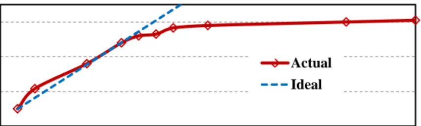
the activation functions are the second contributor in runtime. This is because the complex oper-ations in sigmoidandsoftmaxfunctions, such as exponentiation and division (Section2.1.3), are very expensive in hardware implementation. Instead of precisely mapping these costly operations to FPGA, we adopt thepiecewise linear approximation of onlinear function(PLAN) [23] and sim-plify the activation functions with the minimal number of additions and shifts. Our evaluation shows that on average, the error between our approximation and the real sigmoid calculation is only 0.59%, which doesn’t affect much on the convergence properties in RNNLM training.

2.4 HARDWARE IMPLEMENTATION DETAILS

The hardware implementation in FPGA will be presented in this section. We map the proposed architecture tocomputation engines(CEs), each of which is divided into a fewprocessing elements

(27)

2.4.1 System Overview PE PE PE PE ... PE PE PE PE ... Off-chip RNN Memory PE ... PE PE PE ∑ Softmax PE PE PE PE ... ∑ Softmax ∑ Softmax PE PE PE PE ... ∑ Softmax Global Control Unit Application Engine Hub

CPU Initailizer CE - O CE - H CE - O CE - O CE - O

Figure 7: An overview of the RNNLM hardware implementation.

Figure 7presents an overview of our hardware implementation on the Convey HC-2ex com-puter system. The CPU on the host side is used for accelerator startup and weight initialization. There are 16 DIMMs and 1024 banks in the off-chip memory. Thus the chance of bank conflicts is low even the parallel accesses are random. The global control unit receives commands and configuration parameters from the host throughapplication engine hub(AEH).

We map the proposed parallel architecture of RNNLM into two types ofcomputation engines

(28)

and multiple CE-O are required. The two types of CEs are customized for high efficiency, with the only difference in the design of activation function. The system configuration,e.g., the number and scale of CEs, is upon users’ decision. Moreover, each CE is segmented into several identical

processing elements(PEs). Since the major of RNNLM execution is performed through these PEs,

the proposed implementation can easily be migrated to a future device by instantiating more PEs. The matrix-vector multiplication not only consumes the most runtime but also demands a lot of data exchange as shown in Table 2. The situation in the feed-forward phase can be partially alleviated by data streaming and datapath customization. However, the multiplication operations of transposed matrices in the back-propagation phase exhibit very poor data locality, leading to nontrivial impact on memory requests. The long memory latencies potentially could defeat the gains from parallel executions. In addition, Table 2 implies that the data accesses in RNNLM have very diverse characteristics, each of which shall be considered specifically in memory access optimizations. These details will be presented in the following subsections.

2.4.2 Data Allocation

From the one hand, the RNNLM implementation is associated with an extremely large data set, including a training data set (e.g., 38Mwords in our test) as well as the weight parameters (e.g., 40Mbfor a vocabulary of10Kwords and the hidden layer of1Knodes). From the other hand, only a small amount of index data are required to control the RNNLM training process: at a time step,

Table 2: Memory Access Requirement

Dataset Operation Total # Size (byte)

Training data read only 38M 152M

Wih,Who read & write V×H(10K×1K) 40M

Whh read & write H×H(1K×1K) 4M

bo,~y(t) read & write V (10K) 40K

(29)

PE

0

PE

1

PE

N-1

PE

N

mc 0 mc 1 mc 2 mc 3 mc 4 mc 5 mc 6 mc 7

...

SDRAM SDRAM SDRAM SDRAM SDRAM SDRAM SDRAM SDRAM SDRAM SDRAM SDRAM SDRAM SDRAM SDRAM SDRAM SDRAM

Thread Management Unit

Computation Engine

Figure 8: The thread management unit in a computation engine. PEs are connected through a crossbar to the shared memory structure.

only one input node will be activated and only one output node will be monitored. Therefore, we propose to store the training data in the host main memory and feed them into the FPGAs during each training process.

Though FPGA in the Convey HC-2exsystem (Xilinx Virtex6 LX760) has a large on-chip block RAM (about 26MB), not all the space is available for users. Part of it is utilized for interfacing with memory and other supporting functions. Therefore, we keep the intermediate data which are frequently access and update in the training process, such as all the parameters (Wih, Whh, Who,

bh, andbo) and all the states of hidden and output layers, in the off-chip memory instead of on-chip memory. Only a subset of data is streamed into the limited on-chip memory at runtime for the best utilization and system performance.

2.4.3 Thread Management in Computation Engine

How to increase the effective memory bandwidth is critical in CE design. Previously, Ly and Chow proposed to remove the transpose of a matrix by saving all the data in on-chip block RAMs [24]. At a time, only one element per row/column of the matrix is read out through a carefully designed addressing scheme. As such, a column or row of the matrix is obtained from one memory thread.

(30)

Pipelined Multipilers Start End Row Request Acc Bias Reg. Wi Reg. Sum Matrix FIFO Vector FIFO Address Busy Sigmoid Row Output Data Scheduler

Figure 9: The multi-thread based processing element.

However, the approach requires that the weight matrix fits on-chip memory and the number of block RAMs for the weight matrix equals to the number of neurons in different layers. It is not applicable to our RNNLM in a much larger scale.

There are 16 channels in the system. To improve the memory efficiency, we introduce a hard-ware supported multi-threading architecture named asthread management unit (TMU). Figure8

illustrates its utilization in CEs. To process all the elements of a matrix row through a single memory channel, TMU generates a thread for each matrix row and the associated start and end conditions. All the ready threads are maintained by TMU. Once a channel finishes a row, it can switch to another ready tread, which usually has been prefetched from memory so the memory la-tency is masked. Each PE holds abusyflag high to prevent additional threads from being assigned. When all the PEs are busy, TMU backloads threads for later assignment.

TMU supports the data communication among a large number of PEs and improves the execu-tion parallelism. Note that there is only one TMU in a CE. Increasing the number of PEs does not introduce more hardware overhead.

(31)

Algorithm 1Data flow from input layer to hidden layer 1: fort = 0;t < BP T T;t+ + do

2: ift!= 0then

3: mvmulti(Whh,hidden(t−1),hidden(t)); 4: vdadd(hidden(t),bh,h(t)); 5: vdadd(hidden(t),w~k ih,hidden(t)); 6: else 7: vddadd(w~k ih,bh,hidden(t)); 8: end if

9: sigmoid(hidden(t),hidden(t)); 10: end for

2.4.4 Processing Element Design

The computation task within a CE is performed through processing elements (PEs). These PEs operate independently, each of which takes charge of a subset of the entire task. For example, when realizing a matrix-vector multiplication, each PE is assigned with a thread that computes a new vector value based on a row of the weight matrix. Data transition can operate in the burst mode: based on the start and end addresses, a thread fetches all the requested data in a row from the off-chip memory, as shown in Figure9.

CE controls the memory requests of the weight matrix and vector arrays. The Convey system supports the in-order return of all memory requests, so the reordering of memory accesses can be done through TMU assisted by the crossbar interface from FPGAs to memory modules. Data returned from memory can be buffered inMatrix and Vector FIFOs, using the corresponding thread id as the row index. When a new thread is assigned to a PE, it raises abusyflag and requests the weight and vector data from memory based on the start and end addresses. Once all the memory requests for the thread are issued, the flag isreset, indicating that the PE is ready for another thread even through the data of the prior thread is still in processing. As such, the memory access load can be dynamically balanced across all PEs.

(32)

2.4.5 Data Reuse

Off-chip memory accesses take long time. For example, the memory latency on our Convey plat-form is 125 cycles at 150MHz. To speed up the execution of RNNLM, we can reduce off-chip memory accesses through data reuse.

Algorithm 1 presents the data flow from input to hidden layer, during which the state of hidden layer is frequently accessed. Similar data access pattern has also been observed in the calculation of output layer. We propose reuse buffers for matrix and bias vector respectively named asWi Reg.

andBias Reg. as shown in Figure9. First, a row of weight matrix are fed into an array of multipliers

that are organized in fine-grain pipeline and optimized for performance. While data goes into the accumulator and completes the matrix multiplication, the weight and bias are buffered registers. After data summation is completed, PE enables its activation function, e.g., sigmoid in CE-H or

softmaxinCE-O, to obtain the state of hidden/output layer.

2.5 EXPERIMENTAL RESULTS

In this section, we present the experimental results of the RNNLM implementation and evalu-ate the proposed framework in terms of training accuracy, system performance, and efficiency of computation engine design.

2.5.1 Experiment Setup

We implemented the RNNLM on the Convey HC-2ex _{platform [}₂₅_{]. We described the design in} System C code, which then was converted to Verilog RTL using Convey Hybrid Threading HLS tool ver. 1.01. The RTL is connected to memory interfaces and the interface control is provided by Convey PDK. Xilinx ISE 11.5 is used to obtain the final bitstream. Table 3 summarizes the resource utilization of our implementation on one FPGA chip. The chip operates at150MHzafter placement and routing.

(33)

2.5.2 Training Accuracy

Microsoft Research Sentence Completion(MRSC) is used to validate our FPGA based RNNLM.

The challenge consists of fill-in-the-blank questions [26]. The experiment calculates the score (probability) of a sentence filled with each given option and takes the option that leads to the highest score as the final answer of the model.

A set of the 19th _{and early} ₂₀th _{Century novels were used in training. The dataset has}_38M words and the vocabulary of the training data is about60K. In the implementation, we merge the low-frequency words and map the remaining10,583words to the output layer. For better accuracy, we set the hidden layer size to1,024and BPTT toB= 4.

Table13compares the training accuracy of various language models. Our FPGA-based imple-mentation effectively realizes long-term perspective of the sentence and beats the n-gram model. RNNME that integrates RNN with maximum entropy model [27] is able to further improve the training accuracy to 49.3%. Though vLBL+NCE5 [28] obtains the best training effect, it has far more computation cost than our RNNLM because vLBL+NCE5 used a much larger dataset (47M), integrated a data pre-processing technique callednoise-contrastive estimation(NCE), and analyzed a group of words at the same time.

2.5.3 System Performance

We evaluated the performance of the proposed design by comparing it with implementations on different platforms. The configuration details are summarized in Table5. A simplified training set of50K words was selected because the training accuracy is not the major focus. The vocabulary size of the dataset is10,583.

Table 3: Resource Utilization

LUTs FFs Slice DSP BRAM Consumed 176,355 284,691 42395 416 280 Utilization 37% 30% 35% 48% 39%

(34)

Table 4: Accuracy Evaluation on MSRC Method Accuracy Human 91% vLBL+NCE5 [28] 60.8% RNNME-300 [27] 49.3% RNNLM (this work) 46.2% RNN-100 with 100 classes [22] 40% Smoothed 3-gram [26] 36% Random 20%

To conduct a fair comparison, we adopted the well-tuned CPU and GPU-based design from [1]. Furthermore, we tested different network sizes by adjusting the BPTT depth and the hidden layer size. The results are shown in Table6. Here, CPU-Singlerepresents the single-thread CPU im-plementation; CPU-MKL is multi-thread CPU version with Intel Math Kernel Library (MKL);

GPU denotes the GPU implementation based on CUBLAS; and FPGA is our proposed FPGA implementation.

Compared to CPU-single, the performance gain of CPU-MKL is mainly from the use of MKL, which speeds up the matrix-vector multiplication. However, general-purpose processor has to

Table 5: Configuration of Different Platforms

Platform Cores Clock

Memory Bandwidth NVIDIA GeForce GTX580 512 772 MHz 192.4 GB/s IntelR _XeonR _{CPU E5-2630 @ 2.30 GHz} ₁₂ _2.3GHz _{42.6 GB/s}

(35)

T able 6: Runtime (in Seconds) of RNNLMs with Dif ferent Netw ork Size Hidden BPTT = 2 BPTT = 4 BPTT = 8 Lay er CPU-GPU FPGA CPU-GPU FPGA CPU-GPU FPGA Size Single MKL Single MKL Single MKL 128 404.89 139.44 39.25 35.86 627.72 182.4 61.84 43.93 1313.25 370.37 97.448 90.74 256 792.01 381.39 49.89 69.72 1317.34 625.656 76.11 86.86 2213.64 770.02 114.71 146.46 512 1485.56 764.29 73.78 139.44 2566.80 1218.70 110.01 160.72 4925.50 2173.68 159.39 290.97 1024 2985.31 1622.56 130.45 278.88 5767.08 2242.24 191.82 327.44 10842.51 4098.85 271.13 625.94

(36)

follow the hierarchical memory structure so the space for hardware-level optimization is limited. Our FPGA design customizes the architecture and datapath specific to RNNLM’s feature. On average, it obtains14.1×and4×speedups over CPU-single and CPU-MKL, respectively.

At relative small network scales, our FPGA implementation operates faster GPU because of GPU’s divergence issue. Besides, GPU spends significant runtime on complicated activation func-tions, while the approximation in FPGA requires only a small number of additions and shifts. However, as the hidden layer and BPTT increase, the limited memory bandwidth of the Convey system constrains the speedup of FPGA. The GPU implementation, on the contrary, is less affected because GTX580 offers10×memory bandwidth. This is why GPU performs better than FPGA at large scale networks. By augmenting additional memory bandwidth to system, the performance of FPGA shall be greatly improved.

Table 6 also demonstrates the effectiveness of our proposed parallel architecture. Let’s take the example of1,024nodes in hidden layer. As BPTT increases from 2 to 4, implying the doubled timesteps within an iteration, the FPGA runtime increases merely 17.6%. This is because the CEs operate in a parallel format when calculating the output layer results at different time steps. When increasing BPTT from 4 to 8, the runtime doubles because only four CEs were implemented.

Besides performance, the power efficiency is also an important metric. Currently, we do not have a setup to measure the actual power. So the maximum power rating is adopted as a proxy. Table 7 shows the power consumption comparison when implementing a modest size network with 512 nodes in hidden layer and BPTT depth of 4. Across the three platforms, our FPGA implementation achieves the best energy efficiency.

Table 7: Power Consumption

Multi-core CPU GeForce GPU FPGA Run time (s) 2566.80 110.01 160.72

Power-TDP (W) 95 244 25

(37)

Table 8: Computation Engine Efficiency

Platform Cores Clock Peak Feed- BPTT Average

# GOPS forward Efficiency

Single-core CPU 1 2.3 GHz 2.3 1.03 0.83 40.43%

Multi-core CPU 6*2 2.3 GHz 27.6 3.6 2.6 11.23%

FPGA-Hidden 8 150 MHz 2.4 1.68 1.11 58.10%

FPGA-Output 8*4 150 MHz 9.6 5.2 3.5 45.52%

2.5.4 Computation Engine Efficiency

The memory access optimization is reflected by the design of CEs. As a CE is partitioned into multiple individual PEs and each PE executes a subset of the entire workload, the peak performance can be calculated by [29]

T hroughput=P E·F req·W idth·Channel. (2.8)

Where,PEis the number of PEs in each layer;Widthrepresents the bit width of weight coefficients;

Freqis the system frequency inMHz; andChanneldenotes the number of memory channels. Table 8 compares the computation energy efficiency of FPGA and CPU implementations, measured ingiga operations per second (GOPS). The actual sustained performanceof the feed-forward and BPTT phases are calculated by the total number of operations divided by the execution time. Note that a PE is capable of two or more fixed-point operation per cycle.

Though CPU runs at a much faster frequency, our FPGA design obtained higher sustained performance. By masking long memory latency through multi-thread management technique and reduce external memory accesses by reusing data extensively, the computation engine exhibits a significant efficiency that is greater than 45%.

(38)

2.6 CONCLUSION

In this work, we proposed a FPGA acceleration framework for RNNLM. The system performance is optimized by improving and balancing the computation and communication. We first analyzed the operation condition of RNNLM and presented a parallel architecture to enhance the compu-tation efficiency. The hardware implemencompu-tation maps neural network structure with a group of computation engines. Moreover, a multi-tread technique and a data reuse scheme are proposed to reduce external memory accesses. The proposed design was developed on the Convey system for performance and scalability evaluation. The framework shall be easily extended to large system and other neural network applications, which will be the focus of our research.

(39)

3.0 THE RECONFIGURABLE SPMV KERNEL

Sparse matrix-vector multiplication (SpMV) plays a paramount role in many scientific computing and engineering applications. It is the most critical component of sparse linear system solvers widely used in economic modeling, machine learning and information retrieval, etc. [30][31][32]. In these solvers, SpMV can be performed hundreds or even thousands of times on the same matrix. For example, the well-known Google’s PageRank eigenvector problem is dominated by SpMV, where the size of the matrix is of the order of billions [33]. Using the power method for PageRank could take days to converge. As problem scale increases and therefore matrix size grows up, the runtime of SpMV is likely to dominate these applications.

3.1 PRELIMINARY

3.1.1 Sparse Matrix Preprocessing

SpMV is a mathematical kernel in the form ofy =Ax. Ais a fixed sparse matrix which iteratively multiplies with differentx. The SpMV implementations in CPUs and GPUs usually are constrained by limited memory bandwidth to supply the required data and therefore cannot fully utilize the computational resources [34]. Thus the preprocessing of sparse matrix becomes very crucial.

Compression is the most common solution among sparse matrix preprocessing techniques. Many compression formats are computationally effective but they are usually restricted to highly structured matrices, such as diagonal and banded matrices [35]. The compressed row storage (CRS), instead, can effectively improve the data efficiency of generic sparse matrices. As illus-trated in Figure10, CRS utilizes three arrays to store individual nonzero elements (value), to keep

(40)

0 𝑎₁ 𝑎₂ 0 𝑎₃ 𝑏₁ 0 𝑏₂ 0 𝑏₃ … 𝑎1 𝑎2 𝑎3 𝑏1 𝑏2 𝑏3 … 1 2 4 0 2 4 … 0 3 6 … value: col_ind: row_start:

Compressed Row Storage (CRS) Sparse Matrix

Figure 10: An example of compressed row storage (CSR).

the column index of those nonzeros (col ind), and to index where each individual row start in the previous two arrays (row start), respectively. value andcol ind each requiresnnz memory space, wherennzdenotes the number of non-zeros of matrixA. row startrequires onlymwords of space. As a result, CRS reduces the memory requirement from O(m×n) to O(2nnz +m), wherennzcould be two to three orders less thanm×n.

3.1.2 The Existing SpMV Architectures

The significance of SpMV kernel inspired many optimizations on general computing platforms. Specialized software libraries for sparse linear algebra problems, such as MKL for CPUs [36], and cuSPARSE for GPUs [37], provide standardized programming interface with subroutines op-timized for the target platform.

However, even with the use of CRS or its variants [38], SpMV obtains only limited computa-tional efficiency on CPUs and GPUs, mainly for two reasons. First, SpMV is memory bounded and thus exhibits a low flop/byte ratio. The implementations of SpMV typically demonstrate a much larger computational capability than the available memory bandwidth, leading to a low uti-lization of computation resources. Second, the indirect memory references of vectorxintroduces uncertainty to the memory accesses. Such an irregular data pattern can increase the cache misses and thus degrade the overall performance. GPUs tend to hide the latency overhead by interleaving dozens of threads on a single core. The approach works well for computation-bounded algorithms, but do not benefit much to SpMV kernel that is constrained by memory bandwidth.

(41)

10% 1% 0.1% 0.01% 0 1000 2000 3000 4000 5 4 3 2 1 0 5000 GFLOPs 0.5 1 1.5 2 2.5 3 3.5 4

Sparsity

Matrix size

Performance

Figure 11: The sparsity affects SpMV performance.

Leveraging the flexible design fabric of FPGAs for SpMV acceleration has also been stud-ied [39][40][41]. The efficient attempt is to parallelize multiplication operations by replicating vectors in BRAM for every multiplier and streaming in the large amount of matrix entries from ex-ternal memory. The approach limits the usage of BRAM for other common purpose,e.g., external transfer buffers. So it works only for the applications with small vectors. The use of the on-chip BRAM will increase rapidly for applications with large vectors, limiting the parallelism scale of implementation. The situation will get even worse considering the exponential growth of SpMV problem sizes.

3.2 DESIGN FRAMEWORK

The memory efficiency is maximized when data from main memory is stored contiguously. Ev-ery data set is used repeatedly in a short period of time and evicted afterwards without further reference. However, the operation of SpMV demonstrates an opposite situation – irregular data accesses throughout memory, leading to inefficient execution. Figure 22 shows our preliminary

(42)

analysis on CRS-based SpMV implementation on Intel Xeon E5-2630 by varying the matrix size and sparsity. As the matrix sparsity decreases from 10% to 0.01%, the system performance drops rapidly because the shipping of the matrix and vector data become a bottleneck. It motivated us to analyze the performance modeling and explore new design platforms.

We started with an estimation on the lower-bound execution time needed by SpMV algorithm on an ideal architecture, assuming it has unbounded amount of hardware resources. Initially, the matrixAand the input data vectorxare saved in external memory. The output data vectory=Ax

will be shipped out of FPGA after completing the computation. Elementyiofyis obtained through

yi = n

X

j=0

aijxj (0≤i≤m). (3.1)

Assumennznonzero elements inA. For efficiency, most of SpMV algorithms and storage for-mats only operate on nonzero elements. A set of floating-point operations including one addition and one multiplication are required for each nonzero element. So the computation time required by a SpMV algorithm Tcomp = 2nnz/F, whereF denotes the number of operation sets that can be completed in a second. Row pointers are used in storage formats, the column indies ofAwill also be moved into FPGAs’ local memories. Ifnp pointers are needed, the total I/O requirement

nIO ∝ nnz+np+m+n. Assume that the memory bandwidth isB. The total memory I/O time

TI/O = nIO/B. Moreover, we consider the time used to preload data into FPGAs (Tinit), which includes the hardware initialization and matrix preprocessing. Due to the random sparse structure of the input matrices,Toverheadis used to represent the latency brought by the irregular data access pattern. The total execution time of a SpMV problem hence becomes

T =max(Tcomp, TIO) +Tinit+Toverhead. (3.2) The goal of our design is to accelerate iterative SpMVs that have large matrices with millions of elements and vectors as large as tens of thousands of elements. Our design choices are guided by two principles to reduceT: (a) enabling high parallelism to increaseF while keeping hardware complexity low, and (b) eliminating the latency overheads by improving the data-locality of the input matrix.

Figure23illustrates the framework structure. It clusters a large sparse matrix into modest-sized blocks with enhanced data-locality. Each block will be mapped to one computation component,

(43)

Convey HLS & Xilinx Vivado Software

Development Kit (SDK)

Data Scheduling Table Bit Stream

Hardware Constraints Configuration Table Generate Accelerator Parallel PE & Custom Datapath Off-chip Memory access Matrix Preprocessing Hypergraph-based Partitioning Hardware-aware Clustering Sparse Matrix HLS Instantiation SystemC Modelling

Figure 12: Our proposed data locality-aware design framework for SpMV acceleration.

namely, processing element (PE), so it can visit the same region of the input/output vectors for extensive data reuse. The large amount of configurable logic blocks on FPGA allows many PEs that can be configured according to the requirement and pattern of the given sparse matrix. The framework realizes a close coordination across software and hardware layers through the following features:

(1) Given a large-scale sparse matrix, the hypergraph-based partitioning is used to balance work-load for all PEs;

(2) The partitioned matrix is clustered to separated block-diagonal (SBD) form. This step opti-mizes memory accesses by taking the hardware configuration into consideration;

(44)

(3) An explicit data distribution strategy maps these matrix blocks to hardware representation; (4) The parallel execution on PEs and the inter-PE communication through customized datapath

design promise the effectiveness of the SpMV kernel.

We tend to provide a general design framework that apply to different SpMV without requir-ing special hardware initialization or input data preparation. The design adopts a simple interface that needs only the start signal and matrix/vector addresses. The host CPUs are not required to participate in the SpMV computation. Besides, we discussed various hardware optimization ap-proaches and their impact on computation accelerations. Examples include the configuration of PEs to enhance parallelism and the optimization of the matrix mapping to reduce I/O operations.

3.3 SPARSE MATRIX CLUSTERING

On the one hand, the parallelism of SpMV kernel relies on the preprocessing procedure which partitions and clusters a large sparse matrix into multiple memory friendly sub-matrix enhanced data-locality. On the other hand, the implementation efficiency is determined by the task and data distribution on hardware. Thus, we propose to include crucial hardware constraints, i.e., the number and computation capability of PEs, into the software optimization.

3.3.1 Workload Balance

As we shall describe in Section 4.5, the computation of SpMV kernel will be distributed into parallel PEs. The matrix partitioning aims at finding a map πA : {aij ∈ A} → {0, . . . , p−1}, which assigns each nonzero element of A to a PE. IfπA(aij) = s, thenaij is said to be localto PEs(0 ≤ s < p). When a PE accesses elements that are not local to it, inter-PE data movement occurs. Our goal is to minimize this communication while keeping the number of local elements balanced across all PEs.

The most common partitioning is to evenly dividem rows of the entire matrix to pPEs, say, each PE owns∼ m/pconsecutive rows. It is simple but could result in great load imbalance. For example, 130× difference in nonzero distribution across PEs have been observed in our experi-ments. This disparity can cause some PEs to run out of memory, or to be much slower than other

(45)

PEs, since the SpMV computation is in fact dominated by the number of nonzero elements (nnz), or, the matrix sparsity. Ideally, the most effective optimization of workload balancing is to assign each PE with the same amount of nonzeros (nnz/p).

A more preferred partitioning is to model the sparsity structure of matrixA by a hypergraph H= (V,N) [42]. Let a vertexυj ∈ V correspond to thejthcolumn ofA. The net (orhyperedge)

nj ∈ N is a subset ofV that contains exactly those vertices υj for each nonzero aij (aij ∈ ni). As such, partitioning a matrixA intopparts becomes to divideV into subsetsV0,· · · ,Vp−1. The connectivityλi of a netnj ∈ N then is defined as| {Vj | Vj ∩ni 6= 0} |;λi equals the number of partsni spans. The communication volume incurred during SpMV isP_i_:_n_i∈N(λi −1), which is the(λ−1)-matric [34]. The partitioning starts with a completeV, and each iteration splits aVinto two parts. Aftern−1iterations, a final partition ofV0,· · · ,Vp−1 is generated which minimizes the communication volume and satisfies the load constraint ofnnz(Vi) ≤(1 +)n_Pnz, whereis a predefined unbalance factor. Figure13(a) gives a3937×3937matrix with a sparsity of 0.163%. The hypergraph-based partitioning can divide it into four parts denoted in different colors shown in Figure13(b).

Original matrix

Only partitioning

Partitioning + Clustering

Pure block

Separator

(a)

(b)

(c)

(46)

3.3.2 Hardware-aware Clustering

While partitioning breaks up the large amount of nonzeros for parallel computing, the data locality structure inherent with the original sparse matrix has not been fully explored. Considering that each element of the sparse matrix is used only once, repeated accesses can be made only for vector data. The key of improving memory efficiency then is to allocate the matrix elements in contiguous chunk of memory and keep the associated vector components in on-chip memory as long as needed. Here, we apply row and column permutations to form p smaller local matrices

A(s) ₍_s _{= 0}_,_{· · ·} _{, p}₋₁₎_{with higher data density. As such, each PE only needs to load a single} local matrix and a small section of the input vector for calculation,i.e.,y(s) ₌_A(s)_x(s)_.

The clustering problem can be solved by recursive bisection. During each iteration that splits a subset ofVinto two parts,Vlef tandVright, the hypergraph nets can be divided into three categories: N+, N− andNcwhich respectively contain nonzeroes from onlyVlef t, onlyVright, and bothVlef t andVright. Having defined these categories, we can reorder the rows of the matrix as follows: all the rows inN+are permuted towards the top of the matrix, whereas those inN− are permuted to

the bottom. The remaining rows are left in the middle. This creates two row-wise boundaries in the matrix, i.e., dividing lines between blocks of rows. Altogether, the boundaries split the permuted matrix into three blocks: the large upper-left and lower-right blocks are denoted as pure blocks, while the block in the middle is referred as aseparator. Applying the bisection scheme recursively can obtainppartitions, corresponding top pure blocksandp−1separatorsand cluster the matrix to separated block diagonal (SBD) form.

To improve the efficiency in regularizing the matrix sparsity structure, we integrated the matrix clustering with a lightweight one-dimensional partitioning. Optimal hypergraph-based partitioning is known to be computational intensive. Our adopted partitioner instead maps nonzero elements only according to its row index. Comparing with its alternatives such as two-dimensional [43] and fine-grained [44] partitioning, it processes the matrix with running time linear to the matrix size. Furthermore, this combinational solution splits the output vectoryin contiguous blocks. Each PE thus accesses a unique block ofyand avoids concurrent writes on the output vector, reducing the data hazards and complexity in hardware design. Figure13(c) gives the clustering results of the given example whenp= 4.

(47)

Algorithm 2Partitioning & hardware-aware clustering Input: Recursive function call:SBD Gen(A, p,)

p= number of PEs, which take consideration of computation efficiency;

= allowed load imbalance, >0. Output: MatrixAtranslated in SBD form.

1: ifp >1then 2: (Ar

0, Ar1) : =hypergragh partition(A,); 3: (A0, A1) : =clustering(Ar0,Ar1); 4: maxnz : = nnz(A) p (1+); 5: 0: = _nmaxnz_nz₍_A₀₎ ·p₂-1;SBD Gen(A0, p/2,0); 6: 1: = _nmaxnz_nz₍_A₁₎ ·p₂-1;SBD Gen(A1, p/2,1); 7: end if

3.3.3 Strong Scaling vs. Weak Scaling

After matrix clustering, each PE performs local computations for one sub-matrixA(s) and all PEs can operate in parallel. The major performance penalty then comes from the computation on

separatorswhich may require multiple subsets of input vector, causing inter-PE communications.

The examples in Figure 14show the impact of the separatorcomputation and induced data transition. The two benchmarks are selected from the University of Florida sparse matrix collection and the performance are evaluated on an Intel Xeon E5-2630 with Matlab Parallel Toolbox [35].

Memplusshows astrong scalingcase, that is, the runtime decreases as more cores are deployed. In contrast, for stanford, distributing the matrix into more PEs results in a large number of communications induced by separators. As the number of PEs increases, the computation costs become relatively small while the communication time starts dominating the system performance. Deploying more PEs makes the SpMV execution slightly slower, demonstrating a typical weak

scaling. The observation inspired us to develop a customized datapath within PE for inter-PE

(48)

0.09 0.11 0.13 0.15 0.17 0.19 0.21 0.23 0.25 400 600 800 1000 1200 Comm. Runtime 3.12 3.14 3.16 3.18 3.2 3.22 3.24 3.26 0 200 400 600 800 Comm. Runtime

Nu

mber

of C

omm

.

Ru

ntim

e (

s)

2 4 8 12 16

Number of Cores

2

Number of Cores

4 8 12 16

stanford

memplus

Figure 14: The performance penalty brought by inter-PE communications.

3.3.4 Hardware Constraints

Ideally, SpMV reaches its ultimate performance when the number of PEsp → ∞with a memory hierarchy that is able to feed data at any time with no latency. Although a large p is preferred theoretically, there is an optimal range ofpin FPGA implementation, which is mainly determined by the available computation resource and the memory efficiency.

The number of MACs. As exclusive compute elements in PEs, MACs are implemented

us-ing dedicated DSP blocks or reconfigurable logic. Assume rmac units of resource are needed to construct a single MAC andRunits in total are available, the number of MACs is limited by _rR

mac.

The effective BRAM space to store vector for data reuse. Although FPGAs usually provide a

large BRAM capacity (e.g., 26Mb in Xilinx Virtex6 LX760 used in this work), not all of them is available for user applications. Excluding the portion for interfacing to memory and other support functions, αM can be used for buffering the vector data. Since a sparse matrix is clustered into many sub-matrices with a vector size ofmsub,pcannot exceed _m αM

sub·DW, whereDW represents the

data width.

The memory channels to off-chip DRAM (Nchannel). An input sub-matrix is initially stored in

off-chip memory. The nonzero elements and indices are streamed into a PE by deploying a specific number of memory channels, e.g., 2 in our design as explained in Section 3.4.3. This limitation will constrainpas Nchannel

(49)

The smallest data block. As pincreases, less workload will be distributed to each PE. Note that the initialization cost of very small matrices negatively affects system performance, we define a minimal number of nonzeros in a sub-matrix asnzinital. So the selection ofpshould not be larger than nnz

nzinitial.

These hardware constraints shall be taken during the matrix partitioning and clustering process by considering a reasonable number of PEs limited by

p=jmin( R rmax , αM msub·DW ,Nchannel 2 , nnz nzinitial )k. (3.3) 3.4 HARDWARE IMPLEMENTATION

Figure15presents the architecture of our hardware implementation on a Convey HC-2ex_computer system [25]. The CPU on the host side clusters matrices and generates configuration header files to initialize the SpMV kernel on FPGAs. The global control unit (GCU) receives the header files, maps local matrices to processing elements (PEs), and manages the communications in between. A thread management unit (TMU) controls the operation of PEs.

Our design requires only one copy of input vector in on-chip BRAM while storing the large ma-trix on off-chi