Peter Ouwehand
, Department of Mathematics and Applied Mathematics,
University of Cape Town, South Africa
E-mail address
: [email protected]
Graeme West
, School of Computational & Applied Mathematics, University of
the Witwatersrand, South Africa.
Financial Modelling Agency, South Africa. www.finmod.co.za
E-mail address
: [email protected]
Pricing Rainbow Options
Keywords
exotic option, Black-Scholes model, exchange option, rainbow option, equivalent martingale measure, change of numeraire, trivariate normal.
Abstract
A previous paper (West 2005) tackled the issue of calculating accurate uni-, bi- and trivariate normal probabilities. This has important applications in the pricing of multi-asset options, e.g. rainbow options. In this paper, we derive the Black—Scholes prices of several styles of (multi-asset) rainbow options using change-of-numeraire machinery. Hedging issues and deviations from the Black-Scholes pricing model are also briefly considered.
1. Definition of a Rainbow Option
Rainbow Options refer to all options whose payoff depends on more than one underlying risky asset; each asset is referred to as a colour of the rainbow. Examples of these include:
• “Best of assets or cash” option, delivering the maximum of two risky assets and cash at expiry (Stulz 1982), (Johnson 1987), (Rubinstein 1991)
• “Call on max” option, giving the holder the right to purchase the max-imum asset at the strike price at expriry, (Stulz 1982), (Johnson 1987) • “Call on min” option, giving the holder the right to purchase the minimum asset at the strike price at expiry (Stulz 1982), (Johnson 1987)
• “Put on max” option, giving the holder the right to sell the maxi-mum of the risky assets at the strike price at expiry, (Margrabe 1978), (Stulz 1982), (Johnson 1987)
• “Put on min” option, giving the holder the right to sell the minimum of the risky assets at the strike at expiry (Stulz 1982), (Johnson 1987)
• “Put 2 and call 1”, an exchange option to put a predefined risky asset and call the other risky asset, (Margrabe 1978). Thus, asset 1 is called with the ‘strike’ being asset 2.
Thus, the payoffs at expiry for rainbow European options are: Best of assets or cash max(S1,S2, . . . ,Sn,K)
Call on max max(max(S1,S2, . . . ,Sn)−K,0)
Call on min max(min(S1,S2, . . . ,Sn)−K,0)
Put on max max(K−max(S1,S2, . . . ,Sn),0)
Put on min max(K−min(S1,S2, . . . ,Sn),0)
Put 2 and Call 1 max(S1−S2,0)
To be true to history, we deal with the last case first.
2. Notation and Setting
Define the following variables: • Si=Spotprice of asset i,
currency. The risk free rate in this market is q2. Thus we have the option
to buy asset one for a strike of 1. This has a Black-Scholes price of
V=S1 S2 e−q1τN(d +)−e−q2τN(d −) d± = ln S1 S2 1 + q2−q1± 1 2σ 2 τ σ√τ
where σ is the volatility of S1
S2. To get from a price in the new asset 2
cur-rency to a price in the original economy, we multiply by S2: the ‘exchange
rate’, which gives us (2).
So, what is σ? We show that (5) is the correct answer to this question in §4.
4. Change of Numeraire
Suppose that Xis a European—style derivative with expiry date T. Since (Harrison & Pliska 1981) it has been known that if X can be perfectly hedged (i.e. if there is a self—financing portfolio of underlying instruments which perfectly replicates the payoff of the derivative at expiry), then the time—tvalue of the derivative is given by the followingrisk—neutral valua-tion formula:
Xt=e−r(T−t) EQt [XT]
where ris the riskless rate, and the symbol EQt denotes the expectation at
time tunder a risk—neutral measureQ. A measure Qis said to be risk—neutral if all discounted asset prices St¯ =e−rtStare martingalesunder the measure Q, i.e. if the expected value of each St¯ at an earlier time uis its current value ¯Su:
EQu[St¯]= ¯Su whenever 0≤u≤t
(Here we assume for the moment that S pays no dividends.)
Now let At=ert denote the bank account. Then the above can be
rewritten as Xt At =E Q t XT AT i.e. Xt¯ =EQt ¯ XT Thus Xt¯ is a Q–martingale.
In an important paper, (Geman, El Karoui & Rochet 1995) it was shown that there is “nothing special” about the bank account: given an asset (1995) Aˆ, we can “discount” each underlying asset using Aˆ:
ˆ
St= St
ˆ
At
Thus Sˆ is the “price” of Smeasured not in money, but in units of Aˆ. The asset Aˆis referred to as a numéraire, and might be a portfolio or a de-rivative—the only restriction is that its value Atˆ is strictly positive during the time period under consideration.
It can be shown (cf. (Geman, et al. 1995)) that in the absence of arbi-trage, and modulo some technical conditions, there is for each numéraire (1995) Aˆ a measure Qˆ with the property that each numéraire—deflated
^
TECHNICAL ARTICLE
3
• σi=volatilityof asset i,
• qi=dividendyield of asset i,
• ρij=correlationcoefficient of return on assets iand j,
• r=therisk-free rate (NACC),
• τ =theterm to expiry of the rainbow option. Our system for the asset dynamics will be
dS/S=(r−q)dt+A dW (1)
where the Brownian motions are independent. Ais a square root of the covariance matrix , that is AA=. As such, Ais not uniquely deter-mined, but it would be typical to take A to be the Choleski decomposition matrix of (that is, Ais lower triangular). Under such a condition, Ais uniquely determined.
Let the ithrow of Abe a
i. We will say that aiis the volatility vector for
asset Si. Note that if we were to write things where Sihad a single volatil-ity σi then σi2=
n j=1a
2
ij, so σi= ai, where the norm is the usual
Euclidean norm. Also, the correlation between the returns of Si and Sj is given by ai·aj
a
iaj
.
3. The Result of Margrabe
The theory of rainbow options starts with (Margrabe 1978) and has its most significant other development in (Stulz 1982).
(Margrabe 1978) began by evaluating the option to exchange one asset for the other at expiry. This is justifiably one of the most famous early op-tion pricing papers. This is conceptually like a call on the asset we are going to receive, but where the strike is itself stochastic, and is in fact the second asset. The payoff at expiry for this European option is:
max(S1−S2,0),
which can be valued as:
VM=S1e−q1τN(d+)−S2e−q2τN(d−), (2) where d±= lnf1 f2 ± 1 2σ 2 τ σ√τ (3) fi=Sie(r−qi)τ (4) σ2=σ12+σ22−2ρσ1σ2 (5)
Margrabe derives this formula by developing and then solving a Black-Scholes type differential equation. But he also gives another argu-ment, which he credits to Stephen Ross, which with the hindsight of modern technology, would be considered to be the most appropriate ap-proach to the problem. Let asset 2 be the numeraire in the market. In other words, asset 2 forms a new currency, and asset one costs S1
(Again, we assume that Spays no dividends.) We call Qˆ the equivalent martingale measure (EMM) associated with the numéraire Aˆ. It then follows easily that if a European—style derivative Xcan be perfectly hedged, then
ˆ Xt=EQtˆ[XTˆ ] and so Xt= ˆAtE ˆ Q t XT ˆ AT
Indeed, if Vtis the value of a replicating portfolio, then (1) Xt=Vtby the law of one price, and (2) Vtˆ = Vt
ˆ At is a Qˆ—martingale. Thus ˆ Xt= ˆVt=EQtˆ VTˆ =EQtˆ XTˆ
using the fact that VT =XT—by definition of “replicating portfolio”. It follows that if N1, N2are numéraires, with associated EMM’s Q1, Q2,
then N1(t)EQ1 t XT N1(T) =N2(t)EQ2 t XT N2(T)
Indeed, both sides of the above equation are equal to the time—t price of the derivative.
To get slightly more technical, the EMM Qˆ associated with numéraire
ˆ
Ais obtained from the risk—neutral measure Qvia a Girsanov transforma-tion (whose kernel is the volatility vector of the numéraire). In particular, the volatility vectors of all assets are the same under both Qand Qˆ.
A minor modification of the above reasoning is necessary in case the assets pay dividends. Suppose that Sis a share with dividend yield q. If we buy one share at time t=0, and if we reinvest the dividends in the share, we will have eqt shares at time t, with value S(t)eqt. If Aˆ is the new
numéraire, with dividend yield qˆ, then it is the ratio
S(t)eqt
ˆ
A(t)eqtˆ
that is a Qˆ—martingale, and not the ratio Sˆ(t)
A(t).
Suppose now that we have nassets S1,S2, . . . ,Sn, and that we model the asset dynamics using an n—dimensional standard Brownian motion. If aiis the volatility vector of Si, then, under the risk—neutral measure Q,
the dynamics of Siare given by
dSi
Si =(r−qi)dt+ai·dW
where qi is the dividend yield of Si, and Wis an n—dimensional standard
Q—Brownian motion. When we work with asset Sjas numéraire, we will be interested in the dynamics of the asset ratio processes
Si/j(t)= Si(t)
Sj(t)
under the associated EMM Qj. Now by Ito’s formula the risk—neutral
dynam-ics of Si/jare given by dSi/j Si = qj−qi+ aj 2−a i·aj dt+(ai−aj)·dW dY Y = aj 2−a i·aj dt+(ai−aj)·dW
Since Y(t)is a Qj—martingale, its drift under Qjis zero, and its volatil-ity remains unchanged. Thus the Qj—dynamics of Y(t)are
dY
Y =(ai−aj)·dW j
where Wj is a standard n–dimensional Qj—Brownian motion. Applying
Ito’s formula once again to Si/j(t)=Y(t)e−(qi−qj)t, it follows easily that the Qj—dynamics of Si/j(t)are given by
dSi/j Si/j = (qj−qi)dt+(ai−aj)·dW j Returning to §3, we have σ2= a 1−a22= a12+ a22−2ρa1 a2 =σ12+σ22−2ρσ1σ2, as required.
5. The Results of Stulz
(Stulz 1982) derives the value of what are now called two asset rainbow options. First the value of the call on the minimum of the two assets is derived, by evaluating the (rather unpleasant) bivariate integral. Then a min-max parity argument is invoked: having a two asset rainbow maxi-mum call and the corresponding two asset rainbow minimaxi-mum call is just the same as having two vanilla calls on the two assets.
Finally put-call parity results are derived, enabling evaluation of the put on the minimum and the put on the maximum. Rather than going into any details we immediately proceed to the more general case where we derive far more pleasant ways of immediately finding any such valuation.
6. Many Asset Rainbow Options
In (Johnson 1987) extensions of the results of (Stulz 1982) are claimed to any number of underlyings. However, the formulae in the paper are actu-ally quite difficult to interpret without ambiguity: they are presented inductively, and the formula (even for n=3) is difficult to interpret with certainty. Moreover, the formulae are not proved—only intuitions are provided—nor is any numerical work undertaken to provide some comfort in the results. The arguments basically involve intuiting what the delta’s of the option in each of the nunderlyings should be, and extrapolating from there to the price. So one can say ‘bravo’ given that it is possible to actually formally derive proofs for these many asset pricing formulae.
What we do is construct general Martingale-style arguments for all cases n≥2which are in the style of the proof first found by Margrabe and Ross.
Johnson’s results are stated for any number of assets. A rainbow op-tion with nassets will require the n-variate cumulative normal function for application of his formulae. As nincreases, so the computational
ef-dramatically. In (West 2005) we have vb and c++code for n≤3 based upon the Fortran of (Genz 2004), so here we apply this code to European rainbow options with three stock underlyings, S1, S2 and S3. Code for
n>3does not seem to be available (in any language), at least in a form that would make the computational time better than direct Monte Carlo valuation of the original option.
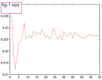
Using that code, for the case n=3we can compare Monte Carlo sim-ulation to the prices in (Johnson 1987); see for example Figure 1.
6.1 Maximum Payoffs
We will first price the derivative that has payoff max(S1,S2, . . . ,Sn), where the Sisatisfy the usual properties. In fact, this is notationally quite cumbersome, and all the ideas are encapsulated in any reasonably small value of n, so we choose n=4(as we will see later, the fourth asset will be the strike).
Firstly, the value of the derivative is the sum of the value of 4 other derivatives, the ithof which pays Si(T)if Si(T) >Sj(T)for j=i, and 0
other-wise. Let us value the first of these, the others will have similar values just by cycling the coefficients.
We are considering the asset that pays S1(T) if S1(T) is the largest price. Now let S1 be the numeraire asset with associated martingale
measure Q1. We see that the value of the derivative is
V1(t)=S1(t)e−q1τEQ1 t [1;S2/1(T) <1, S3/1(T) <1, S4/1(T) <1] =S1(t)e−q1τQ 1[S2/1(T) <1, S3/1(T) <1, S4/1(T) <1] =S1(t)e−q1τQ 1[lnS2/1(T) <0, lnS3/1(T) <0, lnS4/1(T) <0] (6) where Si/j(T)=SSi(T) j(T).
Let σi/j= ai−aj. We know that under Qjwe have dSi/j
Si/j =(qj−qi)dt+
(ai−aj)·dW
j, so lnSi
/j(T)∼φ(lnSi/j(t)+(qj−qi−12σi/2j)τ , σi/j√τ).
Note that, and define
σi2/j=σ 2 i +σ 2 j −2ρijσiσj di±/j= lnSi(t) Sj(t) + qj−qi±1 2σ 2 i/j (τ ) σi/j√τ di±= lnSi(t) K + r−qi±1 2σ 2 i (τ ) σi√τ Hence Qj[Si/j(T) <>1]=N(∓d i/j −). Note that di±/j= −dj∓/i.
Also, the correlation between Si/k(T)and Sj/k(T)is
ρij,k:= (ai−ak)·(aj−ak) ai−akaj−ak = ai·aj−ai·ak−ak·aj+σ 2 k (σ2 i +σ 2 k −2ai·ak)(σ 2 j +σ 2 k −2aj·ak) = ρijσiσj−ρikσiσk−ρkjσkσj+σk2 (σ2 i +σ 2 k −2ρikσiσk)(σ 2 j +σ 2 k −2ρjkσjσk) (7) Hence Q1[lnS2/1(T) <0, lnS3/1(T) <0, lnS4/1(T) <0]=N3(−d 2/1 − ,−d3−/1
,-d4−/1,1)where 1, 2, 3and 4are 3×3matrices; the simplest way to think of them is that they are initially 4×4matrices, with khaving ρij,k
in the (i,j)th position, and then the kthrow and kthcolumn are removed.
Thus, the value of the derivative that pays off the largest asset is
Vmax(t)=S1(t)e−q1τN3(−d 2/1 − ,−d3−/1,−d4−/1, 1) +S2(t)e−q2τN3(−d1/2 − ,−d3−/2,−d4−/2, 2) +S3(t)e−q3τN3(−d1/3 − ,−d2−/3,−d4−/3, 3) +S4(t)e−q4τN3(−d1/4 − ,−d2−/4,−d3−/4, 4) =S1(t)e−q1τN3(−d2/1 − ,−d3−/1,−d−4/1, ρ23,1, ρ24,1, ρ34,1) +S2(t)e−q2τN3(−d1/2 − ,−d3−/2,−d−4/2, ρ13,2, ρ14,2, ρ34,2) +S3(t)e−q3τN3(−d1/3 − ,−d2−/3,−d−4/3, ρ12,3, ρ14,3, ρ24,3) +S4(t)e−q4τN3(−d1/4 − ,−d2−/4,−d−3/4, ρ12,4, ρ13,4, ρ23,4) (8)
6.2 Best and Worst of Call Options
Let us start with the case where the payoff is the best of assets or cash. The payoff at expiry is max(S1, S2, S3, K). If we consider this to be the best of four assets, where the fourth asset satisfies S4(t)=Ke−rτ and has
zero volatility, then we recover the value of this option from §6.1. This fourth asset not only has no volatility but also is independent of the other three assets.
Thus, a4=0,ρij,4=ρij, σi/4=σi=σ4/i, d i/4 ± =di±, d4±/i= −di∓. Thus
^
TECHNICAL ARTICLE
3
0 5 10 15 20 25 30 35 40 45 50 6.21 6.215 6.22 6.225 6.23 6.235 6.24Figure 1: Monte Carlo for call on minimum on 3 assets. On the hori-zontal axis: number of experiments in 1000’s, using independent Sobol sequences, on the vertical axis: price. The exact option value using the formula presented here is 6.2273.
+Ke−rτN3(−d1
−,−d2−,−d3−, ρ12, ρ13, ρ23) Now let us consider the rainbow call on the max option.
Recall, this has payoff max(max(S1,S2,S3)−K,0). Note that max(max(S1,S2,S3)−K,0)=max(max(S1,S2,S3),K)−K
=max(S1,S2,S3,K)−K and so Vcmax(t)=S1(t)e−q1τN3(−d 2/1 − ,−d3−/1,d1+, ρ23,1, ρ24,1, ρ34,1) +S2(t)e−q2τN3(−d1/2 − ,−d3−/2,d2+, ρ13,2, ρ14,2, ρ34,2) +S3(t)e−q3τN3(−d1/3 − ,−d2−/3,d3+, ρ12,3, ρ14,3, ρ24,3) −Ke−rτ[1−N 3(−d1 −,−d2−,−d3−, ρ12, ρ13, ρ23)] (10)
Finally, we have the rainbow call on the min option. (Recall, this has payoff max(min(S1,S2,S3)−K,0).) Because of the presence of both a maximum and minimum function, new ideas are needed. As before we first value the derivative whose payoff is max(min(S1,S2,S3),S4).
If S4is the worst performing asset, then the payoff is the second worst
performing asset. For 1≤i≤3the value of this payoff can be found by using asset Si as the numeraire. For example, the value of the derivative that pays S1, if S4is the worst and S1the second worst performing asset, is
S1(t)e−q1τN3(d2/1
− ,d3−/1,−d−4/1, ρ23,1,−ρ24,1,−ρ34,1)
If S4is not the worst performing asset, then the payoff is S4. Now the
probability that S4is the worst performing asset is
N3(d1−/4,d2−/4,d3−/4, ρ12,4, ρ13,4, ρ23,4)
and so the value of the derivative that pays S4, if S4 is not the worst
per-forming asset, is
S4(t)e−q4τ[1−N3(d1/4
− ,d2−/4,d−3/4, ρ12,4, ρ13,4, ρ23,4)]
Thus, the value of the derivative whose payoff is max(min(S1,S2,
S3),S4)is V(t)=S1(t)e−q1τN3(d2/1 − ,d3−/1,−d−4/1, ρ23,1,−ρ24,1,−ρ34,1) +S2(t)e−q2τN3(d1/2 − ,d3−/2,−d−4/2, ρ13,2,−ρ14,2,−ρ34,2) +S3(t)e−q3τN3(d1/3 − ,d2−/3,−d−4/3, ρ12,3,−ρ14,3,−ρ24,3) +S4(t)e−q4τ[1−N3(d1/4 − ,d2−/4,d−3/4, ρ12,4, ρ13,4, ρ23,4)] (11)
Hence the derivative with payoff max(min(S1,S2,S3),K)has value
V(t)=S1(t)e−q1τN3(d2/1 − ,d3−/1,d1+, ρ23,1,−ρ24,1,−ρ34,1) +S2(t)e−q2τN3(d1/2 − ,d3−/2,d2+, ρ13,2,−ρ14,2,−ρ34,2) +S3(t)e−q3τN3(d1/3 − ,d2−/3,d3+, ρ12,3,−ρ14,3,−ρ24,3) +Ke−rτ[1−N 3(d1 −,d2−,d3−, ρ12, ρ13, ρ23)] (12) −Ke−rτN3(d1 −,d2−,d3−, ρ12, ρ13, ρ23)
7. Finding the Value of Puts
This is easy, because put-call parity takes on a particularly useful role. It is always the case that
Vc(K)+Ke−rτ =Vp(K)+Vc(0) (14)
where the parentheses denotes strike. Vcould be an option on the mini-mum, the maximini-mum, or indeed any ordinal of the basket. If we have a formula for Vc(K), as established in one of the previous sections, then we can evaluate Vc(0)by taking a limit as K ↓0, either formally (using facts of the manner N2(x,∞, ρ)=N1(x) and N3(x,y,∞, )=N2(x,y, ρxy)) or
informally (by forcing our code to execute with a value of K which is very close to, but not equal to, 0 - thus avoiding division by 0 problems but implicitly implementing the above-mentioned fact). By rearranging, we have the put value.
8. Deltas of Rainbow Options
By inspecting (9) one might expect that∂Vmax ∂S1
=e−q1τN3(−d2/1
− ,−d3−/1,d1+, ρ23,1, ρ24,1, ρ34,1)
with similar results holding for ∂Vmax
∂S2 and
∂Vmax
∂S3 , and indeed for the dual
delta ∂Vmax
∂K .
Thus turns out to be true in this case, but to claim it as an ‘obvious fact’ would be erroneous. Recall Euler’s Homogeneous Function Theorem, which we will cast in our case of a function of four variables V(x1,x2,x3,x4). The theorem states that if V(λx1, λx2, λx3, λx4)=λV(x1,x2,x3,x4)for any
constant λthen V(x1,x2,x3,x4)=x1∂∂xV 1 +x2 ∂V ∂x2 +x3 ∂V ∂x3 +x4 ∂V ∂x4.
The argument of (Johnson 1987) is essentially an application of this theorem: he intuits what ∂V
∂Si is and then ‘reassembles’ Vusing this result.
However, to claim a converse of the form that if V(x1,x2,x3,x4)=
x11+x22+x33+x44 for some ‘nice’ ithen of necessity i=∂∂xV
i
is false. (6) provides a counterexample; because certainly it is not the case that ∂V
∂Si =0for i>1. To jump at the claim that it is an obvious fact that
the above is the formula for delta is probably an application of this false converse.
However, these claims are true in the case of Vmax, as it is for Vcmax,
Vcmin, Vpmax and Vpmin.
9 Finding the Capital Guarantee on the
‘Best of Assets or Cash Option’
value of such an option as V(K)—implicitly fixing all other variables be-sides the strike—we wish to solve V(K)=K.
To do so using Newton’s method is fortunately quite manageable, for the same reasoning that we have already seen. As previously promised we have from (9) that
∂V
∂K =e
−rτ
N3(−d1−,−d2−,−d3−, ρ12, ρ13, ρ23)
Hence the appropriate Newton method iteration is
Kn+1=Kn−
V(Kn)−Kn
∂V
∂K|K=Kn−1
(15)
and this is iterated to some desired level of accuracy. An alternative would be to iterate Kn+1=V(Kn), our differentiation shows that the
func-tion V is a contraction, and so this iteration will converge to the fixed point V(K)=Kby the contraction mapping theorem.
It is important to note that the process of finding the fair theoretical strike is not just a curiosity. In the first place, it is attractive for the buyer of the option that they will get at least their premium back. (There is a floor on the return of 0%.) Moreover, if Kis this fair strike, the trader will strike the option at an K∗, where K∗>K, in order to expect fat in the deal. To see this, we can construct in a complete market a simple arbitrage strategy: imagine that the dealer sells the client for K∗an option struck at
K∗, and hedges this with the ‘fair’ dealer by paying Kfor an option struck at K.1The difference K∗−K is invested in a risk free account for the ex-piry date. Three cases then arise:
• If max(S1,S2,S3)≤K then we owe K∗. The fair trader pays K and we obtain K∗−Kfrom saving, and profit from the time value of K∗−K. • If K<max(S1,S2,S3)≤K∗, then the fair trader pays S1 say. We sell
this, and obtain the balance to K∗from saving.
• If K∗<max(S1,S2,S3), then the fair trader pays S1say and we deliver
this.
10 Pricing Rainbow Options in Reality
The model that has been developed here lies within the classical Black-Scholes framework. As is well known, the assumptions of that framework do not hold in reality; various stylised facts argue against that model. For vanilla options, the model is adjusted by means of the skew—this skew ex-actly ensures that the price of the option in the market is exex-actly cap-tured by the model. Models which extract information from that skew and of how that skew will evolve are of paramount importance in mod-ern mathematical finance.After a moment’s thought one will realise what a difficult task we are faced with in applying these skews here. Let us start by being completely naïve: we wish to mark our rainbow option to market by using the skews of the various underlyings. Firstly, what strike do we use for the underly-ing? How does the strike of the rainbow translate into an appropriate strike for an option on a single underlying? Secondly, suppose we some-how resolved this problem, and for a traded option, wished to know its implied volatility? A familiar problem arises: often the option will have
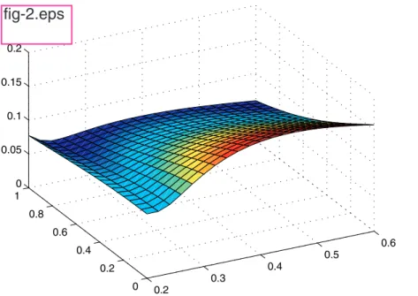
two, sometimes even three different volatilities of one of the assets which recover the price (all other inputs being fixed). To be more mathematical, the map from volatility to price is not injective, so the concept of implied volatility is ill defined. See Figure 2.
To see the sensitivity to the inputs, suppose to the setup in Figure 2 we add a third asset as elaborated in Figure 3. Of course the general level
^
TECHNICAL ARTICLE
3
0.2 0.3 0.4 0.5 0.6 0 0.2 0.4 0.6 0.8 1 0 0.05 0.1 0.15 0.2Figure 2: The price for a call on the minimum of two assets. S1= 2, S2= 1, K= 1,
τ= 1, r= 10%, ρ= –70%, 20% ≤ σ1≤60%, σ2 ≤100%. 00.2 0.3 0.4 0.5 0.6 0.2 0.4 0.6 0.8 1 0 0.01 0.02 0.03 0.04 0.05
Figure 3: The price for a call on the minimum of three assets. As above, in addition S3= 1, σ3 = 30% fixed, correlation structure ρ12 = –70%, ρ13 =
30%, ρ23 = –20%.
fig-2.eps
W
of the value of the asset changes, but so does the entire geometry of the price surface.
Another issue is that of the assumed correlation structure: again, cor-relation is difficult to measure; if there is implied data, then it will have a strike attached. Finally, the joint normality hypothesis of returns of prices will typically be rejected.
A popular approach is to use skews from the vanilla market to infer the marginal distribution of returns for each of the individual assets and then ‘glue them together’ by means of a copula function. Given a multi-variate distribution of returns, rainbow options can then be priced by Monte Carlo methods.
■Genz, A. (2004) ‘Numerical computation of rectangular bivariate and trivariate normal
and t probabilities’, Statistics and Computing14, 151–160.
*http://www.sci.wsu.edu/math/faculty/genz/homepage
■Harrison, J. M. & Pliska, S. R. (1981), ‘Martingales and stochastic integrals in the theory
of continuous trading’, Stochastic Processes and their Application11, 215–260.
■Johnson, H. (1987) ‘Options on the maximum or the minimum of several assets’,
Journal of Financial and Quantitative Analysis22, 277–283.
■Margrabe, W. (1978), ‘The value of an option to exchange one asset for another’, The
Journal of Finance23, 177–186.
■Rubinstein, M. (1991) ‘Somewhere over the rainbow’, Risk4, 63–66.
■Stulz, R. M. (1982), ‘Options on the minimum or the maximum of two risky assets’,
Journal of Financial Economics XXXIII, No. 1, 161–185.
■West, G. (2005), ‘Better approximations to cumulative normal functions’, WILMOTT
MagazineMay, 70–76.
ACKNOWLEDGEMENTS
Thanks to the 2005 Mathematics of Finance class at the University of the Witwatersrand for alert feedback in lectures.
1.The ‘fair’ dealer is the perfect hedger, whose replicating portfolio ends up with
exactly the payoff.
■Geman, H., El Karoui, N. & Rochet, J. (1995) ‘Changes of numeraire, changes of
prob-ability measure and option pricing’, Journal of Applied Probability32.