Central Washington University Central Washington University
ScholarWorks@CWU
ScholarWorks@CWU
All Faculty Scholarship for the College of the
Sciences College of the Sciences
2-3-2014
Visualization of multidimensional data with collocated paired
Visualization of multidimensional data with collocated paired
coordinates and general line coordinates
coordinates and general line coordinates
Boris KovalerchukFollow this and additional works at: https://digitalcommons.cwu.edu/cotsfac
Kovalerchuk, B., Visualization of multidimensional data with collocated paired coordinates and general line coordinates,
In: SPIE Visualization and Data Analysis 2014, Proc. SPIE 9017, Paper 90170I, doi: 10.1117/12.2042427, 15 p.
Visualization of multidimensional data with collocated paired
coordinates and general line coordinates
Boris Kovalerchuk*
Dept. of Computer Science, Central Washington University, USA
ABSTRACT
Often multidimensional data are visualized by splitting n-D data to a set of low dimensional data. While it is useful it destroys integrity of n-D data, and leads to a shallow understanding complex n-D data. To mitigate this challenge a difficult perceptual task of assembling low-dimensional visualized pieces to the whole n-D vectors must be solved. Another way is a lossy dimension reduction by mapping n-D vectors to 2-D vectors (e.g., Principal Component Analysis). Such 2-D vectors carry only a part of information from n-D vectors, without a way to restore n-D vectors exactly from it. An alternative way for deeper understanding of n-D data is visual representations in 2-D that fully preserve n-D data. Methods of Parallel and Radial coordinates are such methods. Developing new methods that preserve dimensions is a long standing and challenging task that we address by proposing Paired Coordinates that is a new type of n-D data visual representation and by generalizing Parallel and Radial coordinates as a General Line coordinates. The important novelty of the concept of the Paired Coordinates is that it uses a single 2-D plot to represent n-D data as an oriented graph based on the idea of collocation of pairs of attributes. The advantage of the General Line Coordinates and Paired Coordinates is in providing a common framework that includes Parallel and Radial coordinates and generating a large number of new visual representations of multidimensional data without lossy dimension reduction.
Keywords: Multivariate data, visualization ,multidimensional data ,collocated paired coordinates, parallel coordinates,
general line coordinates, radial coordinates, axis reconfiguration.
1. INTRODUCTION
The Big Data studies revealed that now every few days more data are created than for all previous centuries. This leads
to tremendous challenges to process and manage these data. Visual analytics is a promising approach to deal with this challenge. Information management and decision making can benefit significantly from visualization and visual analytics that support multiple coordinated visual representations of multivariate and multilevel data to understand these data. Splitting multidimensional n-D data to a set of low dimensional data destroys integrity of n-D data, and leads only to a shallow understanding such complex n-D data. This paper attempts to address this long standing and challenging task20, 48 by generalizing Parallel and Radial coordinates and by proposing Paired Coordinates that is a new type of n-D data visual representation.
We formulate a common main idea behind Parallel, Radial and Paired Coordinates as a tradeoff a simple n-D point that
has no internal structure for a 2-D line that has the internal structure. In short here the dimensionally is traded for a
structure. Every object with an internal structure includes two or more points. The only elements in 2-D that do not
overlap if they are not equal are 2-D points. Other unequal 2-D objects that contain more than one point can overlap. Thus, clutter is a direct result of this tradeoff. The only way fundamentally to avoid clutter is locating structured 2-D objects side-by-side as it is done with Chernoff faces. The price for this is more difficulty in correlating features of the faces relative to objects that are stacked38.
A multivariate dataset consists of n-tuples (n-D vectors), where each element of an n-D vector is a nominal or ordinal
value corresponding to an independent or dependent variable. The techniques to display multivariate data are classified in17 as:
(1) Axis reconfiguration techniques, such as parallel coordinates22,23,46 and radial/star coordinates14,
(2) Glyphs2,8,27, 37,
(3) Dimensional embedding techniques, such as dimensional stacking31 and worlds within worlds15,
(4) Dimensional subsetting, such as scatterplots10,
(5) Dimensional reduction techniques, such as multidimensional scaling30,32, 47, principal component analysis24 and
self-organizing maps26.
Axis reconfiguration and Glyphs map axis into another coordinate system. Chernoff faces map axis onto facial features
(icons). Glyphs /Icons are a form of multivariate visualization in orthogonal 2-D coordinates that augment each spatial point with a vector of values, in the form of a visual icon that encodes the values coordinates35. The glyph approach is more limited in dimensionality than parallel coordinates17. There is also a type of glyph visualization where each number in the n-D vector is visualized individually. For instance, a vector (0, 0.25, 0.5, 0.75, 1) is represented by a sting of Harvey balls or by color intensities. This visualization is not scaled well for large number of vectors and large dimensions, but it is interesting conceptually because it is does not use lines to connect values in the visualization. These lines are a major source of the clutter in visualizations based on Parallel and Radial coordinates. Parallel coordinates and radial coordinates are a planar representation of an n-D space that map points to polylines. The transformation to the planar representation means that axis reconfiguration and glyphs trade a structurally simple n-D object to a more complex object, but in a lower dimension (complex 2-D face, or polyline vs. a simple n-D list of numbers). Pixel oriented techniques map n-D points to a pixel-based area of some properties such as color or shape25, 16.
Dimensional subsetting literally means that a set of dimensions (attributes) splat/sliced into subsets, e.g., pairs of
attributes (Xi,Xj) and each pair is visualized by a scatterplot with total n2 of scatterplots that for a matrix of scatterplots.
Dimensional embedding also is based on subsets of dimensions, but with specific roles. The dimensions are divided into
those that are in the slice and those that create the wrapping space where these slices are then embedded at their respective position36.
Technically (1)-(4) are lossless transformations, but the dimensional reduction is not. Among lossless representations only (1) and (2) preserve n-D integrityof data. In contrast (3) and (4) split each n-D record adding a new perceptual task of assembling low-dimensional visualized pieces of each record to the whole record. Therefore, we are interested in enhancing (1) and (2).
The examples of (1) and (2) listed above fundamentally try to represent visually actual values of all attributes of an n-D point. This ensures lossless representation, but is fundamentally limiting the size of the dataset that can be visualized17. The good news is that visualizing all attributesis not necessary for lossless representation. The position of the visual element on 2-D plane can be sufficient to restore completely the n-D vector as it was shown for Boolean vectors in27-29.
This paper is organized as follows. Section 2 presents the General Line coordinates that generalizethe Parallel and Radial Coordinates that are well known lossless methods to visualize n-D data in 2-D that do not require data splitting. Section 3 presents a class of Paired Coordinates that is a new class of lossless n-D data visualizations that are also free from data splitting. Section 4 compares the Paired Coordinates with other methods. The benefits of the Paired Coordinates are illustrated with examples that include World hunger data and Challenger Space Shuttle disaster. Section 5 summarizes this paper.
2. GENERAL LINE COORDINATES AS GENERALIZATION OF PARALLEL AND RADIAL
COORDINATES
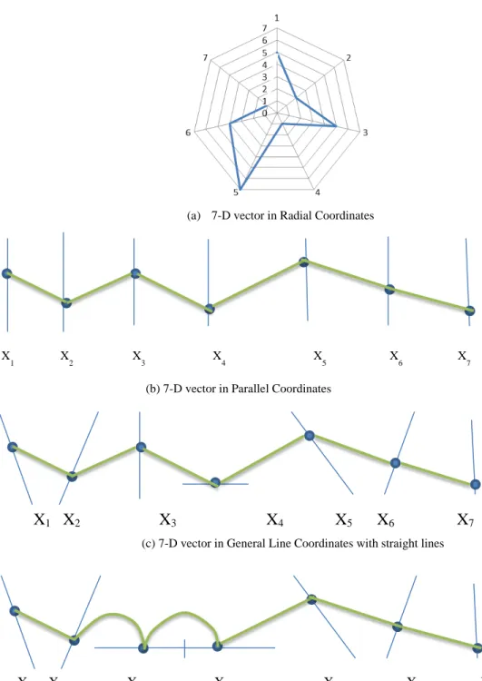
In a traditional Radial Coordinates also known as a star plot the axes for variables radiate in equal angles from a common origin. A line segment is drawn along each axis starting from the origin and the length of the line representing the value of the related variable (Figure 1a). Often the tips of the star's beams are connected in order to create a closed star shape1,38. A closed contour is not required to have a full representation of the n-D vector. For instance, a link between xn and x1 can be skipped.
Without closing the line radial and parallel coordinates (Figure 1b) are mathematically equivalent /homomorphic. For every point p on radial coordinate X a point q exists in the parallel coordinate X that has the same value as p. The difference is in the geometric layout (radial or parallel) of n-D coordinates on the 2D plane. The next difference is that sometimes in the Radial Coordinates each n-D vector is shown as a separate small plot that serves as an icon of that n-D vector. In the parallel coordinates all n-D vectors are shown on the same plot. To make the use of the radial coordinates less occluded at the area close to the common origin of the axis a non-linear scale can be used to spread data that are close to the origin. Figure 1 shows Radial, Parallel and Generalized coordinates called General Line Coordinates
(GLC). These GLC coordinates can go in any direction, be of different length, be connected or disconnected, and use curvilinear lines.
Figure 1. General line coordinates with arbitrary directions of line coordinates X1,X2,…X7.
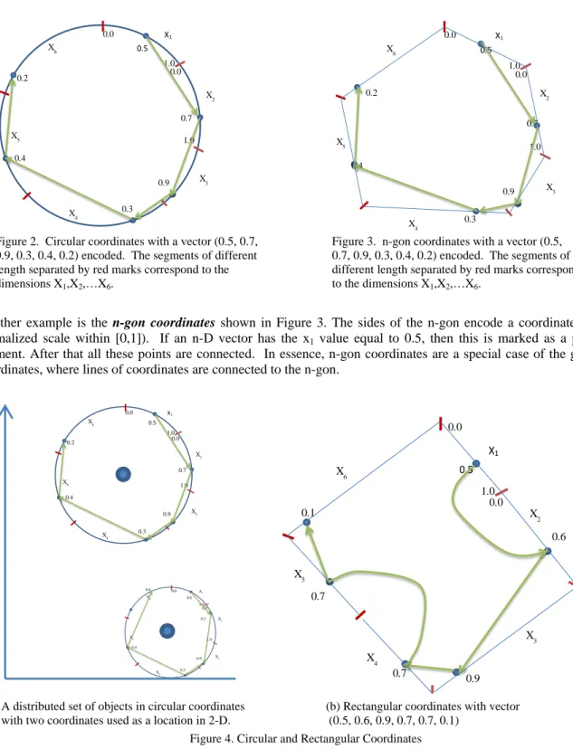
Figure 2 shows a form of the GLC where coordinates are connected to form a circle. We call it Circular Coordinates. The circle is splat to segments and each segment encodes a coordinate (e.g., in a normalized scale within [0,1]). If an n-D vector has x1 value equal to 0.5 then this is marked as a point on x1 segment. Then all these points are connected to form an oriented graph.
X
1X
2X
3X
4X
5X
6X
7X1 X2 X3 X4 X5 X6 X7 X
1 X2 X3 X4 X5 X6 X7 (b) 7-D vector in Parallel Coordinates
(c) 7-D vector in General Line Coordinates with straight lines
(d) 7-F vector in General Line Coordinates with curvilinear lines (a) 7-D vector in Radial Coordinates
Figure 2. Circular coordinates with a vector (0.5, 0.7, 0.9, 0.3, 0.4, 0.2) encoded. The segments of different length separated by red marks correspond to the dimensions X1,X2,…X6.
Figure 3. n-gon coordinates with a vector (0.5, 0.7, 0.9, 0.3, 0.4, 0.2) encoded. The segments of different length separated by red marks correspond to the dimensions X1,X2,…X6.
Another example is the n-gon coordinates shown in Figure 3. The sides of the n-gon encode a coordinate (e.g., in a normalized scale within [0,1]). If an n-D vector has the x1 value equal to 0.5, then this is marked as a point on x1 segment. After that all these points are connected. In essence, n-gon coordinates are a special case of the general line coordinates, where lines of coordinates are connected to the n-gon.
(a) A distributed set of objects in circular coordinates with two coordinates used as a location in 2-D.
(b) Rectangular coordinates with vector (0.5, 0.6, 0.9, 0.7, 0.7, 0.1)
Figure 4. Circular and Rectangular Coordinates
Circular and n-gone coordinates also can be used with splitting coordinates where two coordinates are used to identify location of the center and n-2 coordinates are used build a circle or (n-2)-gon at that location with appropriate scaling these n-gons will not overlap (Figure 4a). This is a way to represent geospatial data and a link to the glyph-based visualization of n-D data. The lines of coordinates in the generalized coordinates can also continue straight each other
without any turn between them as shown in Figure 4b. For instance, if n-gon is a rectangle or a square then each edge of the square can split to sections that will represent several dimensions as shown in Figure 4b.
X1 X2 X3 X4 X5 X6 0.5 0.7 0.9 1.0 0.0 0.0 1.0 0.3 0.4 0.2 X1 X 2 X 3 X 4 X 5 X 6 0.5 0.7 0.9 1.0 0.0 0.0 1.0 0.3 0.4 0.2 X1 X2 X3 X4 X 5 X 6 0.5 0.7 0.9 1.0 0.0 0.0 1.0 0.3 0.4 0.2 X1 X2 X3 X4 X5 X6 0.5 0.2 0.9 1.0 0.0 0.0 1.0 0.3 0.4 0.6 X1 X2 X3 X 4 X5 X6 0.5 0.6 0.9 1.0 0.0 0.0 0.7 0.7 0.1
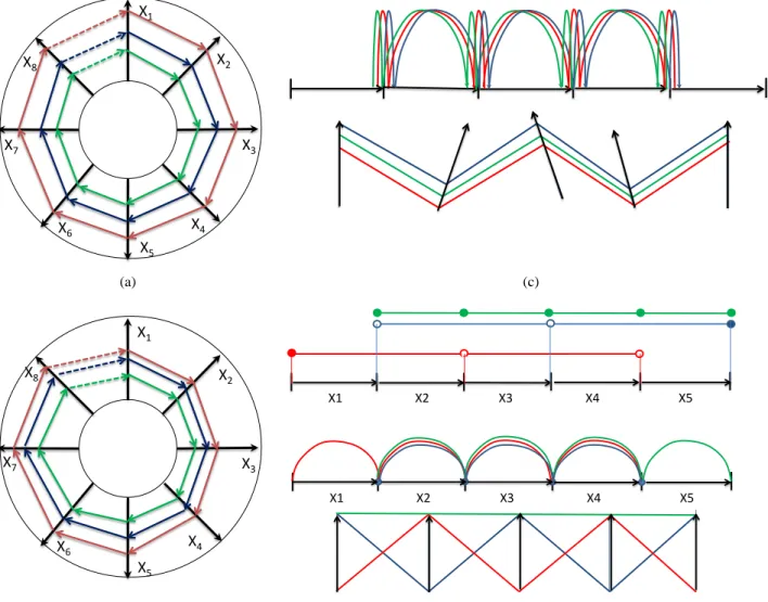
The parallel and radial coordinates have an good visual property: lines for two n-D vectors do not cross each other if these vectors are ordered, e.g., vector x1 =(x11,x12,…,x1n) is greater or equal to vector x2 =(x21,x22,…,x2n) if for every i=1,…,n x1i ≥x2i. Figure 5 illustrate this and other properties for several vectors:
(a) x1=(0.8,0.8,0.8,0.8,0.8,0.8,0.8,0.8) (magenta); x2=(0.6,0.6,0.6,0.6,0.6,0.6,0.6,0.6) (blue), and x3=(0.4,0.4,0.4,0.4,0.4, 0.4,0.4,0.4) (green).
(b) x1=(0.6,0.6,0.6,0.6,0.7 0.8,0.8,0.8) (magenta); x2=(0.5,0.5,0.5,0.5,0.5,0.6,0.6,0.6) (blue), and x3=(0.4,0.3,0.3,0.3,0.3, 0.5,0.5,0.5) (green).
(c) x1=(1.0,0.2,1.0,0.2,1.0) (blue); x2=(0.9,0.1,0.9,0.1,0.9) (red); x3=(0.8,0.0, 0.8, 0.0,0.8) (green). (d) x1=(1,0,1,0,1) (blue); x2=(0,1,0,1,0) (red); x3=(1,1,1,1,1) (green).
(a) (c)
(b) (d)
Figure 5. Visual patterns in general line coordinates
Traditional radial coordinates have a difficulty to display data that are close to the origin of the coordinates. These data occlude each other because the area next to the common origin is too small. The general line coordinates shown on Figure 5a and Figure 5b resolve this issue. This is a modified radial coordinates where coordinates have no common origin. This is one of the advantages of a large class of general line coordinates visualizations. In Figure 5a each n-D vector (with all equal values of coordinates) is represented by some n-gon. In Figure 5b the n-gon pattern is still visible while values of all coordinates of each n-D vectors are not equal.
X1 X2 X3 X4 X5 X6 X7 X8 X1 X2 X3 X4 X5 X6 X7 X8 X1 X2 X3 X4 X5 X1 X2 X3 X4 X5 c
A set of correlated vectors forms another visual pattern that is a set of nested gons (Fgure 5a) and a set of distorted n-gons (Figure 5b). In parallel and non-vertical (“inclined”) coordinates (second plot in Figure 5c) this pattern is a set of parallel polylines. In a “horizontal” coordinates (first plot in Figure 5c) this visual pattern is very distinct too.
Figure 5d illustrates visualization of three n-D vectors in different general line coordinates when vectors are not correlated. While each n-D vector has a distinct visual pattern itself the set of three n-D vectors does not form a common visual pattern, which is expected for uncorrelated vectors. The top plot in Figure 5d shows these vectors in the “horizontal” coordinates when oriented graphs are simplified to decrease clutter (vertical lines are omitted for the green line and deemphasized for the red and blue lines). It shows that patterns for these vectors are quite different. The next visualizations in Figure 5 also show difference in visual patterns in their own ways.
The ultimate benefit from different general line coordinates would be discovering visual patterns within individual n-D vectors and within a set of n-D vectors and converting these visual patterns to analytical mathematical forms. It is appropriate to do this in two separate steps: (1) getting distinct visual patterns for different subsets of the dataset by finding an appropriate GLC, and (2) finding analytical mathematical properties that would describe these visual patterns. For instance, the middle plot in Figure 5d shows visually a repetition pattern of half-circles more clearly than other GLC visualizations of the same data in Figure 5d. Thus half-circles serve as a good clue for discovering a mathematical rule for the pattern. Only for very simple patterns this can be done in one step where the math properties are observed directly from the visual patterns. For the complex ones this cannot be expected and rather a complex analysis is required to transform a discovered visual pattern to a mathematical form.
The second plot in Figure 5c shows three correlated 5-D vectors in the “inclined” GLC that are not parallel. These coordinates keep familiar visual pattern of correlated vectors presented in the parallel coordinates. What could be an advantage of such coordinates relative to the parallel coordinates? If data are correlated in two coordinates then these coordinates can be shown in GLC inclined to each other if the correlation is positive (coordinates arrows have the same direction). This can be a clue to analyze the correlation plot for these coordinates. Moreover the correlation plot can be overlaid with these two coordinates in GLC. It would require locating these coordinates orthogonally in the GLC.9
3. PAIRED COORDINATES
3.1 Definitions
The idea of the paired coordinates is converting a simple string of elements of vector x=(x1,x2,…xn) in coordinates X1, X2, …, Xn to a more complex structure with consecutive 2-D elements (pairs) for even n:
{(x1,x2) (x3,x4),…,(xi,xi+1) , …,(xn-3,xn-2), (xn-1,xn)}. .
These pairs have no common elements. For the odd n this structure is slightly different:
{(x1,x2) (x3,x4),…,(xi,xi+1) , …,(xn-2,xn-1), (xn-1,xn-)}
that is with pairs (xn-2,xn-1) and (xn-1,xn) where xn-1 is common to both pairs. Without such overlap the last element xn will not have a pair. Alternatively, xn can form a pair with itself for an odd n:
{(x1,x2) (x3,x4),…,(xi,xi+1) , …,(xn-2,xn-1), (xn,xn)}.
The scales of coordinates X1-Xn are normalized to some interval, e.g., [0,1] and constructed pairs (xi,xi+1) are plotted on the same (X,Y) 2-D plane. The example below illustrates this process.
Consider six variables, a state vector x=(x, y, x`, y`, x``, y``) in these coordinates, where x and y are location coordinates of the object, x` and y` are velocities (derivatives), and x`` and y`` are accelerations (second derivatives) of this object. The algorithm to represent vector x in collocated paired coordinates is as follows:
Step 1. Normalizing each coordinate to some interval, e.g., the interval [0,1]. Step 2. Grouping elements of x as consecutive pairs (x,y) (x`,y`) (x``,y``). Step 3. Plotting orthogonal normalized Cartesian coordinates X and Y.
Step 4. Plotting point (x,y) on (X,Y) Step 5. Plotting point (x`,y`) on (X,Y) Step 6. Plotting point (x``,y``) on (X,Y).
Step 7. Plotting a directed graph (x,y) →(x`,y`) → (x``,y``) with directed paths from (x,y) to (x`,y`) and from (x`,y`) to (x``,y``).
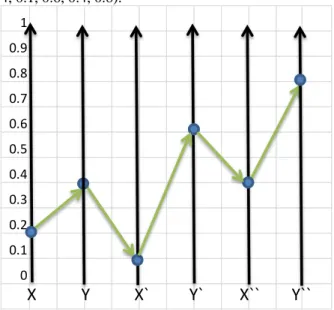
An example is shown in Figure 6 for x=(x,y,x`,y`,x``,y``)=(0.2, 0.4, 0.1, 0.6, 0.4, 0.8).
(a) Collocated Paired coordinates (b) Parallel coordinates Figure 6. Vector x=(x,y,x’,y’,x’’,y’’)=(0.2,0.4, 0.1, 0.6, 0.4, 0.8) in paired and parallel coordinates.
(a) Radial (Anchored) paired coordinates. (b) Shifted paired coordinates Figure 7. Radial and Shifted paired coordinates with vector x=(x,y,x’,y’,x’’,y’’)=(0.2 ,0.4, 0.1, 0.6, 0.4, 0.8)
Figure 7 shows an alternative version of the paired coordinates --radial paired coordinates, where (x`,y`) and (x``,y``) are considered as a vector that start at point (x,y) as an anchor. At the formal level it means that we plot two vectors
((x,y), (x+x`,x+y`)), ((x,y), (x+x``,x+y``)) or ((x,y), (x+x`,x+y`)), ((x+x`,x+y`), (x+x``,x+y``)).
1 0.9 0.8 0.7 0.6 0.5 0.4 0.3 0.2 0.1 0 0 0.1 0.2 0.3 0.4 0.5 0.6 0.7 0.8 0.9 1 (0.2, 0.4)=(x,y) (0.1, 0.6)=(x`,y`) (0.4, 0.8)=(x``,y``) 1 0.9 0.8 0.7 0.6 0.5 0.4 0.3 0.2 0.1 0
X Y X` Y` X`` Y``
1.2 0.8 1.1 0.7 1 0.6 0.9 0.5 0.8 0.4 0.7 0.3 0.6 0.2 0.5 0.1 0.4 0 0.3 0.1 0.2 0.3 0.4 0.5 0.6 0.2 0.1 0 0 0.1 0.2 0.3 0.4 0.5 0.6 0.7 0.8 0.9 1 (0.1, 0.6)+(0.2,0.4)=(0.3,1.0) (x`,y`)=(0.3,1.0)in (Xp1,Yp1) (x`,y`)=(0.1,0.6) in (Xp2,Yp2) (Xp1,Yp1) (0.4, 0.8)+(0.2,0.4)=(0.6,1.2) (x``,y``)=(0.6,1.2) in (Xp1,Yp1) (x``,y``)=(0.4,0.8) in (Xp1,Yp2) (x,y)=(0.2,0.4) in (Xp1,Yp1) (x,y)=(0,0) in (Xp2,Yp2) 1 2 (Xp2,Yp2) 1 0.8 0.9 0.7 0.8 0.6 0.7 0.5 0.6 0.4 0.5 0.3 0.4 0.2 0.3 0.1 0.2 0 (Xp3,Yp3) 0.1 (Xp2,Yp2) 0 0 0.1 0.2 0.3 0.4 0.5 0.6 0.7 0.8 0.9 1 (0.2, 0.4)=(x,y) in (Xp1,Yp1) (0.4, 0.8)=(x``,y``) in (Xp3,Yp3) (0.1, 0.6)=(x`,y`) in (Xp2,Yp2) (Xp1,Yp1)Visually it is similar to radial coordinates where the directions of axes are defined by the actual data. In contrast with the radial coordinates such directions can overlap. On the other side the advantage of the radial paired coordinates is that the direction has a meaning as actual vectors of velocity and acceleration in this example.
In the radial coordinated the directions are arbitrary. An example is shown in Figure 7a for the same vector as above in Figure 6, x=(x,y,x`,y`,x``,y``) = (0.2,0.4, 0.1, 0.6, 0.4, 0.8).
Steps 1-4 of the radial paired coordinates are the same as for collocated paired coordinates and steps 5-7 are as follows: Step 5. Plotting a point (x+x`,x+y`) on (X,Y) to represent (x`,y`)
Step 6. Plotting point (x+x``,y+y``) on (X,Y) to represent (x``,y``)
Step 7. Plotting a directed graph (x,y) → (x+x`,y+y`) → (x+x``,y+y``) with directed paths from (x,y) to (x+x`,y+y`) and from (x,y) to (x+x``,y+y``).
For comparison Figure 6b shows the same vector x in the parallel coordinates. It requires 5 lines to show x, in contrast both collocated and radial coordinates require only 2 lines. This leads to less clutter when multiple n-D vectors are visualized on the same (X,Y) coordinate plane. It is a general property of the paired coordinates to require two times fewer lines than the parallel coordinates require. This is an advantage of the Paired Coordinates.
Figure 7b shows another version of the paired coordinates –shiftedpaired coordinates with steps:
Step 1. Normalizing each coordinate to some interval, e.g., the interval [0,1] Step 2. Grouping elements of x as consecutive pairs (x,y) (x`,y`) (x``,y``). Step 3.
Step 3.1. Plotting orthogonal normalized Cartesian coordinates (Xp1,Yp1). Step 3.2. Setting up a shift (ax,ay).
Step 3.3. Generating a set of shifted points (0,0), (ax,ay), (2ax,2ay),…, (iax,iay) ,…,(kax,kay), where k is the number of pairs in the structure, which is the ceiling of n/2.
Step 3.4. Generating orthogonal normalized Cartesian coordinates (Xpi ,Ypi) for all k with origins in (iax,iay) with i=1,2,…, k, that is by shifting coordinates (Xp1,Yp1). In general (Xpi ,Ypi) can also be rotated relative to (Xp1,Yp1).
Step 4. Plotting point (x,y) on (Xp1,Yp1). Step 5. Plotting point (x`,y`) on (Xp2,Yp2) Step 6. Plotting point (x``,y``) on (Xp3,Yp3).
Step 7. Plotting a directed graph (x,y) →(x`,y`) → (x``,y``) with directed paths from (x,y) to (x`,y`) and from (x`,y`) to (x``,y``).
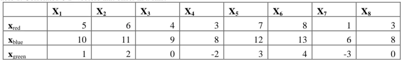
Figure 8 shows correlated data from Table 1 in the Collocated Paired Coordinates. All shapes are identical and existence of the shifts is visible. This visualization required only 3 lines for each 8-D vector instead of 7 lines in the parallel coordinates.
Table 1. Correlated 8-D vectors that differ in a shift
X1 X2 X3 X4 X5 X6 X7 X8
xred 5 6 4 3 7 8 1 3
xblue 10 11 9 8 12 13 6 8
xgreen 1 2 0 -2 3 4 -3 0
The 3-D version of Collocated Paired Coordinates is a natural generalization of the visual representations shown above by adding the Z coordinate and showing lines in 3-D.
3.2 Examples with real data
Below we provide examples of the Collocated Paired Coordinates (CPC) for two datasets: (1) World Hunger from the International Food Policy Institute [http://www.ifpri.org/book-8018/node/8058] and (2) Challenger USA Space Shuttle O-Ring Dataset relevant to Challenger disaster from the UC Irvine Machine Learning Repository4,11.12.
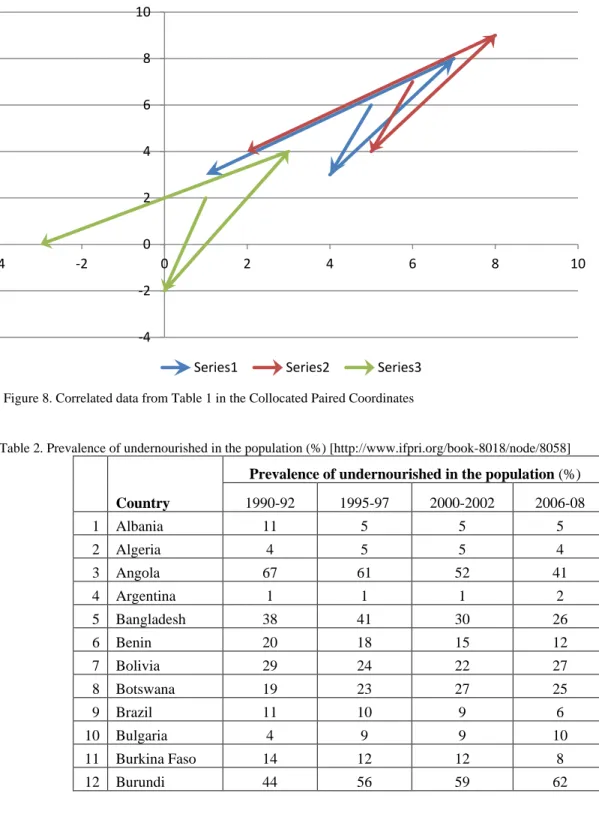
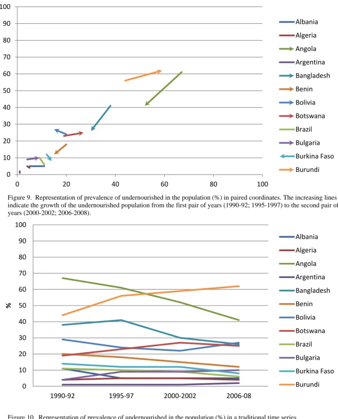
The first dataset that is a time series is shown in Table 2. Figure 9 shows these data in the Collocated Paired coordinates and Figure 10 shows them in the traditional time series. These figures show that the traditional time series required 4 lines for each 4-D vector. In contrast the CPC required only one line that do not overlap and have no any occlusion for these data again in contrast with the traditional time series.
Figure 8. Correlated data from Table 1 in the Collocated Paired Coordinates
Table 2. Prevalence of undernourished in the population (%) [http://www.ifpri.org/book-8018/node/8058]
Country
Prevalence of undernourished in the population (%)
1990-92 1995-97 2000-2002 2006-08 1 Albania 11 5 5 5 2 Algeria 4 5 5 4 3 Angola 67 61 52 41 4 Argentina 1 1 1 2 5 Bangladesh 38 41 30 26 6 Benin 20 18 15 12 7 Bolivia 29 24 22 27 8 Botswana 19 23 27 25 9 Brazil 11 10 9 6 10 Bulgaria 4 9 9 10 11 Burkina Faso 14 12 12 8 12 Burundi 44 56 59 62 -4 -2 0 2 4 6 8 10 -4 -2 0 2 4 6 8 10
Figure 9. Representation of prevalence of undernourished in the population (%) in paired coordinates. The increasing lines indicate the growth of the undernourished population from the first pair of years (1990-92; 1995-1997) to the second pair of years (2000-2002; 2006-2008).
Figure 10. Representation of prevalence of undernourished in the population (%) in a traditional time series.
The Challenger O-rings data include parameters such as (1) temporal order of flight, (2) number of O-rings at risk on a given flight, (3) number of O-rings experiencing thermal distress, (5) launch temperature (degrees F), and (5) leak-check pressure (psi). These data have been normalized to be in the [0,1] interval before visualizing them. We considered two different normalizations of the number of O-rings at risk. This number is 6 in all flights. It is normalized to 0 in the first
0 10 20 30 40 50 60 70 80 90 100 0 20 40 60 80 100 Albania Algeria Angola Argentina Bangladesh Benin Bolivia Botswana Brazil Bulgaria Burkina Faso Burundi 0 10 20 30 40 50 60 70 80 90 100 1990-92 1995-97 2000-2002 2006-08 % Albania Algeria Angola Argentina Bangladesh Benin Bolivia Botswana Brazil Bulgaria Burkina Faso Burundi
visualization and to 1 in the second visualization. The used data11 differ from data analyzed by Tufte41 (see p.44). The data used by Tufte include three erosion incidents at temperature 53F, which makes the link between low temperature and large incidents much more transparent. Draper’s data are more difficult for revealing this pattern.
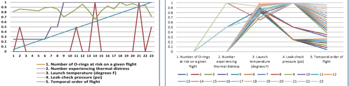
Figures 11 and 12 show visualization of Draper’s data in traditional plots. Figure 13 shows the same data in the Collocated Paired Coordinates. These figures show that the traditional time series required 4 lines for each 4-D vector. In contrast the CPC required only one line per record with low overlap and without occlusion issues for these data in contrast with the traditional time series.
Figure 11. Challenger USA Space Shuttle normalized O- Ring dataset in a traditional line chart. X coordinate is a temporal order of flights. Each line represents an attribute.
Figure 12. Challenger USA Space Shuttle normalized O-Ring dataset in a traditional line chart. X coordinate is a temporal order of flights. Each line represents a flight.
1 0.9 0.8 0.7 0.6 0.5 0.4 0.3 0.2 0.1 0 0 0.1 0.2 0.3 0.4 0.5 0.6 0.7 0.8 0.9 1 1, 3, 4,5,6 2 7 8 9,10 11 12, 16, 18, 19, 20,22 13, 15.17 14 21 23 1 0.9 0.8 0.7 0.6 0.5 0.4 0.3 0.2 0.1 0 0 0.1 0.2 0.3 0.4 0.5 0.6 0.7 0.8 0.9 1 1, 3, 4,5,6 2 7,8 9,10,23 11 12, 16, 18, 19, 20,22 13, 15.17 14 21
Figure 13. Challenger USA Space Shuttle normalized O-Ring dataset in the Collocated Paired Coordinates. X, Y coordinates are normalized values of attributes. 6 O-rings at risk are normalized as 0.
Figure 14. Challenger USA Space Shuttle normalized O-Ring dataset in the Collocated Paired Coordinates. X and Y coordinates are normalized values of attributes. 6 O-rings at risk are normalized as 1.
Figure 14 shows three distinct flights #2, #14, and #2. They have an orientation that differs from other flights. These flights had maximum value of O-rings at risk. Thus CPC visually show a distinct pattern in flights that has a meaningful interpretation. The well-known case is #14, which is the lowest temperature (53F) from the previous 23 Space Shuttle launches. It stands out in the Collocated Paired Coordinates. In the test at high leak-check pressure (200 psi) it had 2 O-rings that experienced a thermal distress. The case #2 also experienced thermal distress for one O-ring at much higher temperature of 70 F and lower leak-check pressure (50 psi). This is even more outstanding from others with the vector directed down. The case #14 is directed horizontally. All other cases excluding case #21 are directed up. The case #21 stands out because it had 2 O-rings that experienced a thermal distress at high leak-check pressure (200 psi) and high temperature (75F). In some sense the case #14 contradicts cases #2 and #21. The last two cases happened at high temperature (70F, 75F) and at the same or lower leak-check pressure (50 psi, 200 psi). Draper12 and Tufle42 assume monotonicity to derive the conclusion that with 31F the number of distressed O-rings will grow. Draper12 stated that
0 0.1 0.2 0.3 0.4 0.5 0.6 0.7 0.8 0.9 1 1 2 3 4 5 6 7 8 9 10 11 12 13 14 15 16 17 18 19 20 21 22 23
1. Number of O-rings at risk on a given flight 2. Number experiencing thermal distress 3. Launch temperature (degrees F) 4. Leak-check pressure (psi) 5. Temporal order of flight
while the pressure at which safety testing for field joint leaks was performed, was available, but its relevance to the failure process was unclear. It is likely other factors are involved too.
4. COMPARISONS
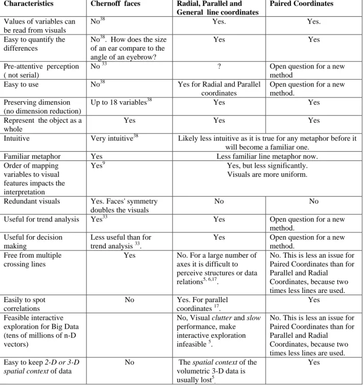
Below in Table 3 we compare characteristics of the Paired Coordinates with an icon-based technique of Chernoff faces and other line coordinates such as Parallel and Radial coordinates. Chernoff faces are multi-part glyphs in the shape of a human face and the individual parts, such as eyes, ears, mouth and nose represent the data variables by their shape, size and orientation8.
Table 3. Comparison of Paired and other line coordinates with Chernoff faces
Characteristics Chernoff faces Radial, Parallel and
General line coordinates
Paired Coordinates
Values of variables can be read from visuals
No38 Yes. Yes.
Easy to quantify the differences
No38. How does the size of an ear compare to the angle of an eyebrow?
Yes Yes
Pre-attentive perception ( not serial)
No 33 ? Open question for a new
method Easy to use No38 Yes for Radial and Parallel
coordinates
Open question for a new method.
Preserving dimension (no dimension reduction)
Up to 18 variables38 Yes Yes
Represent the object as a whole
Yes Yes Yes
Intuitive Very intuitive38 Likely less intuitive as it is true for any metaphor before it will become a familiar one.
Familiar metaphor Yes Less familiar line metaphor now. Order of mapping
variables to visual features impacts the interpretation
Yes9 Yes, but less significantly.
Visuals are more uniform.
Redundant visuals Yes. Faces' symmetry doubles the visuals
No No
Useful for trend analysis Yes33 Yes Open question for a new
method. Useful for decision
making
Less useful than for trend analysis 33.
Yes Open question for a new method.
Free from multiple crossing lines
Yes No. For a large number of axes it is difficult to perceive structures or data relations5, 6,17.
No. This is less an issue for Paired Coordinates than for Parallel and Radial
Coordinates, because two times less lines are used. Easily to spot
correlations
No Yes. For parallel coordinates 17.
Yes
Feasible interactive exploration for Big Data (tens of millions of n-D vectors)
No, Visual clutter and slow
performance, make interactive exploration infeasible 5.
No. This is less an issue for Paired Coordinates than for Parallel and Radial
Coordinates, because two times less lines are used. Easy to keep 2-D or 3-D
spatial context of data
No The spatial context of the volumetric 3-D data is usually lost5.
The use of the faces is based on the human ability to easily recognize faces and small changes in them. However faces are not necessarily superior to other multivariate techniques33. In general, icons have advantages over other representations when there is a semantic relation between the icons and the task39. The arbitrary match of face features with attributes of the n-D vector has no such semantic match. The features of the faces such as the curvature of the mouth, the eye size and the density of the eyebrow are of different importance for our interpretations of the whole face13 and arbitrary match will lead to very different conclusion about of n-D vectors based on the facial metaphor.
Table 3 presents a comparison of Paired and other line coordinates with Chernoff faces that shows the advantages of line coordinates relative to Chernoff faces. There are multiple modifications of Radial and Parallel coordinates methods that intend to improve them. Most of these improvements are also applicable to the paired coordinates. Therefore we compare “apples to apples”, which is the basic Radial and Parallel coordinates with the basic Paired Coordinates.
5. CONCLUSION
Further development and application of parallel coordinates took multiple directions18 that include supporting unstructured datasets with millions of points, multi-timepoint volumetric datasets with tens of millions of points per timestep5 and exploration of large document corpora6. Parallel hierarchical coordinates6,17, Smooth parallel coordinate34,
Higher order parallel coordinates41, Continuous parallel coordinates18 have been developed as a way to deal with large
datasets and to decrease clutter from crossing lines. These methods include hierarchical data clustering, proximity-based coloring, and navigation tools to support data localization, smooth curves and others. Parametric parallel coordinates with axis of different length are proposed21. This work uses a color mapping function that through interactive adjustment reduces the influence of individual data on the overall data to achieve a better visualization. 3-D parallel coordinates have been developed in45. The X,Y plane represents a traditional parallel coordinates and Z coordinate is used to represent the density of the lines in 2-D. In7,43,44 parallel coordinates are combined with scatter-plot matrixes and histograms to produce multiple coordinated views. Parallel coordinates are combined with the statistical analysis visualizations40 to form Enhanced parallel coordinates. In all line and paired coordinates the ordering of the axes influences the shape of lines and their interpretation. A significant effort has been devoted to controlling the ordering and scaling parallel coordinates during the exploration so that the variables of interest can be studied in adjacent axes3.
Most of these approaches are applicable to the General Line Coordinates and to the Paired Coordinates and can be applied to develop their more advanced versions. The future work is exploring mathematical properties of the proposed visualization methods, developing their advanced versions and applying them to challenging datasets.
The fundamental novelty of the concept of the Paired Coordinates is that uses a single 2-D plot to represent n-D data as an oriented graph based on the idea of collocation of pairs of attributes with much less clutter than other methods produce. The main advantage of the General Line Coordinates and the Paired Coordinates is that they provide a common
framework that includes popular Parallel and Radial coordinates and generate a large number of new visual
representations of multidimensional data without dimension reduction.
6. REFERENCES
[1] Ahonen-Rainio, P., Kraak, M., “Towards Multivariate Visualization of Metadata Describing Geographic Information,” Exploring Geovisualization, Elsevier, Eds. J. Dykes, A. MacEachren, Menno-Jan Kraak, 611-626, (2005)
[2] Andrews, D., “Plots of high dimensional data,” Biometrics 28, 125-36, (1972)
[3] Andrienko, G., Andrienko, N., “GIS visualization support to the C4.5 classification algorithm of KDD,” Proceedings of the 19th International Cartographic Conference, 747-755, (1999)
[4] Bache, K., Lichman, M. “UCI Machine Learning Repository,” http://archive.ics.uci.edu/ml]. Irvine, CA, University of California, School of Information and Computer Science, (2013)
[5] Blaas, J., Botha, C., Post F., “Extensions of Parallel Coordinates for Interactive Exploration of Large Multi- Timepoint Data Sets,” IEEE Transactions on Visualization and Computer Graphics 14(6), 1436-1443, (2008)
[6] Candan, K.S., Di Caro, L., Sapino, M.L., “PhC: Multiresolution visualization and exploration of text corpora with parallel hierarchical coordinates,” ACM Trans. on Intelligent Systems and Technology 3 (2), article 22, (2012)
[7] Chen, Y., Cai, J.-F., Shi, Y.-B., Chen, H.-Q., “Coordinated visual analytics method based on multiple views with parallel coordinates,” Xitong Fangzhen Xuebao / Journal of System Simulation 25 (1), 81-86, (2013)
[8] Chernoff, H., “The use of faces to represent points in k-dimensional space graphically,” Journal of the American Statistical Association, Vol. 68, 361-68 (1973)
[9] Chuah, M., Eick, S., “Information rich glyphs for software management data,” IEEE Computer Graphics and Applications (1998)
[10] Cleveland, W., McGill, M., [Dynamic Graphics for Statistics], Wadsworth, Inc., (1988)
[11] Draper, D., “Challenger USA Space Shuttle O-Ring Data Set,” UC Irvine Machine Learning Repository, (1993) http://archive.ics.uci.edu/ml/machine-learning-databases/space-shuttle/]
[12] Draper, D., “Assessment and propagation of model uncertainty (with Discussion),” Journal of the Royal Statistical Society Series B, 57, 45-97, (1995)
[13] De Soete, G., “A perceptual study of the Flury-Riedwyl faces for graphically displaying multivariate data,” International Journal of Man-Machine Studies, 25(5), 549-555, ACM Press, (1986)
[14] Fienberg, S. E., “Graphical methods in statistics,” American Statisticians, 33, 165-178, (1979)
[15] Feiner, S., Beshers C., “Worlds within worlds: Metaphors for exploring n-dimensional virtual worlds,” In Proc. of the 3rd annual ACM SIGGRAPH symposium on User interface software and technology, 76-83, (1990)
[16] Fekete, J., Plaisant, C., “Interactive information visualization of a million items,” In: Proceedings of IEEE
Symposium on Information Visualization, (2002)
[17] Fua, Y., Ward, M.O., Rundensteiner, A., “Hierarchical parallel coordinates for exploration of large datasets,” Proc. of IEEE Visualization, 43-50 (1999)
[18] Heinrich, J., Weiskopf, D., “State of the Art of Parallel Coordinates,” EUROGRAPHICS 2013/ M. Sbert, L. Szirmay-Kalos, 95-116, (2013)
[19] Heinrich, J., Weiskopf, D., “Continuous Parallel Coordinates,” IEEE Transactions on Visualization and Computer Graphics, 15(6), 1531-1538, (2009)
[20] Hoffman, P., Grinstein, “A Survey of Visualizations for High-Dimensional Data Mining,” In: Information Visualization in Data Mining and Knowledge Discovery, Eds. U. Fayyad, A. Wierse, G. Grinstein, 44-82, Academic Press, (2002)
[21] Jiang, Z., Cheng, S., Meng, X., Zhang, Z., “Research on time-series data visualization method based on
parameterized parallel coordinates and color mapping function,” 2012 International Conference on Systems and Informatics, ICSAI 2012, article 6223048 , 510-514 , (2012)
[22] Inselberg, A., Dimsdale, B., “Parallel coordinates: A tool for visualizing multidimensional geometry,” Proc. of Visualization ’90, 361-78, (1990)
[23] Inselberg, A., [Parallel Coordinates: Visual Multidimensional Geometry and its Applications], Springer, 2009. [24] Jolliffe, J., [Principal of Component Analysis], Springer Verlag, (1986)
[25] Keim, D., Hao, M., Dayal, U., and Hsu M., “Pixel bar charts: a visualization technique for very large multi-attribute data sets,” Information Visualization, 1(1): 20–34, (2002)
[26] Kohonen, T., “The self-organizing map,” Proc. of IEEE, 1464-80, (1978)
[27] Kovalerchuk, B., Schwing, J. (Eds), [Visual and Spatial Analysis: Advances in Data Mining], Reasoning, and Problem Solving, Springer, (2005)
[28] Kovalerchuk, B., Delizy, F., Riggs, L., Vityaev, E., “Visual Discovery in Multivariate Binary Data,” SPIE Visualization Conference, Vol. 7530: J.Park; M, C. Hao; P.C. Wong; C. Chen, Eds, 75300B, (2010)
[29] Kovalerchuk, B., Delizy, F., Riggs, L., “Visual Data Mining and Discovery with Binarized Vectors,” In: Data Mining: Foundations and Intelligent Paradigms, 24: 135-156, Springer, (2012)
[30] Kruskal, J., Wish M., [Multidimensional Scaling], Sage Publications, (1978)
[31] LeBlanc, J., Ward M., and Wittels, N., “Exploring n-dimensional databases,” Proc. of Visualization ’90, 230-237, (1990)
[32] Mead, A., “Review of the development of multidimensional scaling methods,” The Statistician, 33, 27-35, (1992)
[33] Morris, C., Ebert, D., and Rhengans, P., “An experimental analysis of the pre-attentiveness of features in Chernoff Faces,” In: Proceedings of Applied Imagery Pattern Recognition: 3D Visualization for Data Exploration and Decision Making, (1999)
[34] Moustafa, R., Wegman, E., “On some generalization to parallel coordinate plots,” In: Seeing a Million – A Data Visualization Workshop, 41–48, (2002)
[36] Novotny, M., “Visually Effective Information Visualization of Large Data,” In: 8th Central European Seminar on
Computer Graphics, 41-48, CRC Press. http://www.vrvis.at/TR/2004/TR_VRVis_2004_006_Full.pdf, (2004)
[37] Ribarsky, W., Ayers E., Eble J., Mukherjea S., “Glyphmaker: Creating customized visualization of complex Data,” IEEE Computer, 27(7), 57-64, (1994)
[38] Schroeder, M., “Intelligent Information Integration: From Infrastructure through Consistency Management to Information Visualization,” In: Exploring Geovisualization, Elsevier, Eds. Jason Dykes, Alan M. MacEachren, Menno-Jan Kraak , 477-494, (2005)
[39] Spence, R., [Information Visualization], Harlow, London: Addison Wesley/ACM Press Books, 206 pp., (2001) [40] Steed, C., Fitzpatrick P., Swan J. E. II, and Jankun-Kelly T.J., “Tropical Cyclone Trend Analysis using Enhanced Parallel Coordinates and Statistical Analytics,” Cartography and Geographic Information Science, 36(3), 251- 265, (2009)
[41] Theisel, H., “Higher order parallel coordinates,” In: Proc. of the 5th Fall Workshop on Vision, Modeling, and Visualization, 415–420, Saarbrucken, Germany (2000)
[42] Tufte, E., [Visual Expiation], Graphics Press, (1997).
[43] Viau, C., McGuffin, M.J., Chiricota, Y., Jurisica, I. “The FlowVizMenu and parallel scatterplot matrix: Hybrid multidimensional visualizations for network exploration,” IEEE Transactions on Visualization and Computer Graphics, 16 (6), 1100-1108, (2010)
[44] Yuan, X., Guo, P., Xiao, H., Zhou, H., Qu, H., “Scattering points in parallel coordinates,” IEEE Transactions on
Visualization and Computer Graphics, 15 (6), 1001-1008, (2009)
[45] Wang, H., Song, Z., Jing, K., Zhang, L., “Research on methods to improve parallel coordinates visualization,” Applied Mechanics and Materials 303-306 , 1618-1625, (2013)
[46] Wegman, E., “Hyperdimensional data analysis using parallel coordinates,” Journal of the American Statistical Association, 411(85), 664, (1990)
[47] Weinberg, S., “An introduction to multidimensional scaling,” Measurement and evaluation in counseling and \
development, 24, 12-36, (1991)
[48] Wong, P., Bergeron R.D., “30 Years of Multidimensional Multivariate Visualization,” In: G. M. Nielson, H. Hagan, and H. Muller (Eds), Scientific Visualization - Overviews, Methodologies and Techniques, 3-33, IEEE