Automatic Video Captioning using Deep Neural Network

Rochester Institute of Technology Rochester Institute of Technology

RIT Scholar Works

RIT Scholar Works

4-2017

Automatic Video Captioning using Deep Neural Network

Automatic Video Captioning using Deep Neural Network

Thang Huy Nguyen [email protected]

Follow this and additional works at: https://scholarworks.rit.edu/theses

Recommended Citation Recommended Citation

Nguyen, Thang Huy, "Automatic Video Captioning using Deep Neural Network" (2017). Thesis. Rochester Institute of Technology. Accessed from

This Thesis is brought to you for free and open access by RIT Scholar Works. It has been accepted for inclusion in Theses by an authorized administrator of RIT Scholar Works. For more information, please contact

Automatic Video Captioning using Deep Neural Network

Master’s Thesis

Thang Huy Nguyen

A Thesis Submitted in Partial Fulfillment of the Requirements for the Degree of Master of Science in Computer Engineering

Supervised by Dr. Raymond Ptucha

Department of Computer Engineering Kate Gleason College of Engineering

Rochester Institute of Technology Rochester, NY

04/2017

Approved By:

_____________________________________________Date:______________ Dr. Raymond Ptucha

Primary Advisor – R.I.T. Dept. of Computer Engineering

_____________________________________________Date:______________ Dr. Nathan Cahill

Secondary Advisor – R.I.T. School of Mathematical Sciences

_____________________________________________Date:______________ Dr. Dhireesha Kudithipudi

Acknowledgements

I would like to thank professor Ptucha, my amazing mentor, who has always motivated, encouraged and given me valuable advice throughout the research. I would like to thank my colleague Shagan Sah for his feedback and his help to this work. Finally, I would like to thank Machine Intelligence Lab of Rochester Institute of Technology for providing me necessary resources to complete this project.

Abstract

Video understanding has become increasingly important as surveillance, social, and informational videos weave themselves into our everyday lives. Video captioning offers a simple way to summarize, index, and search the data. Most video captioning models utilize a video encoder and captioning decoder framework. Hierarchical encoders can abstractly capture clip level temporal features to represent a video, but the clips are at fixed time steps. This thesis research introduces two models: a hierarchical model with steered captioning, and a Multi-stream Hierarchical Boundary model. The steered captioning model is the first attention model to smartly guide an attention model to appropriate locations in a video by using visual attributes. The Multi-stream Hierarchical Boundary model combines a fixed hierarchy recurrent architecture with a soft hierarchy layer by using intrinsic feature boundary cuts within a video to define clips. This thesis also introduces a novel parametric Gaussian attention which removes the restriction of soft attention techniques which require fixed length video streams. By carefully incorporating Gaussian attention in designated layers, the proposed models demonstrate state-of-the-art video captioning results on recent datasets.

Table of

Contents

1.2 MOTIVATION FROM PREVIOUS WORK ... 12

CHAPTER 2 CONVOLUTIONAL NEURAL NETWORK ... 14

2.1 CONVOLUTIONAL LAYER ... 15

2.2 POOLING LAYER ... 17

2.3 ACTIVATION FUNCTIONS ... 18

2.4 COMMON CNNARCHITECTURES ... 19

CHAPTER 3 RECURRENT NEURAL NETWORKS ... 20

3.1 VANILLA RECURRENT NEURAL NETWORK ... 21

3.1.1 BACK PROPAGATION THROUGH TIME ... 23

3.1.2 VANISHING AND EXPLODING GRADIENTS PROBLEM ... 25

3.2 LONG-SHORT TEM MEMORY NETWORK ... 27

3.3 RECURRENT HIGHWAY NETWORK ... 29

CHAPTER 4 VIDEO CAPTIONING ... 31

4.1 ENCODER-DECODER MODELS ... 34

4.2 SOFT ATTENTION ... 37

CHAPTER 5 METHODOLOGY ... 39

5.1 GAUSSIAN ATTENTION ... 40

5.2 ATTENTION STEERING ... 43

5.3 VIDEO2VEC REPRESENTATION ... 45

5.4 SHOT BOUNDARY DETECTION ... 47

5.5 MULTI-STREAM HIERARCHICAL BOUNDARY MODEL ... 48

5.6 GAUSSIAN STEERING MODEL ... 50

5.7 LOSS FUNCTION ... 51

CHAPTER 6 DATASET AND TRAINING DETAILS ... 53

6.2 TRAINING DETAILS ... 54

6.3 BEAM SEARCH ... 55

CHAPTER 7 EVALUATION METRICS ... 57

7.1 BLEU ... 58

7.2 METEOR ... 60

7.3 CIDER ... 62

7.4 ROUGE-L ... 64

CHAPTER 8 RESULTS AND DISCUSSION ... 65

8.1 MHB RESULTS ... 65

8.2 HGA RESULTS ... 68

8.2.1 PERFORMANCE ON MSVD ... 68

8.2.2 PERFORMANCE ON MSRVTT ... 70

8.3 LOSS CURVES ... 74

8.4 ANALYSIS OF GAUSSIAN ATTENTION ... 76

8.5 SAMPLE CAPTION ... 83

8.5.1 MHB MODEL ... 83

8.5.2 BASELINE(GA-5)+HGA MODEL ... 84

CHAPTER 9 CONCLUSION AND FUTURE WORK ... 86

List of

Figures

FIGURE 1 HIGH-LEVEL VISUALIZATION OF A CONVOLUTIONAL NEURAL NETWORK ... 14

FIGURE 2 AN EXAMPLE OF INPUT VOLUME IS COMPUTED IN THE FIRST CONVOLUTIONAL LAYER 16 FIGURE 3 EXAMPLE FILTERS LEARNED BY ALEXNET ... 16

FIGURE 4 EXAMPLE OF A POOLING LAYER ... 17

FIGURE 5 ILLUSTRATION OF RELU FUNCTION ... 18

FIGURE 6 VANILLA RNN ... 21

FIGURE 7 AN UNFOLDING IN TIME RECURRENT NEURAL NETWORK ... 22

FIGURE 8 A SIMPLE RNN ... 23

FIGURE 9 INSIDE LSTM MODULE ... 27

FIGURE 10 SCHEMATIC OF AN RHN LAYER INSIDE THE RECURRENT LOOP. ... 29

FIGURE 11 MEAN-POOL ARCHITECTURE ... 34

FIGURE 12 S2VT ARCHITECTURE ... 35

FIGURE 13 STACKED LSTM VIDEO ENCODER ... 35

FIGURE 14 HRNE MODEL ... 36

FIGURE 15 HIGH-LEVEL VISUALIZATION OF SOFT ATTENTION TO VIDEO DESCRIPTION GENERATION ... 37

FIGURE 16 ILLUSTRATION OF THE PARAMETERIZED GAUSSIAN ATTENTION MODEL FOR STEERING THE TEMPORAL ALIGNMENT BETWEEN THE VIDEO AND WORD SEQUENCE ... 42

FIGURE 17 ATTENTION STEERING USING NORMALIZED TEMPORAL FEATURE RELEVANCE ... 44

FIGURE 18 OVERVIEW OF THE MULTI-STREAM HIERARCHICAL BOUNDARY MODEL FOR VIDEO CAPTIONING ... 49

FIGURE 19 OVERVIEW OF GAUSSIAN STEERING MODEL FOR VIDEO CAPTIONING ... 50

FIGURE 20 EXAMPLE OF SELECTING WORDS AT EACH TIME STEP ... 56

FIGURE 21 FINAL CANDIDATE SENTENCES ... 56

FIGURE 22 EXAMPLE BOUNDARY ATTENTION VECTOR WHERE THE DIPS INDICATE VIDEO BOUNDARIES IN [0 − 1] NORMALIZED VIDEO ... 67

FIGURE 26 LOSS VALUE OF GA-5 MODEL OVER ITERATIONS. ... 74

FIGURE 26 LOSS VALUE OF HGA MODEL OVER ITERATIONS. ... 74

FIGURE 26 LOSS VALUE OF MHB MODEL OVER ITERATIONS. ... 75

FIGURE 26 GAUSSIAN ATTENTION VISUALIZATION FOR SAMPLE VIDEOS FROM MSVD ... 77

FIGURE 27 COMPLEX CLIP COMBINED FROM 3 TOTALLY DIFFERENT CLIPS ... 78

FIGURE 28 COMPLEX CLIP COMBINED FROM 3 TOTALLY DIFFERENT CLIPS ... 80

FIGURE 29 SAMPLE CAPTIONS FOR MHB MODELS ... 83

FIGURE 30 SAMPLE CAPTIONS FOR BASELINE MODEL(GA-5) ... 84

List of Tables

Table 1. Video-sentence pair dataset statistics. ... 53

Table 2. A summary of the evaluation metrics. ... 57

Table 3. BLEU score computation example ... 59

Table 4. MSVD caption evaluation results with MHB model. ... 65

Table 5. MSR-VTT results on held-out test set. ... 66

Table 6 Comparison of captioning results on MVAD dataset. ... 67

Table 7 MSVD caption evaluation results on the held-out test set. ... 69

Table 8 HGA results on the held out MSR-VTT test set. ... 70

Table 9 MSR-VTT results on the held-out test set. We compare with recent entries in the MSR Video to Language Challenge. ... 72

Table 10 Comparing Gaussian attention at different layers for MSR-VTT test set. Adding GA show clear improvement over SA and attention is most important at the word generation layer. ... 73

Table 11 Performance evaluation with number of Gaussian filters 532 for attention on the MSVD test set. ... 76

Table 12 Illustration of Gaussian shape correspond with word in the caption sentence. . 79

Chapter 1

Introduction

Deep learning has recently revolutionized computer vision in many applications. By learning deep features and representations, a machine can match or even beat human performance in various tasks such as image classification, object recognition, and video segmentation. However, tasks like image and video captioning still remain a challenge and have captured an immense attention from literature in the past two years. The nature of a video stream with high temporal dependencies, multiple scenes in a complex video and diverse kinds of objects and actions make captioning very difficult. Yet, despite this, many architectures and methods have been proposed which substantially push forward research in video description. Building upon those successes, this thesis work develops robust captioning frameworks which can automatically generate captions for both simple and complex videos.

1.1 Novel Contributions

• Gaussian parametric attention: Soft attention models have an intrinsic limitation that all input buffers need to be of the same duration. This is because the attention vector is associated with a learnable, but fixed dimension weight matrix. For videos, this requires cropping longer videos or padding shorter videos. The proposed parametric Gaussian attention model removes this limitation by applying a continuous, rather than discrete weight distribution.

• Temporal steering. Existing attention models are guided by temporal features of the training data. For example, when the phrase winning goal occurs, the attention might jump towards the end of video. The introduced temporal attention steering mechanism uses frame level visual concepts to guide attention based on current video properties (detection of objects, activities, etc.) and not on training data trends.

• Introduction of an intelligent hierarchy for encoding a video. This hierarchy is based on intrinsic video boundaries. We refer to this as a Multi-stream Hierarchical Boundary (MHB) model, and further adapt Recurrent Highway Networks for the captioning task.

• We train fully end-to-end models that learns from video features to determine the temporal bounds of video clips to generate text descriptions of an entire video and demonstrate state-of-the-art captioning results on recent video datasets.

1.2 Motivation from previous work

Image and video understanding has gained a lot of attention in deep learning research recently. Image classification [1-4], object detection [5, 6], semantic segmentation [7-9], image captioning [10-12], and localized image description tasks [13] have witnessed tremendous progress in the last few years.

Automatically describing videos with natural language text enables more efficient search and retrieval, can aid visual understanding in the medical, security, and military applications, and can even be used to describe pictorial content to the visually impaired. Attention models learn to select the most relevant segments that associate with the text.

Spatial [14], temporal [15] [16, 17] and attribute [18] based attention models strive to localize objects in image frames, actions in videos or attend to specific word attributes. The ability to understand how well temporal attention works on video is limited given that most of the popular datasets are comprised of short videos. For example, the average video duration of the MSVD [19] YouTube clips is 10.2 seconds and the average duration of M-VAD [20] movie descriptions clips is 5.8 seconds.

`

Current methods for generating attention weights are determined by hard training statistics, not by visual concepts. For example, if training videos often end with humans fails, the model may learn to associate end of video as it predicts the words “falls down”.

If a video and corresponding caption are “woman scares man skateboarding and he falls down”, the attention model would perform as expected. But if the caption is “man falls down and then does great skateboard trick”, the trained attention parameters would perform poorly as the model would seek attention over the wrong temporal location in the video. To steer the attention mechanism to the proper region in the video, our model extracts frame-wise temporal concepts across the length of the video. This enables the model to correlate specific words such as woman, man, and skateboarding, with region-specific locations across the video.

To steer attention towards appropriate spatio-temporal locations in a video, attention models weigh some regions high and others low. The model learns how to linearly combine multiple regions of a video by applying a convex combination of each. As weights are learned parameters, and parameters need to be fixed at train time, attention models are constrained such that all samples have equivalent number of regions. To enable the attention mechanism to be independent of video duration, we present parametric Gaussian attention models which learn a continuous function and samples this function at each discrete region.

Chapter 2

Convolutional Neural Network

Convolution neural networks (CNNs) are a special type of neural network which focus on data that has grid-like topology. CNNs have been extremely successful in practical applications and are adapted in many architectures such as: image recognition, object detection, object segmentation [1, 3, 4]. By combining multiple blocks and using small filter sizes, CNNs can learn an in-depth representation of input, thus make it surpass all other traditional methods in image-related tasks. To fully understand how CNNs work, we need to investigate certain operations that every Convolutional Neural Network has: convolution, pooling, and activation functions.

2.1 Convolutional layer

The convolutional layer is core building block of a Convolution Neural Network (CNN). In this layer, most of the computational operations are conducted. Each convolutional layer using a numerous number of small sized sliding windows (also called as kernels, filters or feature detector), multiply with the input element-wise to get the full convolution. For example, in Figure 2, the input is an RGB CIFAR-10 image with the size of 32´32´3. If this image were convolved with 16 filters with size of 5´5´3 and stride of 1 at the first layer, the output of 28´28´16. To make the output dimension the same as the input dimension, the images are often padded with zeroes. The depth, stride and number of zero padding are three hyperparameters in a convolutional layer that control the output volume. The depth is the number of filters we would like to choose, where each filter will learn some features from the input. The stride controls how the filter will slide through the input, the larger of the stride the smaller of the output spatially. Zero-padding is employed in some cases, mostly to preserve the size of input volume.

As [21] suggests, we can calculate the output of a convolutional layer as follow: • Assume we have input of 𝑊_"×𝐻_"×𝐷_"

• Hyperparameters:

o Number of filters K

o Each filter has spatial extent F o Stride is S,

o Number of padding P

o 𝑊_& = (𝑊_"− 𝐹 + 2𝑃)/𝑆 + 1 o 𝐻_& = (𝐻_"− 𝐹 + 2𝑃)/𝑆 + 1 o 𝐷_& = 𝐾

Figure 2 An example of input volume(32x32x3 CIFAR-10 image) is computed in the first convolutional layer[21]

Figure 3 shows the visualization of the first convolutional layer in the Alexnet[1] model. There are total 96 filters, each has size of 11´11´3, we can observe that in this layer the model is able to learn filters which have Gabor-like features.

Figure 3 Example filters learned by Alexnet. Each of the 96 filters shown here is of size [11x11x3], and each one is shared by the 55*55 neurons in one depth slice[21]

2.2 Pooling layer

Pooling layers are periodically inserted after each convolutional layer to reduce the dimensionality of the network.

Figure 4 Example of a pooling layer.[21]

Generally, the pooling layer take: • Input with size 𝑊"×𝐻"×𝐷" • With hyperparameters:

o Spatial extent F o Stride S

• Will produce output 𝑊_&×𝐻_&×𝐷_&, with:

o 𝑊_& = (𝑊_"− 𝐹)/𝑆 + 1 o 𝐻_& = (𝐻_"− 𝐹)/𝑆 + 1 o 𝐷_& = 𝐷_"

In the example in Figure 4 , the input has size of 224´224´64. After pooling with F=2,

S=2, the output has volume of size 112´112´64. The most common technique for pooling is max-pooling [1, 3, 4]. However, [22] suggests that in large scale networks, max-pooling can be substituted with convolutional layer with increased stride without loss in accuracy.

2.3 Activation Functions

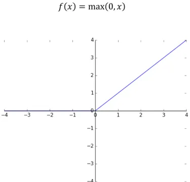
To model complex functions, neural networks insert non-linear activation functions between each layer. Many non-linearity activation functions have been proven effective since neural networks were introduced, such as: sigmoid function, tanh function, and Rectified Linear Unit (ReLU) function. The ReLU is the method of choice for most current architectures. The ReLU function computes the function:

𝑓 𝑥 = max 0, 𝑥 1

Figure 5 Illustration of ReLU function.

ReLU is very popular since [1] found out that it helped stochastic gradient descent converge much faster (a factor of six) than the tanh function. This can be attributed to its linear, non-saturated form. Moreover, ReLU has a simplistic implementation which does not involve expensive computations like sigmoid/tanh functions.

2.4 Common CNN Architectures

Several CNN architectures have been proposed and shown to be effective in real-world applications:

• LeNet [23]: The first successful convolution neural network by Yann Lecun.

• Alexnet [1] : This is the work popularized the convolutional networks, proposed by Alex Krizhevsky, Ilya Sutskever and Geoff Hinton.

• GoogLeNet [3] : ILSVRC 2014 winner, by introducing an Inception module, this architecture drastically reduces the number of learnable parameters. Interestingly, they replace the fully connecter layer with average pooling at the top of the network.

• VGGnet [2]: This model achieved second place in ILSVRC2014. This architecture has proved that the depth of the network is more important than breadth for a successful model.

• ResNet: Developed by Kaiming He et al.[4], winner of ILSVRC 2015. This is the model which obtains state of the art performance. It introduces skip connections with substantial use of batch normalization. In this thesis, most of our models use ResNet to facilitate our Recurrent Neural Networks layer to achieve the best results.

Chapter 3

Recurrent Neural Networks

Recurrent Neural Networks (RNNs) are types of neural networks that can process sequential data. While CNNs mostly focus on processing on fixed data at a time with a grid of values such as images, RNNs particularly handle data with temporal dependencies (data input changes over time). In theory, RNNs can handle arbitrary sizes of input and output, enabling the development of flexible neural network models.

Recently RNNs have been used in a wide variety of applications such as speech recognition, language modeling, image captioning, and video descriptions. In this research, we utilize two variants of RNNs, namely LSTM and RHN.

3.1 Vanilla recurrent neural network

To explain how RNNs work, first let’s examine a simple Recurrent Neural Network, here namely Vanilla Recurrent Neural Network. The idea of RNNs is to learn dependencies of input sequences. In RNNs, the input to the next step depends on previous computation (Figure 6).

Figure 6 Vanilla RNN. [24]

Assume we have input 𝑥_; at time t. The hidden state ℎ_; at t can be computed as:

ℎ_;= 𝑓 𝑈𝑥_;+ 𝑊ℎ_;>" 2

with f is non-linear function like tanh or ReLU.

Then we can calculate output at step t. Assume we need to predict the next word of a sentence. We have to calculate the probabilities for an entire dictionary of words:

By unfolding the network in Figure 6, we have the unrolled network as illustrated in Figure 7.

3.1.1 Back propagation through time

Figure 8 A simple RNN. [24]

Back propagation through time is the main technique used to train an RNN model. Assume we need to train a model for a machine translation application, our hidden state and output are defined as (4) and (5):

𝑠_;= tanh 𝑈𝑥_;+ 𝑊𝑠_;>" 4

𝑦_; = 𝑠𝑜𝑓𝑡𝑚𝑎𝑥 𝑉𝑠_; 5

Our loss function described by cross entropy loss:

𝐸_; 𝑦_;, 𝑦 = −𝑦_;𝑙𝑜𝑔𝑦_; 6

𝐸 𝑦, 𝑦 = 𝐸_; 𝑦_;, 𝑦_; = − 𝑦_;𝑙𝑜𝑔𝑦_;

; ;

where 𝑦_; is the correct word at time step t, 𝑦_; is our prediction. To calculate gradients, we use chain rule of differentiation. Assume we want to calculate gradients with respect to learning parameters U, V and W at loss 𝐸_Q:

𝛿𝐸Q 𝛿𝑉 = 𝛿𝐸Q 𝛿𝑦Q 𝛿𝑦Q 𝛿𝑉 8 =𝛿𝐸Q 𝛿𝑦Q 𝛿𝑦Q 𝛿𝑧Q 𝛿𝑧Q 𝛿𝑉 = (𝑦Q − 𝑦Q) ⊗ 𝑠Q 𝛿𝐸Q 𝛿𝑊 = 𝛿𝐸Q 𝛿𝑦Q 𝛿𝑦Q 𝛿𝑠Q 𝛿𝑠Q 𝛿𝑊 9 = 𝛿𝐸Q 𝛿𝑦Q 𝛿𝑦Q 𝛿𝑠Q 𝛿𝑠Q 𝛿𝑠W 𝛿𝑠W 𝛿𝑊 Q WXY

3.1.2 Vanishing and exploding gradients problem

The vanishing and exploding gradients are a common problem when training RNN models. Due to the propagation of derivatives across several time steps, repeated multiples of values less than one tend towards zero while repeated multiples of values above one explode. RNNs require derivatives to be repeatedly multiplied over times steps, thus being susceptible to vanishing and exploding gradients. As per (8), the notion Z[\

Z[] is a chain rule,

too. We can rewrite (8) as:

𝛿𝐸_Q 𝛿𝑊 = 𝛿𝐸_Q 𝛿𝑦_Q 𝛿𝑦_Q 𝛿𝑠_Q Q WXY 𝛿𝑠_^ 𝛿𝑠_^>" Q ^XW_" 𝛿𝑠_W 𝛿𝑊 10 Notice that _Z[Z[` `ab Q

^XW_"

is a product of Jacobian matrices with point-wise derivatives

since each element derivative is a vector function with respect to a vector. As proved by Pascanu et al. [25], on certain conditions each of these matrices can have an upper and lower bound of 1. If they have upper bound of 1, the product of those matrices go to 0 exponentially fast with the small values in the matrix and long-range dependencies (normal RNNs architectures have high number of time steps, such as in this research caption decoder has l=35). This leads to vanishing gradients and thus the model cannot learn the long-term dependencies. Vice versa, if those Jacobian matrices have a lower bound of 1, we have the exploding gradients problem. However, exploding gradients are easy to find

out: the loss becomes NaN (Not a Number) and we can efficiently avoid it by clipping gradients to a fixed constant, such as 5.0.

3.2 Long-Short Tem Memory Network

Figure 9 Inside LSTM module. [24]

To mitigate vanishing and exploding gradients problem as discussed in 3.1.2, Hochreiter et al. [26] proposed the Long Short-Term Memory (LSTM) architecture. The core idea behind LSTMs are cell states and gates. There are three gates in an LSTM which monitor the information flow through the cell: the forget gate, input gate and output gate.

The forget gate controls what information will be ignored from the cell state. The sigmoid activation (10) will output a value between 0 and 1, with 1 is “keep it” and 0 is “forget it”. We have 𝑓; computed by:

𝑓_;= 𝜎 𝑊_dℎ_;>"+ 𝑈_d𝑥_;+ 𝑏_d 11

with 𝜎 is sigmoid function, 𝑊d, 𝑈d, 𝑏d are learnable weight matrices and bias, ℎ;>" is the previous hidden state of LSTM cell, and 𝑥_; is the input vector.

The input gate 𝑖_; determines what information will be stored in the cell state. At first, a sigmoid function will decide the values will be updated:

𝑖;= 𝜎 𝑊gℎ;>"+ 𝑈g𝑥;+ 𝑏g 12

(𝑊_g, 𝑈_g, 𝑏_g are learnable weight matrices and bias) A memory cell state 𝐶; at time t is computed by:

𝐶_; = tanh 𝑊_i𝑥_;+ 𝑈_iℎ_;>"+ 𝑏_i 13

(𝑊_j, 𝑈_j, 𝑏_j are learnable weight matrices and bias)

The memory cell state 𝐶_; at time t is updated. The forget gate is multiplied by the forget gate with old state, resulting in the old state with information needed to be forget. Then we add the new candidate value which is scaled by input gate 𝑖_;∗ 𝐶_;:

𝐶_;= 𝑖_;∗ 𝐶_;+ 𝑓_;∗ 𝐶_;>" 14

Equation (14) is the key to alleviating the vanishing gradient problem in RNNs. The derivative from 𝐶; to 𝐶;>" is the value of the forget gate, and the error at 𝐶; can pass back to 𝐶_;>" without loss with no repeated weight matrix multiplication. This is referred to as Constant Error Carousel [26].

Finally, we decide what we will output to by output gate 𝑜; , then deliver the output hidden state ℎ_;:

𝑜;= 𝜎 𝑊l𝑥;+ 𝑈lℎ;>"+ 𝑏l 15

ℎ; = 𝑜;∗ tanh 𝐶; 16

3.3 Recurrent Highway Network

Figure 10 Schematic of an RHN layer inside the recurrent loop. [27]

Vanishing and exploding gradients are not the only problem with the traditional RNN architectures. Training recurrent networks by stacking many layers to create depth is difficult. Intuitively, training a deep recurrent neural network can gain better accuracy but requires huge space and time trade-off. Recently, Zilly et al. [27] introduced Recurrent Highway Networks (RHNs) with the ability to train deeper models with less parameters. A RHN cell is comprised of multiple highway layers, each with two gates- the transform and carry gates. Given an input 𝑥[;]_{, 𝑡 is the current time step, the output of a RHN is described} as:

ℎ_u; = tanh 𝑊_v𝑥; _𝛪 uX" + 𝑅vy𝑠u>" ; _{+ 𝑏} vy 18 𝑡_u; = tanh 𝑊_z𝑥;_Ι uX" + 𝑅zy𝑠u>" ; _{+ 𝑏} zy 19 𝑐_u; = tanh 𝑊_j𝑥;_𝛪 uX" + 𝑅jy𝑠u>" ; _{+ 𝑏} jy 20

where, 𝑙 denotes recurrent depth of RHN; ⊙ is element-wise function; Ι_{} is indicator function; 𝑊_v,z,j ∈ 𝑅€•‚ _{and 𝑅}

vy,zy,jy ∈ 𝑅€•€ are transform weight matrices and 𝑏_vy,zy,jy ∈ 𝑅€ _{is the bias. It can be observed that RHN conceptually is a variant of LSTM} if 𝑙 = 1, but RHN layers are designed to expand with 𝑙 > 1, thus enabling complex state transitions which lead to better remembering, forgetting or carrying information. Proved by [27], this design promises to be a better method to train deep recurrent networks while still alleviating the vanishing/exploding gradients problem.

In this research, we incorporate a variant of Recurrent Highway Networks to evaluate its performance against LSTM.

Chapter 4

Video captioning

The success of deep learning in the still image domain has influenced research in the video understanding domain, including video captioning. Early work on video captioning relied on extracting semantic content such as subject, verb, object, and associating it with the visual elements [28-30]. For instance, [29] form a Factor Graph Model to obtain the probability for the semantic content and then use a search based optimization to get the best combination of subject, verb and object to fit in a sentence template. Earlier works were also limited to activity or context specific videos with a small vocabulary of objects and activities. With the availability of large video-sentence pair datasets with rich language information, recent studies [10, 31] have demonstrated use of neural networks to directly model language conditioned on video. Deep neural network architectures for video classification are now prevalent [32, 33].

Initial works that introduced recurrent neural networks for video captioning used a mean pooled feature as the video representation [31]. An alternate approach uses an encoder-decoder [34] framework that first encodes f frames, one at a time to the first layer of a two layer Long-Short-Term Memory (LSTM), where f can be of variable length. This latent representation is decoded into a natural language sentence one word at a time, feeding the output of one time step into the second layer of the LSTM in the subsequent time step. This has been shown in S2VT [35] .

Attention mechanisms were initially proposed in [36] and used in the video captioning context by [16]. This allows the selection of relevant temporal segments of a video conditioned on the text-generating recurrent network. Spatial attention over parts of an image is shown by [14]. They use the outputs of the last convolution layer to guide the word generation to look into specific parts of image. They also present a hard-attention mechanism equivalent to reinforcement learning with the reward for selecting the image region proportional to the target sentence. Semantic attention was used to enhance image captioning by independently selecting a list of word attributes [18]. Similarly, [37] and [38] have included video attributes or tags to help generate improved captions. The attribute or tag selection is not trained along with the language model and it becomes challenging to obtain rich attributes or “concepts” for videos that can also categorize actions along with objects.

More recently, video captioning was extended to paragraph generation using independent recurrent networks at the word and sentence level [17]. Hierarchical recurrent networks have also been used to encode the video in an embedding before generating words [15]. They also apply the attention over multiple stages (local, regional and global) which increases the number of learnable parameters.

All described methods are dependent on availability of large scale datasets with video-sentence paired data. [39] demonstrated the use of knowledge transfer from independent language and image data for image captioning. This thesis is loosely inspired by this study in terms of using sentence independent visual concepts to improve the quality of generated

captions. In contrast to traditional soft attention, our model guides the attention using independent temporal “concepts” of the video.

Our work is additionally inspired by the soft attention model for video captioning presented in [16]. We augment it by parameterizing the attention mechanism with a Gaussian distribution over the video length. By learning the normalized mean and sigma values of the distribution, the model removes any dependency on the video duration. This also allows for temporal data augmentation to generate multiple sentences per video. Gaussian attention filters are discussed in [40] but the application is limited to activity classification and their equally spaced attention filters limit the use of attention for word generation.

4.1 Encoder-Decoder models

Initial works that introduced Recurrent Neural Networks (RNNs) for video captioning used a mean pooled [31] feature as the video representation as shown in Figure 11. In this work, the input to the LSTM layer is simply the average of all feature vectors:

𝜑 𝑉 =1 𝑛 𝑣g

€

gX"

21

Where 𝑣g is the output of the CNN encoder. By treating all feature vectors with the same importance and averaging them up like this, the mean pool approach limits the model’s capability in recognizing and exploiting the temporal dependencies between frames.

Figure 11 Mean-pool architecture. [31]

In the following work, Venugopalan et al. [35] introduce an encoder-decoder framework which encodes features from f frames of a video to the first layer of a two-layer LSTM to

form a latent embedding that is decoded into a natural language sentence by a second LSTM layer (Figure 12). The decoding is done by using the output word from the previous time step along with hidden vectors. One of the main advantages of the encoder-decoder model is the ability to handle variable length sequences.

Figure 12 S2VT architecture. [35]

Figure 13 Stacked LSTM video encoder. [15]

Pan et al. [15] discovered that by utilizing hierarchy in different stages as shown in Figure 14, their model can effectively learn complex temporal structure of video. This resulted in

higher captioning scores (METEOR, BLEU) in video captioning tasks. Instead of stacking several layers of LSTM (Figure 13), the input sequences (𝑥_", 𝑥_&, … , 𝑥_z) are divided into several chunks (𝑥_", 𝑥_&, … , 𝑥_€), (𝑥_{"_[}, 𝑥_{&_[}, … , 𝑥_{€_[}), … , (𝑥_{z>€_"}, 𝑥_{z>€_&}, … , 𝑥_z), where s

is stride which depicts the distance between two adjacent chunks. After feeding into the first LSTM filter, the output will be a sequence of feature vectors ℎ_", ℎ_&, . . . , ℎ_z/€ and input into second LSTM layer. The first layer acts as local temporal structure learner of each subsequence, while the second layer exploits the global temporal structure among subsequences. This method has proved to be extremely successful, yielding robust scores (METEOR, BLEU) in video captioning tasks [15].

4.2 Soft Attention

Figure 15 High-level visualization of soft attention to video description generation. [16]

A simple way to encode a video is by averaging pixels or features across all frames in the video. Most commonly, features are the output of a frame passed into an ImageNet pre-trained CNN. However, this video representation would reduce the model’s ability to learn temporal structure. To avoid this problem, Yao et al. [16] introduced soft attention mechanisms, which can focus on a subset of the input sequence at each time step. Soft attention uses a weighted combination of these frame-level features, where the weights are influenced by the word decoder. Assume we have a sequence of feature vector

𝑉 = {𝑣_", 𝑣_&, . . , 𝑣_€}, unnormalized relevance score 𝑒_g; _{of i}th _{temporal feature at decoder} time step t is computed by:

𝑒_g; _{= 𝑤}z_{tanh 𝑊}

‹ℎ;>"+ 𝑈‹𝑣g + 𝑏‹ 22

Where, ℎ_;>"is the hidden state at the previous time step of the decoder, 𝑣_g is the frame feature vector representation of the 𝑖;Œ _{frame, and 𝑤, 𝑊}

‹, 𝑈‹, 𝑏‹ are learned parameters. This can be interpreted as an alignment between the encoder and decoder sequence. It

allows the video encoder to selectively weigh on parts of the video. As the frame relevance score is computed using fixed dimension weight matrices, it restricts the exact number of frames in the video. Moreover, given that the average length of videos is only a few seconds in most datasets, it seems counter intuitive to have strong localized attention in such a short duration.

After relevance scores are computed, dynamic weights 𝛼_g(;)are obtained by normalizing them: 𝛼_g; = exp 𝑒g ; exp 𝑒_^; € ^X" 23

Then, the weighted sum of the temporal feature vectors is calculated:

𝜑_; 𝑉 = 𝛼_g; 𝑣_g

€

gX"

Chapter 5

Methodology

This research introduces two video captioning architectures with several techniques: 1. Gaussian attention which aims to replace the popular Soft Attention (4.2), with

advantages over SA such as fewer parameters and better captioning performance. 2. Attention steering aids the attention mechanism to boost the model’s performance 3. Shot boundary detection which enables flexible hierarchy of layers instead of a

fixed stride as discussed in 4.1

4. Hierarchical architecture with fixed strides, along with soft hierarchy techniques using shot boundary detection.

5.1 Gaussian Attention

We define the Gaussian Attention (GA) to remove restrictions with the generic soft attention mechanism. The relevance score that weighs the input sequence is modeled with a Gaussian distribution. At each time step, the decoder observes a filtered/weighted encoder sequence. GA weighs the input sequence based on the temporal location and the shape of the distribution is modeled by the mean and standard deviation. We adapt the function to compute a continuous relevance score 𝑒; _{across the entire input sequence 𝑋 =}

(𝑥_", 𝑥_&, . . . , 𝑥_‘) at decoder time step 𝑡 as:

𝑒; _{= 𝜋}

W𝛮 𝑋 𝜇W;, 𝛴W; –

WX"

25

Where, each GA is a Gaussian distribution with its unique mean 𝜇_W; _{and covariance matrix}

𝛴_W; _{at time t, 𝛮 is the number of Gaussians and 𝜋}

W is a mixing coefficient. The mixing coefficients are normalized to sum to one. The input features 𝑋 ∈ 𝑅—בט_{, where D is} the number of input modalities, F is the length of each sequence, and M is the dimension of each feature. For example, if the two input modalities of spatial domain and temporal domain are used, we can learn a unique set of Gaussians for each modality by setting 𝐷 = 2. By varying mixing coefficients, mean and covariance of basic Gaussians, the superposition can approximate any continuous function by using sufficient number of Gaussians. Hence with correct parameters, a GA model can achieve the same function as

soft attention. We choose to model independent Gaussians, and replace 𝛴_W; _{with a scalar} standard deviation, 𝜎; _{at each time t.}

Computing the parameters allows the filter to temporally adapt to decoder decisions. With the loss back-propagated at each time step, the mean value of the Gaussian learns to focus on relevant locations of the sequence. Similarly, the standard deviation can learn to extract information from a longer or shorter segment. Thus, the GA formulation makes it adaptive both in terms of location and range. Resource utilization can be optimized as the decoder need not necessarily compute attention over the entire input sequence. The mean and standard deviation are computed as:

𝜇; _{= ℘ 𝑊}

šℎ;>"+ 𝑈š𝑋 + 𝑏š 26

𝜎; _{= 𝑊}

›ℎ;>"+ 𝑈›𝑋 + 𝑏› 27

Where 𝑊_š, 𝑊_›, 𝑈_š, 𝑈_›, 𝑏_š, 𝑏_›, are learned weights. We use the activation ℘ 𝑠 = 𝑠

𝑠 + 𝑐 for the mean values to scale to range [0, 1] as the input sequence is normalized

temporally. The normalization allows the model to compute attention over sequences of varying length. It also reduces the number of learnable weights from 𝑅Œ•Œ _{to 𝑅}Œ•–_{, where}

h is hidden dimension size of decoder and 𝑁 ≪ ℎ. Like soft attention, the attention weights

𝛼_g; _{at time t for input X are obtained by normalizing the relevance scores. The input to the} decoder is a weighted sum of the input X using the attention at time t.

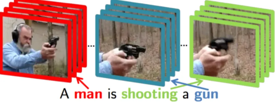
Figure 16 Illustration of the parameterized Gaussian attention model for steering the temporal alignment between the video and word sequence. The caption is generated using a recurrent neural network. For a video, the mean and standard deviation of the distribution is computed based on the outputs of the previous time steps (dotted lines). The curves depict change in the attention over the video based on the word generated in the caption generator.

Modeling the attention filter with a parametric distribution allows the decoder to view inputs with varying duration and hence it is better at exploiting the temporal structure of an input sequence. The parametric attention has the capability to sense the complete encoder sequence if required. This is important in a translation-like task where the generated word may hold relevance throughout the video. For example, after the word

“man” in Figure 16, the model learns to expand the attention to allow the caption generator to view the entire input as the associated visual feature of “man” appears in the entire video.

5.2 Attention steering

Traditional attention models are associated with a set of weight matrices that are learned during training. During test time, the weight matrices guide the attention and hence limit the attention mechanisms by prior training statistics. This is important as most video captioning datasets cannot possibly have a comprehensive representation of all activities and objects. If a certain semantic action/object like “cutting an apple” is more likely to appear in beginning of the video in the training set, the learned model may expect similar trends in test videos.

To obtain video specific attention, we both allow the network to “watch” the full video before attending to specific portions, and we introduce temporal concepts along the portions of the video. One way to encode a summary of an entire video can be done using an LSTM as shown in [35]. LSTMs have the capability to retain segments of the video but would have to remember both the context of the overall video and the relevant frames. With this restriction, it becomes difficult for the latent representation of the video (we use a dimension of 512) to have detailed attention, and surely would struggle for long videos. To overcome this restriction, we introduce temporal attention steering that guides the attention based on the feature statistics of the test video.

We further investigate the use of word label embeddings of objects present in video frames as temporal visual features. We use an ImageNet classifier trained on 4k classes [41] represented using a Glove [42] word embedding. Representing a large number of objects is important for “in-the-wild” videos. A bottom-up grouping strategy [41] is applied to the categories to deal with the problems of over-specific classes.

In reality, a sentence is described by both the objects and the whole scene as the context. Distinguishing individual objects from others in a scene, especially when there are multiple objects of different categories can be highly challenging. Hence, EdgeBox [43] is used to obtain proposal bounding box regions within each frame of a video. For the top 95% of all bounding boxes, we compute Glove word embedding of the ImageNet 4K CNN classes. These embedded word vectors are mean pooled to obtain a frame-level representation. We discover that the mean pooled class label embedding is rich in semantic information and is closer to the words in the ground truth sentence. Moreover, use of word embedding reduces the feature dimension from 4K to 300. This design choice reduces the number of learnable parameters substantially. As a complementary or alternative approach to temporal word concepts, one could use frame CNN features directly.

Figure 17 . Frame level features are weighted based on the relevance map and assists in guiding attention to video regions. 𝑊; and 𝑊;>" are words at times t and t-1, ℎ;>" is RNN hidden state.

5.3 Video2vec representation

In addition to the steering mechanism, an embedded vector representation of the entire video is input into the captioning model (right input in Figure 19). Just as word concepts capture the temporal object information, video level features (about the actions and activities in the video) are equally important. An embedding function 𝑓: 𝑉 → 𝑆 , that maps a video V with frames (𝑣_", 𝑣_&, . . . , 𝑣_€) into a representation 𝑆 is learned. We refer this transformation as Video2Vec.

Video2Vec-Activity: To learn powerful action and motion concepts, we use a recent activity classification dataset - ActivityNet [44], on human activity understanding that covers a wide range of complex daily activities. It is comprised of 849 video hours in over 200 activity classes. As these videos were collected from online video sharing sites they are excellent to transfer learned features for MSVD and MSR-VTT datasets which are also based on Youtube videos. The labeled videos are used to train a standard video-based activity classifier. We train two independent models using RGB (3- color channels) and optical flow inputs. Features before the loss layer are used as Video2Vec-Activity representation and we fine-tune the last fully-connected layer during caption generation.

Hierarchy over Gaussian Attention: As discussed in 4.1, the recently proposed hierarchical neural encoder [15] technique efficiently captures temporal dependencies in videos. Hence, we integrate it with our GA model and term it as Hierarchy over Gaussian Attention (HGA). The hierarchy of recurrent layers adds more non-linearity to the GA model. The hidden state of LSTM in layer l-1 at the last time step is the input to layer l.

This ensures easy back-propagation of loss compared with a simple layer stacking by reducing the number of steps the loss back-propagates. The first layer learns local temporal dynamics within short clips and the second layer learns the difference between these short clip sequences. The output at the last time step of the second layer is a vector representation for the entire video. We further adapt [15] by replacing soft attention with Gaussian attention between all recurrent layers.

5.4 Shot boundary detection

Features extracted from CNN models have proven to be useful in cut-transition boundary detection between two shots in a video stream [45]. Given 𝛼_g and 𝛼_^ are two CNN feature vectors of two consecutive frames, the cosine distance 𝛥 (𝑖, 𝑗) between them can be calculated as follows:

𝛥 𝑖, 𝑗 = cos 𝑎_g, 𝑎_^ = 𝑎g. 𝑎^

𝛼_g 𝛼_^ 28

𝛥 𝑖, 𝑗 ∈ [0,1], with higher values having higher probability of a boundary cut. For example, one could experimentally determine a threshold 𝜁 where a boundary exists when

𝛥 (𝑖, 𝑗) > 𝜁. Unlike Euclidean distance, the cosine distance needs no additional normalization steps. Xu et al. [45] determined this distance is effective in the cut-transition detection task. Our results concur and we employ it to detect the boundary to facilitate the soft hierarchy layer.

5.5 Multi-stream Hierarchical Boundary Model

Referring to Figure 18, the encoding stage takes in a given video stream, whereby the first layer takes in local features (𝑥_", 𝑥_&, . . . , 𝑥_€), and outputs two sequence vectors: 1) equal spaced (𝑤_", 𝑤_&, . . . , 𝑤_¥); and 2) clip level (𝑧_", 𝑧_&, . . . , 𝑧_¦). The equal spaced output layer gets 𝑝 outputs from first layer with 𝑝 = 𝑛/𝑘 (𝑛 is number of input features and 𝑘 is designed stride value). The clip level output layer utilizes information on shot boundaries guided by a learned vector based on the cosine distance:

𝑧_g = 𝑦_g . Δ 𝑖, 𝑗 . 𝑊_ª« + 𝑏_ª« 29

where 𝑊_ª« and 𝑏_ª« are learned weights and bias, 𝑦_g is output at each time step of first layer. As illustrated in Figure 18 the video is encoded through a combination of equally spaced and clip level feature representations. The fusion of local (frame) level, hierarchy (equally spaced) and clip (detected boundaries) level is input to the caption decoder. At each time step, the model adapts the boundary weights to extract information from the relevant segments of the video thus being extremely efficient in encoding complex video sequences.

5.6 Gaussian steering model

This video captioning framework has three main components - Attention Steering, Video2Vec encoder and Gaussian attention based sentence generator as shown in Figure 19 (left, right and center). The sentence generation engine takes in input from all three to generate word sequences. Recurrent Neural Networks (RNN) are a natural choice for generating sequences such as natural language sentences. RNNs suffer from vanishing and exploding gradient problems when learning long sequences. Hence, we use the LSTM variant of RNNs to learn sentence generation as it is known to learn sequences with both short and long temporal dependencies.

5.7 Loss function

At a high level, our caption generation decoder (RNN) layer can be defined as:

𝑝 𝑦_; 𝑦_¬;, 𝑉 ℎ;

𝑐_;

= 𝜓 ℎ_;>", 𝑐_;>", 𝑦_;>", 𝑉 30

with:

𝑦; is the output of decoder at time t.

ℎ_;, ℎ_;>" are the hidden state of RNN layer at time step t and t-1, respectively.

𝑐_;, 𝑐_;>" are cell states of RNN layer at time t and t-1.

V is encoder representation.

Once the hidden state ℎ_;>" is computed, the probability distribution of the next word is obtained by:

𝑝_; = 𝑠𝑜𝑓𝑡𝑚𝑎𝑥 𝑈_¥tanh 𝑊_¥ ℎ_;, 𝜑_; 𝑉 , 𝐸 𝑦_;>" + 𝑏_¥ + 𝑑 31

where 𝑈_¥, 𝑊_¥, 𝑏_¥, 𝑑 are learnable parameters, ℎ_; is the output of RNN layer at time steop t,

𝜑_;(𝑉) is the decoder representation and 𝐸[𝑦_;>"] is the embedding of the word 𝑦_;>". Then we have the objective (loss) function:

𝑙𝑜𝑠𝑠 =1

𝑇 𝑝;

z

;X"

As can be observed, this loss focuses on optimizing 1-gram accuracy (BLEU-1) of generated captions, thus limiting its capability. Further research can improve this by apply other loss computation techniques like policy gradients from metric score like METEOR or CIDEr as suggested in [46].

Chapter 6

Dataset and training details

6.1 Dataset

We choose the Microsoft Video Description Dataset (MSVD) [19], the newly released Microsoft Research - Video to Text (MSR-VTT) [47] and Montreal Video Annotation Dataset (M-VAD) [20], to evaluate the proposed model. MSVD is a common dataset and is used to benchmark most recent proposals recently ([15, 17, 35]). Standard train, validation and test splits were used for all datasets and detailed statistics are listed in Table 1.

We only use the video and captions for all datasets except MSR-VTT which also includes metadata in the form of 20 coarse level categories for each video.

Table 1. Video-sentence pair dataset statistics.

MSVD MSR-VTT M-VAD

# sentences 80,827 200,000 54,997

#sentences per video ~42 20 ~1-2

Vocab size 9,729 24,283 16,344

Average length 10.2s 14.8s 5.8s

# Train video 1,200 6,513 36,921

#Validation video 100 497 4,651

6.2 Training details

Each video frame is passed through the 152-layer ResNet CNN model [4] pre-trained on ImageNet data, where the 1×2048 vector from the last pooling layer-pool5 is used as frame feature representation. In our HGA model, the inputs to the first LSTM layer are 12 frame clips and the output at the last time step is the input to the second layer.

We use the PTBTokenizer in the Stanford CoreNLP tools [48] to pre-process all words in captions. This involved converting to lower case and removing punctuation to tokenize the sentences. We use captions only from the training and validation set to generate the vocabulary. A one-hot vector encoding of the vocabulary is used to represent each word as a vector. For Video2Vec object concepts and MSR-VTT video categories, we use 300-dimension Glove embedding [42] to obtain word vector representations.

The architecture is implemented in TensorFlow [49]. During training, ADAM optimization is used to minimize the negative log likelihood loss. The learning rate is 2𝑥10>° _{and we} use decay parameters ( 𝛽_" = 0.9, 𝛽_& = 0.999) as reported in [50]. The hidden dimension of LSTM layers in HGA is 1024 and for the sentence generation layer is 384 empirically. We employ a Dropout [51] of 0.5 on the output of all LSTM layers. The mini-batch size is 100 and all models are trained for 20 epochs. The training time took three hours for the simple baseline model (GA-5) and up to ten hours for a complex model (HGA) with MSVD dataset. On the contrary, the testing time took five seconds for a batch size of 100 with the baseline model and up to 50 seconds with the HGA model.

Hyperparameters are selected by running tests on the validation set.

6.3 Beam Search

The LSTM generates a word at each time step. Instead of a greedy search for the word with best probability, beam search is employed at test time to have more variability in words and sentences. During the first time step, the k top words are used to generate the next words at time step t+1. For all other time steps, the top k sentences are used to generate the next word at time step t+1. This ultimately yields k candidate sentences each scored with an overall probability as the sum of probability of all words in that sentence at each time step.

For example, in Figure 20, at time step T=0, three words are selected by distributed possibilities over dictionaries: “a”, “the”, “red’. At time step T=1, each embedding of these words will combine with the current model’s parameters and produce new possible words at T=1. Then, the three words with the highest combination probabilities are selected, and the process continues. Finally, we have a map of words as depicted in Figure 21, where if one follows the arrow from left to right, we have the three final sentences with the highest possibilities.

Figure 20 Example of selecting words at each time step. [52]

Figure 21 Final candidate sentences. [52]

Empirically, a beam-width of 10 with MSVD and 20 with MSR-VTT performs the best. We conjecture that the large vocabulary size for MSR-VTT required a higher beam width. This is in agreement with [37].

Chapter 7

Evaluation metrics

Quantitative evaluation was performed using the Microsoft COCO caption evaluation tool to make our results directly comparable with other studies. For evaluation, we use standard metrics- BLEU [53], METEOR [54], CIDEr [55] and ROUGE [56] to score a predicted sentence against all ground truth sentences. Generally, the generated sentence correlates well with a human judgment when the metrics are high as they measure the overall sentence meaning and fluency. Table 2 [57] shows the underlying idea of each metric score. In most recent publications [15-17, 35], METEOR, BLEU, CIDEr and ROUGUE-L score are metrics of choice since they better align with human judgement than other methods. Hence, in our experiments we employed them to compare with other architecture’s results. We report all scores in percentages. Section from 7.1 to 7.4 will discuss how these metric scores are calculated.

Table 2. A summary of the evaluation metrics.

Metric Proposed to evaluate Underlying idea

BLEU Machine translation n-gram precision

ROUGE Document summarization n-gram recall

METEOR Machine translation n-gram with synonym matching CIDEr Image description generation tf-idf weighted n-gram similarity SPICE Image description generation Scene-graph synonym matching

7.1 BLEU

BLEU (BiLingual Evaluation Understudy) [53] is a widely use metric in machine translation task. BLEU computes the overlap of n-gram between the predicted and ground truth sentences. Corpus-level clipped n-gram precision between sentences is calculated as follows:

𝐶𝑃€ 𝐶, 𝑆 =

Σ_gΣ_Wmin (ℎ_W 𝑐_g , max

^∈‚ ℎW(𝑠g^))

ΣgΣ^ℎW 𝑐g 33

Where S is the set of reference captions, C is predicted sentence, k indicates the set of n-grams of length n. Observed that 𝐶𝑃_€favors short sentences. Thus the brevity penalty is provided as:

𝑏 𝐶, 𝑆 = 1 𝑖𝑓 𝑙j > 𝑙´ 𝑒">uuµ¶ 𝑖𝑓 𝑙_j ≤ 𝑙_´

34

With 𝑙_j is total length of predicted sentences, 𝑙_´ is the closest reference length among ground truth sentences.

Then the overall BLEU score is computed using geometric mean of the individual n-gram precision: 𝐵𝐿𝐸𝑈_– 𝐶, 𝑆 = 𝑏 𝐶, 𝑆 exp 𝑤_€𝑙𝑜𝑔𝐶𝑃_€ 𝐶, 𝑆 – €X" 35 Example

Ground truth sentence: Israeli officials are responsible for airport security Assume we have two models which produced the following two sentences: Predicted sentence 1: Israeli officials responsibility of airport safety Predicted sentence 2: airport security Israeli officials are responsible.

Table 3 demonstrate the steps to calculate the BLEU score

Table 3. BLEU score computation example

Metric Predicted sentence 1 Predicted sentence 2

Precision(1-gram) 3/6 6/6 Precision(2-gram) 1/5 4/5 Precision(3-gram) 0/4 2/4 Precision(4-gram) 0/3 1/3 Brevity penalty 6/7 6/7 BLEU 0% 52%

7.2 METEOR

METEOR (Metric for Evaluation of Translation with Explicit ORdering) [54] is a metric score calculated by creating an alignment between the words of a predicted sentence and ground truth sentence, aiming at 1:1 correspondence.

Given a set of alignments, m, the METEOR score is the harmonic mean of precision Pm

and recall Rm between best scoring reference and candidate. After having 𝑃‚, 𝑅‚, we calculate the harmonic mean as below:

𝑃_‚ = 𝑚 Σ_Wℎ_W 𝑐_g 36 𝑅‚ = 𝑚 Σ_Wℎ_W 𝑠_g^ 37 𝐹_‚º‹€ = 𝑃‚𝑅‚ 𝛼𝑃_‚+ 1 − 𝛼 𝑅_‚ 38

To take account of long matches between candidate sentence and reference ones, METEOR compute the Penalty, with ch is number of chunks and m is number of alignments (number of unigram matched):

𝑃𝑒𝑛 = 𝛾 𝑐ℎ 𝑚

¼

39

Finally, the METEOR score for the given alignment is calculated by:

For example, we calculate the METEOR score between predicted sentence and the ground truth as below:

Ground truth: the Iraqi weapons are to be handed over to the army within two weeks. Predicted sentence: in two weeks Iraq’s weapons will give army.

We have 𝑃_‚= 5/8 = 0.625, 𝑅_‚= 5/14 = 0.357, and 𝐹_‚º‹€ = 0.3731.

𝑃𝑒𝑛 = 0.5 0.5 Q _{= 0.0625, then we have 𝑀𝐸𝑇𝐸𝑂𝑅 = 𝐹}

7.3 CIDEr

CIDEr (Consensus-based Image Description Evaluation) [55] is a metric designed specifically for evaluation in image captioning tasks. It assesses the consensus in image captions by using Tem Frequency Inverse Document Frequency (TF-IDF) weighting for each n-gram.

CIDEr calculates TF-IDF weighting 𝑔_W(𝑠_g^) for each n-gram 𝑤_W by:

𝑔_W 𝑠_g^ = ℎW 𝑠g^

Σ_¿y∈Àℎ_u 𝑠_g^ 𝑙𝑜𝑔

𝐼

Σ_ÂÃ∈Â𝑚𝑖𝑛 1, Σ_¦ℎ_W 𝑠_¥¦ 41

Where Ω is the set of all n-grams and I is collection of all images in the dataset,

ℎ_W 𝑠_g^ , ℎ_W 𝑐_g is the number of times an n-gram 𝑤_W appears in ground truth sentence 𝑠_g^

or predicted sentence 𝑐_g.

The CIDErn score for n-grams of length n is calculated by using the average cosine

similarity between predicted sentence and ground truth sentences, which consider both precision and recall:

𝐶𝐼𝐷𝐸𝑟_€ 𝑐_g, 𝑆_g = 1 𝑚 𝑔€ _𝑐 g ∙ 𝑔€ 𝑠g^ 𝑔€ _𝑐 g 𝑔€𝑠g^ ^ 42

𝐶𝐼𝐷𝐸𝑟 𝑐_g, 𝑆_g = 𝑤_€𝐶𝐼𝐷𝐸𝑟_€ 𝑐_g, 𝑆_g

–

€X"

7.4 ROUGE-L

ROUGE [56] is a group of metrics proposed to evaluate text summarization algorithms. In this research we use ROUGE-L, a metric score based on the Longest Common Subsequence (LCS). LCS is a collection of words occur in two sentences with the same order. Assume we have length 𝑙(𝑐_g, 𝑠_g^) of the LCS between two sentences, ROUGE-L is produced by calculating F-measure:

𝑅_u = max ^ 𝑙 𝑐g, 𝑠g^ 𝑠g^ 44 𝑃u = max_^ 𝑙 𝑐_g, 𝑠_g^ 𝑐g 45 𝑅𝑂𝑈𝐺𝐸_È 𝑐_g, 𝑆_g = 1 + 𝛽& 𝑅u𝑃u 𝑅_u + 𝛽&_𝑃 u 46

Chapter 8

Results and discussion

8.1 MHB results

Table 4. MSVD caption evaluation results with MHB model.

Method METEOR BLEU-4 CIDEr ROUGE-L

S2VT[35] 29.8 - - - SA[16] 29.6 41.9 51.67 - p-RNN[17] 32.6 49.9 65.8 - HRNE Att[15] 33.1 43.8 - - Ours MHB w/o GA 30.2 39.8 62.0 65.4 MHB w/o Bdr 32.5 42.3 68.6 68.2 MHB w/LSTM 32.9 42.3 70.4 68.6 MHB 33.2 43.0 71.1 68.7

Table 4 compares MHB with recently published results on the MSVD dataset. S2VT [35] uses a two layer LSTM in an encoder-decoder framework. SA uses an attention mechanism over temporal features and feed into a LSTM decoder. Both p-RNN [17] and HRNE [15] utilize hierarchy in different stages, decoder or encoder stage respectively. Table 4 shows that our results on MSVD are competitive among other methods although we do not use other strong features like C3D (p-RNN) and use fewer frames (80 vs. 160 in HRNE).

We conduct various ablation studies to understand the effect of different components of the MHB framework. We find: 1) Using LSTM cells in the decoder stage achieve similar results as RHN cells but they take longer to converge; 2) RHN depth l=3 performs better than depth l=5, indicating that the hierarchical setting may be complex enough for the video captioning task; 3) We get a lower METEOR score (32.5) for MSVD captioning without the boundary vectors 𝑧_g. This proves the effectiveness of boundary encoding for representing a video; and 4) Without using a SA in place of GA in the caption decoder stage, the METEOR scores drop from 33.2 to 30.2 for MSVD captioning thus validating its use.

Table 5. MSR-VTT results on held-out test set.

Method METEOR BLEU-4 CIDEr ROUGE-L

Dong et al.[37] 26.9 39.3 45.9 58.3

Multimodal[58] 27.0 38.1 41.8 59.7

Shetty[32] 27.7 41.1 46.4 59.6

MHB(ours) 27.3 37.8 42.6 58.8

Table 5 and Table 6 compare the MHB model with recent results on MSR-VTT and MVAD datasets. [37] used a tagging embedding to enrich the LSTM input and re-rank generated sentences by their relevance to a video. Multimodal [58] utilized a model based on S2VT [35] with multi modal input features. MHB results are competitive on MVAD dataset, but are disadvantaged due to poor alignment of the ground truth caption with the video frames which sometimes result in confusing cut-transition boundaries.

Table 6 Comparison of captioning results on MVAD dataset.

Method METEOR

S2VT[35] 5.6

HRNE[15] 5.8

HRNE with attention [15] 6.8 Venugopalan et al. [59] 6.8

HBANE+Resnet50+C3D[60] 7.3

MHB 6.6

Figure 22 demonstrates a learned boundary vector for an example video. Aided by on the learned cosine similarity, our model can recognize cut-transitions between multiple shots in video. This generates an efficient video representation.

Figure 22 Example boundary attention vector where the “dips” indicate video boundaries in [0 − 1] normalized video.

8.2 HGA results

8.2.1 Performance on MSVD

Table 7 reports current captioning results (top half) vs. variations on our model (bottom half) on the MSVD dataset. Our baseline model (Baseline GA-5) is a Gaussian attention with five Gaussians. The addition of a hierarchical model (+HGA) shows significant improvement. The HGA model learns powerful motion features that a simple attention is unable to capture. As recommended in [37], we test a baseline variant with BLEU-4 score included in the caption loss (BLEU regularization). The BLEU score is computed on the validation set and regularized with the loss after each mini-batch. Though it significantly improves BLEU scores, other scores are not much affected and we notice that sentence fluency degrades as well.

The addition of Video2Vec-Activity (+RGB, OF) further helps with METEOR scores due to importance of motion features. The highest METEOR score that we achieve is 33.1% which matches the state-of-the-art. We achieve a high BLEU-1 score with the baseline model and the hierarchy seems to hurt the n-gram metric.

Table 7 MSVD caption evaluation results on the held-out test set.

Method METEOR BLEU-1 BLEU-2 BLEU-3 BLEU-4

MP[31] 29.1 - - - 33.3 S2VT[35] 29.8 - - - -