Comparing Government Forecasts of the United States’ Gross Federal Debt

(1)

Research Program on Forecasting (RPF) Working Papers represent preliminary work circulated for comment and discussion. Please contact the author(s) before citing this paper in any publications. The views expressed in RPF Working Papers are solely those of the author(s) and do not necessarily represent the views of RPF or George Washington University.

Comparing Government Forecasts of the

United States’ Gross Federal Debt

Andrew B. Martinez

Department of Economics

The George Washington University

Washington, DC 20052

RPF Working Paper No. 2011-002 http://www.gwu.edu/~forcpgm/2011-002.pdf

February 19, 2011

RESEARCH PROGRAM ON FORECASTING Center of Economic Research

Department of Economics The George Washington University

Washington, DC 20052 http://www.gwu.edu/~forcpgm

(2)

Comparing Government Forecasts of the United States‟ Gross Federal Debt

Andrew B. Martinez*

February 19, 2011

Abstract:

This paper compares annual one-step-ahead forecasts from the Congressional Budget Office (CBO) and the Office of Management and Budget (OMB) of the United States‟ gross federal debt from 1984 to 2010. While comparisons of these agencies‟ forecasts have been done before, they have not focused on the debt. The paper finds that both agencies do a good job forecasting the debt except during recessions. Each agency‟s forecast lacks something that the other accounts for and an average of both out performs either individually. However, the Analysis of the President‟s Budget (APB), which includes information from both agencies, performs best.

*

The author conducted this research as a graduate student at the George Washington University. He may be reached by email at amartine@gwmail.gwu.edu. The author is grateful to Neil R. Ericsson, David F. Hendry, and Frederick L. Joutz for their helpful suggestions and comments. All numerical results were obtained using PcGive Version 13.1 in OxMetrics Version 6.10: see Doornik and Hendry (2009).

(3)

2

I. INTRODUCTION

In the aftermath of the recent financial and economic crisis, rapidly increasing government debt around the world has generated further worries about growth. In 2009, the United States‟ total federal government debt outstanding was 84 percent of GDP, a share that has not been reached since World War II. Recent projections from the Congressional Budget Office (CBO) and the Office of Management and Budget (OMB) both predict government debt will rise above 100 percent of GDP in the near future. These projections have prompted concerns that the United States‟ debt burden will become unsustainable.1

However, upon closer examination there are considerable differences between the available debt forecasts.

The intense focus on the United States‟ debt makes it increasingly important to

understand how well the debt can be forecast. Furthermore, given the differences in forecasts of the debt, it is important to know which forecast more closely matches the trajectory of the United States‟ debt. This paper aims at answering these questions. Using a time series of the United States‟ federal debt, it compares how well one-step-ahead debt forecasts from the CBO and the OMB have performed since 1984.

While previous literature has extensively compared CBO and OMB forecasts, this analysis adds to the collection in several ways. First and foremost, it extends forecast

comparisons of the CBO and OMB to the federal debt, which has never before been examined. Second, it compares CBO and OMB forecasts against one another individually, against averages of the two agency forecasts, and with a third forecast, the Analysis of the President‟s Budget (APB). Finally, the analysis utilizes both forecast summary statistics and a variety of forecast encompassing tests to compare the forecasts. This allows for the determination of whether

1

For some examples see: Anne Applebaum, “America‟s debt spiral resembles Greece‟s crisis”, Washington Post, Feb. 17, 2010 and Robert Pozen, “The US Public debt hits its tipping point”, Boston Globe, Feb. 23, 2010.

(4)

3

certain forecasts or combination of forecasts can outperform other forecasts. The different

forecast comparison tests serve to reinforce or contradict one another, thereby potentially making the findings more robust.

The paper is structured as follows. Section II reviews the previous literature on comparing CBO and OMB forecasts. Section III provides a background to the forecast

encompassing tests used in the paper. Section IV describes the data and some initial comparisons of the forecasts. Section V presents the central empirical findings and analysis. Section VI concludes.

II. LITERATURE REVIEW

There is a considerable body of literature that compares CBO and OMB forecasts. These studies can roughly be broken into two different types. The more popular type relies primarily on the mean square forecasting error (MSFE), the mean absolute error (MAE), or the mean absolute percent error (MAPE) to compare forecasts between the two agencies. The second type primarily relies on forecast encompassing tests to compare the forecasts. Both of these types of studies help to compare forecasts from the agencies in different ways.

Using forecast summary statistics, the first group of studies compares forecasts from the two agencies and come up with a variety of findings. Kamlet, Mowery, and Su (1987) compare one-step and multi-step ahead forecasts from CBO, OMB, their ARIMA model, and the

ASA/NBER for the real growth rate, inflation rate, and unemployment from 1976 to 1984. They find that for short-term forecasts both agencies are “accurate and unbiased” and that neither of the forecasts “outperforms the other in forecasting accuracy”. However, for forecasts extending beyond three years, they find OMB forecasts are “more biased than those of CBO” but are not “less accurate than CBO projections”. Plesko (1988) examines the CBO and OMB forecasts of

(5)

4

nominal GNP, current receipts, current outlays, and the deficit from 1974 to 1988 and finds similar results for the short-term forecasts. McNees (1995) compares forecasts from the Federal Reserve Board (FRB), the CBO, the Council of Economic Advisors (CEA)2, and private

forecasters for inflation, GNP, and unemployment from 1976 to 1994. He finds similar results for long term forecasts in that CEA forecasts were more biased compared to private forecasts and to forecasts from CBO and the FRB. Frendreis and Tatalovich (2000) compare the CBO, the OMB, and the FRB one-step-ahead forecasts of GNP growth, inflation, and unemployment from 1979 to 1997. While all three agencies‟ forecasts tend to be close, they find the CBO forecasts to be the best, followed by the FRB, and then the OMB.

The CBO also conducts a semi-annual comparison of its forecasts with the OMB and private forecasts. The most recent update is CBO (2010), which compares two-year forecasts and five-year forecasts for output, inflation, three month Treasury rates, long-term interest rates, and wage and salary disbursements from 1980 to 2008. Similar to the previous studies, it finds that the CBO‟s two-year forecasts are as accurate as the OMB and private forecasts. Contrary to previous studies‟ findings, it finds that the CBO‟s five-year forecasts have been just as accurate as the other forecasts (rather than better).

The second type of study in the literature uses different types of forecast encompassing tests to compare forecasts and also has somewhat mixed results. Howard (1987) compares the CBO and OMB forecasts of the real GNP growth rate, GNP deflator, consumer price index, unemployment rate, and the three-month Treasury bill rate from 1976 to 1985. By regressing the residuals of the OMB forecasts on a constant and the residuals of the CBO forecasts, Howard finds that while errors for both forecasts are strongly correlated, the OMB forecasts are biased.

2

CEA forecasts and OMB forecasts are the same. Thus, studies will either use one or the other to compare against CBO forecasts.

(6)

5

Belongia (1988) compares the Council of Economic Advisors (CEA), the CBO, and private one-step-ahead forecasts of real GNP growth, the GNP deflator, and unemployment from 1976 to 1987. By regressing the actual growth rate for each individual variable on a constant and different pairs of predicted growth rates of two different forecasts, Belongia finds that in general the private forecasts perform better than either the CBO or CEA while neither CBO nor CEA outperform one another. These results suggest that CBO and CEA forecasts may be encompassed by private forecasts of the same variables but do not encompass one another.

Cohen and Follette (2003) compare the CBO, the OMB and the Federal Reserve Board (FRB) one-step-ahead forecasts of the budget from 1977 to 2003. They regress the actual outcomes on OMB and CBO forecasts over different periods and find that for most samples, CBO forecasts encompass OMB forecasts. Douglas and Krause (2005) also compare CBO, OMB and the FRB one-step-ahead forecasts of real and nominal GDP, inflation, unemployment, tax revenues, government outlays, and the budget deficit from 1976 to 2001. They use a variety of encompassing tests, and find that, with the exception of unemployment and tax revenues, the forecasts are not statistically distinguishable from one another. Furthermore they find that the FRB forecasts perform better than either the CBO or OMB in terms of unemployment while the CBO forecasts perform worse than either the OMB or the FRB in terms of tax revenues.

Corder (2005) examines forecasts of GDP, inflation, unemployment, and interest rates from the Social Security Administration (SSA), the CBO, and the OMB between 1976 and 2003. Using two different tests to check for bias and efficiency, he finds that the CBO forecasts

encompass OMB forecasts in terms of GDP, OMB forecasts encompass CBO forecasts in terms of unemployment and inflation, and neither encompasses the other for interest rates. As a result,

(7)

6

he concludes that both agencies could improve their forecasts if they incorporated information from the other agency.

Overall both types of studies comparing forecasts from the OMB and CBO have mixed results. While some studies find that CBO forecasts are significantly better than OMB forecasts, others (including the CBO itself) find that OMB forecasts are on par with CBO forecasts and even in a few cases the OMB forecasts perform better than the CBO forecasts. These findings tend to vary depending on the time period examined, the variable being forecast and the forecast horizon. For a summary of the previous studies see Table 1.

Both the studies that use standard forecast summary statistics and those that rely on forecast encompassing tests have their limitations. Ericsson (1992) shows that while the MSFE is a necessary condition for ascertaining which forecast is better, it is not sufficient in determining whether one forecast can explain another forecast‟s errors (i.e., encompass it). On the other hand, CBO (2010) cautions against using statistical tests with such small sample sizes because,

“particular errors can have an unduly large influence on the measures”. Thus, rather than relying on one test or another, this analysis follows Douglas and Krause‟s (2005) example and uses several forecast encompassing tests along with the MSFE to compare government forecasts of the debt. By doing so, the risk of choosing a less powerful test is spread over a wider range of tests while allowing for a comparison of the results across tests.

None of the past studies comparing government forecasts have focused on the debt. Instead, all the previous studies comparing government forecasts focus on the budget (or some aspect of it such as outlays or revenues), unemployment, output, inflation, and interest rates. Given the increasing concern surrounding the debt and the lack of attention given to it in previous studies, this paper is an important and timely addition to the literature.

(8)

7

There could be at least two reasons why the literature has not focused on the debt. First of all, forecasts of the federal debt have a much shorter history than other forecasts. The CBO only started publishing forecasts for the federal debt in 1983 while the OMB‟s started publishing debt forecasts in the late 1950‟s. By comparison, other CBO forecasts date back to 1976, while OMB forecasts go back to the 1940‟s.3 The smaller sample makes comparisons of debt forecasts even more prone to distortions than with other forecasts.

Secondly, forecasts of the federal debt are easily overlooked in that the change in public debt for a given year is usually understood to be equal to the deficit for that year. However, occasionally changes in the debt held by the public also include other revenues and expenditures that are not included in the deficit.4 Furthermore, the federal debt includes both debt held by the public and debt held by the government. By looking only at forecasts of the deficit, other changes to the total federal debt are missed. Therefore, despite the small sample size it is important to compare forecasts of the federal debt.

III. FORECAST-ENCOMPASSING TESTS

The analysis in this paper relies heavily on the concept of forecast encompassing

developed by Chong and Hendry (1986). They lay out a simple forecast encompassing test to see whether one forecast can better explain the dependent variable than another. Their basic

framework is:

yt = b1*xt + b2*zt + error, (1) where yt denotes the actual value of the variable being forecast, xt denotes the one-step-ahead

forecasts from the first agency and zt denotes the one-step-ahead forecasts from the second

3

The CBO was created in 1976 while the OMB (originally known as the Bureau of the Budget) was created in 1921. 4

(9)

8

agency.5 This approach can test whether either of the forecasts encompasses the other in terms of their explanation of the dependent variable. Ericsson and Marquez (1993) illustrate that this framework has the implicit assumption that the constant term is always equal to zero (i.e., no bias). By including a constant in the equation, additional tests can be performed to test whether the forecasts are biased or not.

Ericsson (1993) illustrates an additional adaptation of the original Chong and Hendry (1986) framework. If both of the forecasts are cointegrated with the dependent variable, then b1 +

b2 equals 1. Then, as Ericsson (1992) illustrates, the forecast encompassing tests have to account

for cointegration. As a result the approach changes to:

( yt – xt ) = b3*( zt - xt ) + error, (2) where ( yt – xt ) is the residual from the first agency‟s forecasts and ( zt – xt ) is the difference

between the first agency and the second agency‟s forecasts. As a result, this approach tests how well the part of agency 2‟s forecasts that are not the same as agency 1‟s forecasts is able to explain the component of the actual variable that is not explained by agency 1‟s forecast errors. Therefore, it examines the variance from agency 2‟s forecasts that is unexplained by agency 1‟s forecasts.

There are at least fifteen different varieties of forecast encompassing tests that result from this approach. For a pair of forecasts, five different hypotheses about b1, b2, and b3 can be tested:

(a) b1=1 and b2=0, (b) b2=0, (c) b1≡1 and b2=0, (d) b1+b2 = 1, and 5

A similar approach was used by Belongia (1988), Cohen and Follette (2003), Douglas and Krause (2005), and Corder (2005).

(10)

9 (e) b3= 0,

where b1≡1 indicates that b1 is constrained to equal unity, whether or not b2 is constrained to

equal zero. Additionally, different treatments of a constant term b0 generate three variants for

each of the five versions of the forecast encompassing test:

(f1) the constant is included but left unrestricted (b0 unrestricted),

(f2) the constant is included and tested against the null hypothesis that it is zero (b0=0),

(f3) the constant is not included in the equation (b0≡0).

Each of these encompassing tests analyzes a slightly different property of the forecasts and focuses in on how they differ from one another.

IV. DATA SOURCES AND DESCRIPTIONS

This section describes the data used in the analysis and provides some initial visual comparisons of the forecasts. The primary variable of concern is the log of total gross federal debt outstanding held by the public and the government in billions of dollars from 1984 to 2010 (LDEBTB). This data is published by the U.S. Department of Treasury‟s Financial Management Service and is measured on a fiscal year basis ending on September 30th.6

The remaining variables in this analysis span from 1984 to 2010 and come from the annual releases of the CBO‟s Budget and Economic Outlook, the OMB‟s Budget of the United States Government, and the CBO‟s Analysis of the President‟s Budget. These documents are typically released at the beginning of the year, usually between January and March7, and contain forecasts through to the end of the fiscal year.8 In the past 27 years, the Budget and Economic Outlook has on average been released a week before the Budget of the United States

6

The face value of the debt is used until 1988 when the Treasury Bulletin started to measure the accrual value of the debt and this practice was also adopted by the CBO and the OMB.

7

The exception to this was in 1996 when the government shutdown caused the CBO report to be delayed until May. 8

(11)

10

Government. Given that the OMB forecasts could be making use of slightly newer data than was available at the time of the CBO‟s forecast, the OMB forecasts may perform better. On the other hand, in the past 27 years, the CBO‟s Analysis of the President‟s Budget (APB) has been

released on average a month after the Budget of the United States Government, indicating that the APB forecasts may perform better than the OMB forecasts (Table 2).

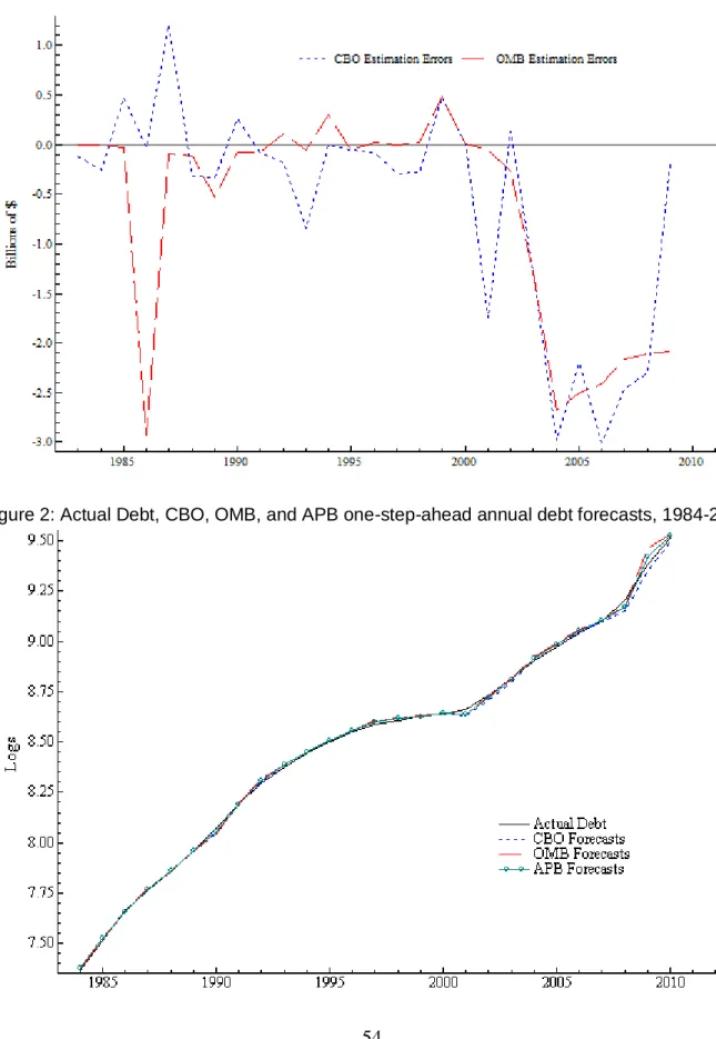
The first series of interest from these sources are the CBO and OMB estimates of the actual value of the debt from the previous year, on which they then base their forecasts.9 Due to data revisions and preliminary data releases, these series sometimes contain errors which are then incorporated into the forecasts. In order to visualize any differences, these estimates are

subtracted from the actual debt for each year to generate the estimation errors for both agencies (Figure 1). Although there have been some differences between the agency estimates and the actual debt, especially from 2004 to 2008, at no point do they ever exceed 1% of the debt and therefore they do not appear to be adding any significant bias.10

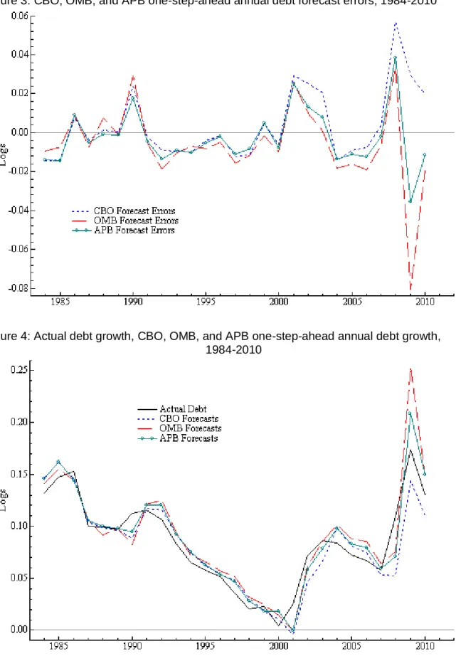
The primary variables of interest are the log levels of the CBO, OMB, and APB one-step-ahead federal debt forecasts in billions of dollars (LCBODF1, LOMBDF1, and LAPBDF1). A first glimpse of how well the forecasts perform is gained by plotting them together with the actual debt (Figure 2). Each forecast is then subtracted from the actual debt in order to generate their forecast errors (Figure 3).11 The largest forecast errors for both agencies were in 1990, 2001, 2002, 2008, and 2009. This is seen more clearly when the actual level of the debt is regressed on each of the forecasts and Impulse Indicator Saturation (IIS) is used with a 1%

9

The Analysis of the President‟s Budget relies on the same estimate that is used in the CBO‟s original forecast. 10

The difference between the estimates and the actual debt do indicate that the encompassing tests have to be performed for both the levels and the growth rate of debt since the results will not be invariant to the transformation. 11

Note that since the forecast is being subtracted from the debt that a value above zero indicates the agency is under predicting the debt while a value below zero indicates that agency is over predicting the debt.

(12)

11

critical value to determine where the structural breaks are in each of the series (Table 3). 12 Using IIS is important because structural breaks in the relationship between debt forecasts and the debt are evidence of problems with the forecasts. Because IIS is a way to detect the presence of structural breaks, it is useful in providing a preliminary assessment of the forecasts. Dummy variables for 1990, 2001, 2002, 2008, and 2009 are found to be significant in at least one of the series (2008 is significant in all three). These dummies also make sense given that during each of these years, the United States was either entering or in the midst of a major recession.13

The growth of the debt and each agency‟s ability to forecast the growth of the debt is also examined (Figure 4). By examining both forecasts of the growth of the debt and forecasts of the debt itself, it can be seen whether the comparisons remain similar for both agencies. For further comparison, the analysis also includes an average of the CBO and OMB forecasts (Average 1) and an average of the OMB and APB forecasts (Average 2). This provides a test of whether a combination of the forecasts could improve upon the individual agency forecasts. For more information on each of the data series used in this paper and their sources see Table 4.

V. ANALYSIS AND RESULTS

The analysis begins with an examination of the CBO and OMB forecasts. Due to the large differences between the forecasts in 2009, the analysis is performed through 2008 and then run again through 2009 and through 2010 to examine how the addition of each year changes the results. Forecasts of both log levels and growth rate are examined because some of the forecast-encompassing tests are not invariant to that transformation. This results from the fact that the growth rate is constructed as a difference between the forecasts and the debt estimates rather than

12

For development and discussions of IIS, see: Hendry and Santos (2005), Hendy, Johansen, and Santos (2008), Johansen and Nielson (2009), and Hendry and Santos (2010). For implementation of IIS in Autometrics/OxMetrics, see: Doornik (2008), and Doornik (2009).

13

For exact recession dates see NBER‟s Business Cycle Expansions and Contractions:

(13)

12

as a difference between the forecasts and the actual value of the debt. After that, each analysis is rerun using Impulse Indicator Saturation (IIS). IIS is used because calculations of the

encompassing test statistics may be affected by outliers or structural breaks. Using IIS helps remove these breaks, which makes calculating the encompassing test statistics more robust. The entire analysis is then performed, using the OMB and APB forecasts. After that, forecast

summary statistics are used to compare all of the forecasts against one another and against several benchmark forecast models. Finally, some possible explanations are offered for why there are large differences between the agency forecasts in recent years and why certain forecasts perform better than others. The following chart summarizes which Tables report which results:

Chart. Categorization of forecast-encompassing results, by table number (table numbers with IIS are in parentheses)

Forecasts Compared OMB vs. CBO OMB vs. APB

Sample end-date 2008 2009 2010 2008 2009 2010

Log levels 5 7 9 17 19 21

(11) (13) (15) (23) (25) (27)

Growth rates 6 8 10 18 20 22

(12) (14) (16) (24) (26) (28)

The forecast encompassing tests for the forecasts of the debt illustrate that through 2008, the OMB forecasts performed better than the CBO forecasts (Table 5). Regardless of how the constant is treated in the equation, the null hypothesis that CBO forecasts encompass OMB forecasts is rejected. This can also be expressed by saying that the CBO‟s forecasts do not encompass the OMB‟s forecasts. On the other hand, the OMB forecasts encompass the CBO forecasts. The average of the OMB and the CBO forecasts also forecast-encompass both the CBO and the OMB forecasts. Given that the null that b1+b2=1 cannot be

rejected, which suggests that the series and their forecasts may be cointegrated, the tests are adapted to account for this property.

(14)

13

agency forecasts individually. The difference between the OMB and the CBO forecasts forecast-encompasses the CBO residuals, regardless of how the constant is treated. On the other hand, the difference between the CBO and the OMB forecasts does not forecast-encompass the OMB residuals. However, the differences between the average and the CBO / OMB forecasts forecast-encompass the CBO / OMB residuals. The results indicate that, while the OMB debt forecasts perform better than the CBO debt forecasts over this sample, averages of the two forecasts outperformed both individual forecasts.

The forecasts of the growth rate of the debt are examined next. The forecast encompassing tests of the growth rate through 2008 have similar findings as the log levels (Table 6). The tests continue to indicate that the CBO forecasts do not forecast-encompass the OMB forecasts, albeit at lower confidence levels. Furthermore, the tests illustrate that the OMB forecast-encompasses the CBO and that the average forecast-encompasses both the CBO and the OMB. The difference between the OMB and the CBO forecast-encompasses the CBO residuals. Furthermore, the difference between the CBO and the OMB does not forecast-encompass the OMB residuals while the difference between the average and the CBO / OMB forecasts,

forecast-encompasses the CBO / OMB residuals. These results reinforce the conclusions that the OMB forecasts encompass and thus performed better than CBO forecasts, while the average of the two agency‟s forecasts encompass both the individual agency forecasts through 2008.

These findings change when the analysis is extended beyond 2008. For forecasts of the actual debt level and growth rate through 2009 (Table 7 and Table 8), the CBO does not forecast-encompass the OMB while the OMB also does not forecast-encompass the CBO. However, the average forecast-encompasses both the OMB and CBO regardless of how the constant is treated. For forecasts of the debt through 2010 (Table 9 and Table 10), the results are

(15)

14

similar in that neither CBO or OMB encompass one another, and the average forecast-encompasses both forecasts individually. Thus, while OMB forecasts of the debt performed better than the CBO forecasts through 2008, neither agency was able to forecast-encompass the other through 2010 (that is, OMB‟s forecast errors increased significantly, while the CBO‟s forecast errors remain fairly constant). At the same time, the average forecast performed better than either forecaster individually throughout all three samples.

The same analysis is rerun for the CBO and OMB forecasts, using IIS to include dummies significant at a 1% critical value. The dummy for 2008 is significant in all of the encompassing tests for all of the samples, which illustrates how large the structural break was that year and how poorly all of the forecasts performed. The results through 2008 (actually 2007 since 2008 is dummied out) are similar to the previous analysis (Table 11 and Table 12), but through 2009 none of the forecasts forecast-encompass one another (Table 13 and Table 14). When the analysis is extended through 2010, once again the average forecast-encompasses the individual forecasts (Table 15 and Table 16). However, for all three time periods there is obvious sensitivity in terms of how the constant is treated, which suggests that once the largest outliers are removed there is a significant amount of bias in the forecasts.

When the encompassing tests are performed for the OMB and the APB forecasts, there are very different results. The forecast encompassing tests for the forecasts of the levels of debt and growth rate illustrate that through 2008, the OMB, APB, and the average of those two forecasts all forecast-encompass one another (Table 17 and Table 18). This results from the fact that the OMB and APB forecasts are highly collinear through 2008. Thus, when either one of them is eliminated, there is no significant change in the effectiveness of explaining the debt.

(16)

15

the results change again. In 2009, the OMB does not forecast-encompass the APB for both the level and the growth rate. On the other hand, the APB forecast-encompasses the OMB (Table 19

and Table 20). At the same time, the average of the APB and OMB forecasts does not forecast-encompass either the APB or the OMB. These results continue to hold when extended through 2010 (Table 21 and Table 22).

Rerunning the OMB and APB analysis using IIS, similar to the OMB and CBO analysis, the dummy for 2008 is found to be significant in every equation for all of the samples. However, the results through 2008 change substantially where the OMB does not forecast-encompass the APB while the APB forecast-encompasses OMB and the average forecast-encompass both OMB and APB (this is especially true for the level of the debt) (Table 23 and Table 24). Through 2009, none of the forecasts forecast-encompass one another, regardless of the test or how the constant is treated (Table 25 and Table 26). The results are similar through 2010, where none of the forecasts are consistently able to forecast-encompass the others14 (Table 27 and Table 28). This suggests that while the APB performs better than the OMB during structural breaks, it does not perform well enough to encompass the structural breaks (or the OMB forecasts when

including structural breaks).

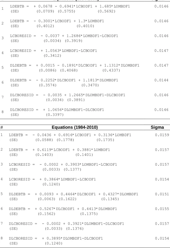
The coefficients in several of the forecast encompassing equations from the analysis highlight these results. From the first part of the analysis, estimates from equations (1) and (2) show that through 2008, the CBO forecasts have coefficients ranging from -0.7 to -0.3 while the OMB forecasts have coefficients ranging from + 1.7 to + 1.3 (Table 29). This suggests that the actual debt was higher than what the CBO forecast, while the OMB over forecast the debt. However, looking at the same equations through 2010, the CBO forecasts have coefficients

14

The exception to this is null hypothesis (c) where it is tested whether agency 2 does not explain agency 1‟s forecast error. The tests often fail to reject this null hypothesis given the similarity of the two forecasts being tested.

(17)

16

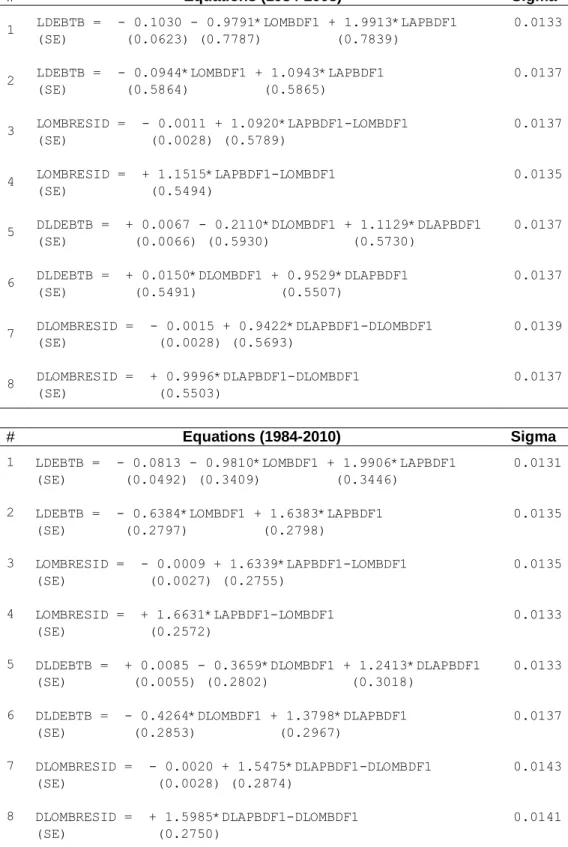
around 0.7 while the OMB forecasts have coefficients around 0.3. From the second part of the analysis, estimates from equations (1) and (2) show that through 2008, the OMB forecasts have coefficients ranging from -1 to -1.1 while the APB forecasts have coefficients ranging from 2 to 1.1, which does not change considerably when extended through 2010 (Table 30). For both parts of the analysis, while the estimated equations through 2010 usually provide a slightly worse explanation of the debt than through 2008 (when looking at the sigma), the fit of the variables, as measured by the standard errors on the coefficients, improves significantly through 2010. This suggests that by extending analysis through 2009 and 2010 a problem of collinearity between the forecasts is reduced.

Additional insight can be gained by numerically comparing the bias, error variance, and the root mean square forecasting errors (RMSFE) for the different forecasts with one another and two benchmark forecasting models (Table 31). Through 2008, 2009 or 2010, each of the

forecasts and their averages perform better than a random walk model or a double differenced device.15 When the analysis is restricted to only the CBO, the OMB, and their average, the OMB forecasts have the smallest error variance and RMSFE through 2008, followed by the average forecasts, while the CBO forecasts have the highest bias, error variance, and RMSFE.16 For the samples through 2009 and also 2010, the average forecasts have the smallest bias, error variance, and RMSFE, followed by the CBO forecasts and then the OMB forecasts. However, when the analysis is extended to include the APB forecasts and the average of the APB and OMB forecasts then the results are different. Regardless of which sample is chosen for the analysis, the APB forecasts outperform all of the other forecasts with the lowest error variance and RMSFE, even though the average of CBO and OMB (Average 1) always has a lower bias. None of these results

15

Hendry (2006) shows that a simple double differenced device can outperform much more complicated models. 16

The average forecast has a bias that is slightly closer to zero than the OMB forecast. In this case negative indicates a tendency to over project the debt while positive indicates a tendency to under project the debt.

(18)

17

change significantly when the growth of the debt is examined.

In general, the average of the CBO and the OMB forecasts is more robust to changes in the economy and as a result is better at forecasting the debt and the change in the debt than the individual agency forecasts. This is supported by Clements and Hendry (2004), who show how pooling forecasts can add value when individual forecasting models are differentially mis-specified. Furthermore, Hendry and Mizon (2005) illustrate that there may be a need to pool across forecasting and policy models when there are structural breaks or policy regime shifts. As a result, individual forecasts‟ weaknesses can be ameliorated by combining them.

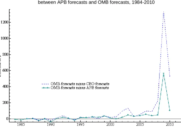
Graphs of the CBO and OMB forecasts clarify their differences. While the two forecasts typically follow one another fairly closely (Figure 5), the largest difference between them occurred in 2009, when they differed by over $1.34 trillion. The difference between the two forecasts occurs because, in 2009, the OMB over-predicted debt by $958 billion whereas the CBO under predicted debt by $381 billion. By contrast, the OMB and APB forecasts for 2009 differ by only $0.57 trillion. Both of the agencies‟ debt forecasts can be dissected into their individual budget components (Table 32). In 2009, the CBO and OMB debt forecasts differed in their forecasts of the deficit ($655 billion) and other expenditures and revenues not included within the budget ($684 billion).

A big reason for the differences in these numbers is due to how and when the forecasts were made. In terms of how they are made, the CBO bases its forecasts on the assumption of current policy whereas the OMB forecasts are based on assumed changes in fiscal policy.17 This important difference means that the CBO has much less flexibility to forecast changes in the debt based on potential policy changes (which during a recession could be very important). It also

17

(19)

18

means that the CBO forecasts are grounded in what has already happened instead of being able to speculate on the effects of proposed policy changes.

When the forecasts are made can also play an important role. While on average the OMB releases its forecasts a week after the CBO, in 2009 the OMB released its forecast on February 26th, which was more than a month after the CBO released theirs (January 8th). In this particular year, in the midst of a financial crisis and a major recession, timing was crucial. On February 17th, the president signed into law a $787 billion stimulus package, which more than accounts for differences in the deficit forecasts for the CBO and the OMB.18 Around the same time, the Treasury Department established several programs to help stabilize the financial system, which account for the differences in the other category. Thus, especially in the midst of structural breaks and regime shifts, the timing of a forecast plays an important role in its forecast performance.

However, how the forecast was generated and when it was released does not account for all of the potential differences between the agencies forecasts. For example, because the OMB releases its forecasts later and takes into account policy changes, it would be expected that that the OMB‟s forecasts would encompass the CBO‟s forecasts. However, there are potentially other factors that reduce the OMB‟s forecast accuracy.19 Thus, by using a combination of the two forecasts the forecasts are robustified against a variety of potential biases, policy changes as well as against forecast mis-specification, thereby improving forecasts of the debt.

VI. CONCLUSION

This paper compares one-step-ahead debt forecasts from the Congressional Budget Office

18_{Meckler, Laura, “Obama Signs Stimulus into Law”, WSJ, Feb. 18, 2009.} 19

Several articles point to OMB‟s strategy of intentionally over predicting the deficit / debt so that it can improve its outlook in later revisions. See for example: OMB Watch, “OMB Mid Session Review Gives Limited Picture of Budget Crisis”, OMB Watch, July 11, 2006.

(20)

19

and the Office of Management and Budget over the past 27 years. Using several summary statistics and forecast encompassing tests, fairly consistent conclusions are reached. First, the agency forecasts all perform better than the benchmark forecasting models. Second, the OMB outperformed the CBO through 2008 but then deteriorated sharply in 2009 and 2010 due to structural breaks and policy shifts. Furthermore, for all three samples the average of the two forecasts performed better than either of them individually. Third, when the APB forecasts are included in the analysis they perform even better than the average or the individual agency forecasts. Finally, all of these results still hold up (albeit more weakly) when the structural breaks in the analysis are accounted for, despite evidence of increased bias.

In conclusion, while both the Congressional Budget Office and the Office of Management and Budget‟s forecasts are relatively successful in forecasting the debt, each agency‟s forecast remains incomplete and could benefit from further information that the other agency takes into account. When only one of the agency‟s forecasts is used, there is an

incomplete and potentially distorted picture of the future levels and changes in government debt. The Analysis of the President‟s Budget helps remedy this problem. It effectively acts as a combination of the two forecasts in that it includes information from both agencies in its

forecasts. While the analysis in this paper did not directly compare the Analysis of the President‟s Budget with the average of the CBO and OMB forecasts, the forecast summary statistics suggest that the APB performs best. However, this improved analysis is released up to several months after the CBO and the OMB forecasts, which reduces its effectiveness for policy making despite the improved information content. Therefore, it is important that both agency forecasts of the debt continue to be taken into consideration to better forecast the future trajectories of the United States‟ gross federal debt.

(21)

20

VII. REFERENCES

Applebaum, Anne (2010). “America‟s debt spiral resembles Greece‟s crisis”. The Washington Post, Feb. 17, 2010.

http://www.washingtonpost.com/wp-dyn/content/article/2010/02/16/AR2010021604549.html (accessed November 30, 2010). Belongia, Michael (1988). Are economic forecasts by government agencies biased? Accurate?

Federal Reserve Bank of St. Louis Review 70, 15-23.

Chong, Yock Y., and David F. Hendry (1986). Econometric Evaluation of Linear Macro- Economic Models. The Review of Economic Studies, 53, no. 4, Econometrics Special Issue (August), 671-690.

Clements, Michael P., and David F. Hendry (1993). On the Limitations of Comparing Mean Square Forecast Errors. Journal of Forecasting, 12, no. 8, 617-637.

______ (2004). Pooling of forecasts. Econometrics Journal, 7, 1-31.

Cohen, Darrel, and Glenn Follette (2003). Forecasting Exogenous Fiscal Variables in the United States. Federal Reserve Board, Finance and Economics Discussion Series, 59.

http://www.federalreserve.gov/pubs/feds/2003/200359/200359abs.html. Corder, Kevin J. (2005). Managing Uncertainty: The Bias and Efficiency of Federal

Macroeconomic Forecasts. Journal of Public Administration Research and Theory, 15, no. 1 (January), 55-70.

Doornik, Jurgen A. (2008). Encompassing and Automatic Model Selection. Oxford Bulletin of

Economics and Statistics, 70, supplement, 915-925.

Doornik, Jurgen A. (2009). Autometrics, Chapter 4 in J. L. Castle and N. Shephard (eds.) The Methodology and Practice of Econometrics: A Festschrift in Honour of David F. Hendry. Oxford University Press, Oxford, 88-121.

Doornik, Jurgen A., and David F. Hendry (2009). Empirical Econometric Modelling using PcGive: Volume I. 6th, London: Timberlake Consultants Press.

Douglas, James W., and George A. Krause (2005). Institutional Design versus Reputational Effects on Bureaucratic Performance: Evidence from U.S. Government Macroeconomic and Fiscal Projections. Journal of Public Administration Research and Theory, 15, no. 2 (April), 281-306.

Engstrom, Erik J., and Samuel Kernell (1999). Serving Competing Principals: The Budget Estimates of OMB and CBO in an Era of Divided Government. Presidential Studies

(22)

21

Ericsson, Neil R. (1992). Parameter Constancy, Mean Square Forecast Errors, and Measuring Forecast Performance: An Exposition, Extensions, and Illustration. Journal of Policy

Modeling 14, no. 4, 465-495.

Ericsson, Neil R. and Jaime Marquez (1993). Encompassing the Forecasts of U.S. Trade Balance Models. The Review of Economics and Statistics, 75, no. 1 (February), 19-31.

Foster, J. D., and James C. Miller III (2000). The Tyranny of Budget Forecasts. The Journal of

Economic Perspectives, 14, no. 3 (Summer), 205-215.

Frendreis, John, and Rayond Tatlovich (2000). Accuracy and Bias in Macroeconomic

Forecasting by the Administration, the CBO, and the Federal Reserve Board. Polity, 32, no. 4 (Summer), 623-632.

Hendry, David F. (2006). Robustifying Forecasts from equilibrium-correction systems. Journal

of Econometrics, 135, 399-426.

Hendry, David F., and Carlos Santos (2005). Regression Models with Data-based Indicator Variables. Oxford Bulletin of Economics and Statistics, 67, Issue 5, 571-595.

Hendry, David F., and Carlos Santos (2010). An Automatic Test of Super Exogeneity, Chapter 12 in M. W. Watson, T. Bollerslev, and J. Russell (eds.) Volatility and Time Series Econometrics: Essays in Honor of Robert F. Engle. Oxford University Press, Oxford, 164-193.

Hendry, David F., and Grayham E. Mizon (2001). Forecasting in the Presence of Structural Breaks and Policy Shifts, In, Andrews, Donald W. and Stock, James H. (eds.) Identification and Inference for Econometric Models: Essays in Honor of Thomas Rothenberg. Cambridge, UK, Cambridge University Press, 480-502.

Hendry, David F., Soren Johansen, and Carlos Santos (2008). Automatic selection of indicators in a fully saturated regression. Computational Statistics, 32, Issue 2, 317-335.

Howard, James A (1987). Government Economic Projections: A Comparison Between CBO and OMB Forecasts. Public Budgeting & Finance, 7, Issue 3, 14-25.

Johansen, Soren, and Bent Nielsen (2009). An Analysis of the Indicator Saturation Estimator as a Robust Regression Estimator, Chapter 1 in J. L. Castle and N. Shephard (eds.) The

Methodology and Practice of Econometrics: A Festschrift in Honour of David F. Hendry. Oxford University Press, Oxford, 1-36.

Kamlet, Mark S., David C. Mowery, and Tsai-Tsu Su (1987). Whom Do You Trust? An

Analysis of Executive and Congressional Economic Forecasts. Journal of Policy Analysis

(23)

22

McNees, Stephen K. (1995). An assessment of the „official‟ economic forecasts. New England

Economic Review (July/August), 13-24.

Meckler, Laura (2009). “Obama Signs Stimulus into Law”. The Wall Street Journal, February 18, 2009. http://online.wsj.com/article/NA_WSJ_PUB:SB123487951033799545.html (accessed August 8, 2010).

OMB Watch (2006). “OMB Mid Session Review Gives Limited Picture of Budget Crisis”. OMB Watch, July 11, 2006. http://www.ombwatch.org/node/2992 (accessed November 30, 2010).

Plesko, George A. (1988). The Accuracy of Government Forecasts and Budget Projections.

National Tax Journal, 41, no. 4 (December), 483-501.

Pozen, Robert (2010). “The US Public debt hits its tipping point”. The Boston Globe, Feb. 23, 2010.

http://www.boston.com/bostonglobe/editorial_opinion/oped/articles/2010/02/23/the_us_p ublic_debt_hits_its_tipping_point/ (accessed November 30, 2010).

U.S. Congressional Budget Office (1983-2010). An Analysis of the President‟s Budgetary Proposals. Washington, DC: Government Printing Office.

http://www.cbo.gov/publications/ bysubject.cfm?cat=0 (accessed August 3, 2010). U.S. Congressional Budget Office (1983-2010). The Economic and Budget Outlook.

Washington, DC: Government Printing Office. http://www.cbo.gov/publications/ bysubject.cfm?cat=0 (accessed June 3, 2010).

______ (2010). CBO‟s Economic Forecasting Record: 2010 Update. www.cbo.gov/doc.cfm?index=11553(accessed July 10, 2010).

U.S Department of Treasury, Financial Management Service (1983-2010). Treasury Bulletin. Washington DC: Government Printing Office: http://www.fms.treas.gov/bulletin (accessed November 30, 2010).

U.S. Executive Office of the President, Office of Management and Budget (1983- 2010). Budget of the United States Government. Washington

DC: Government Printing Office. http://www.gpoaccess.gov/usbudget/browse.html (accessed June 3, 2010).

(24)

23

VIII. TABLES

Table 1. Previous Studies

Study Forecasts Variables Horizon Time Summary of Findings Kamlet, Mowery, and Su (1987) CBO, OMB, NBER, ARIMA

real GNP growth rate, inflation, unemployment

short / long 1976-1984 OMB more biased than CBO (long) Howard (1987) CBO, OMB real GNP growth rate,

GNP deflator, CPI, unemployment, Treasury rates

short 1976-1985 OMB forecasts are biased

Plesko (1988) CBO, OMB nominal GDP, revenues, outlays

short 1974-1988 OMB more biased than CBO

Belongia (1988)

CBO, CEA, Private

real GNP growth rate, GNP deflator,

unemployment

short 1976-1987 Private best, CBO and CEA equally bad McNees (1995) CBO, CEA, FRB, Private inflation, GNP, unemployment

long 1976-1994 CEA more biased than CBO, FOMC, and Private Frendreis and Tatalovich (2000) CBO, OMB, FRB GNP growth, inflation, unemployment

short 1979-1997 CBO best, followed by FRB and then OMB Cohen and Follette (2003) CBO, OMB, FRB

budget short 1977-2003 CBO encompasses

OMB Douglas and

Krause (2005)

CBO, OMB, FRB

real and nominal GDP, inflation, unemployment, revenues, outlays, budget

short 1976-2001 FRB best with unemployment, CBO worst in tax revenues, all else indistinguishable. Corder (2005) CBO, OMB,

SSA

GDP, Inflation,

unemployment, interest rates

short / long 1976-2003 CBO better with GPD, OMB better with

unemployment, neither with interest rates (long)

CBO (2010) CBO, OMB, Private

output, inflation, Treasury rates, long-term interest rates, wage and salary disbursements

short / long 1980-2008 CBO and OMB perform just as good (short and long)

(25)

Table 2. Forecast Release Dates, Debt, and Debt Forecasts

Yeara Release Dates

b

Actual Valued

Forecastsd

CBO OMB APB Diff1c Diff2c CBO OMB APB

1984 2/07 2/01 2/22 6 -21 1,576.75 1,600.00 1,591.57 1,599.00 1985 2/06 2/04 2/27 2 -23 1,827.47 1,853.00 1,841.08 1,854.00 1986 2/18 2/05 2/26 13 -21 2,129.96 2,114.00 2,112.00 2,110.60 1987 1/27 1/05 2/19 22 -45 2,355.21 2,364.00 2,372.40 2,367.20 1988 2/04 2/18 3/04 -14 -15 2,600.68 2,598.00 2,581.60 2,603.00 1989 1/18 1/09 3/09 9 -59 2,865.66 2,865.00 2,868.80 2,869.00 1990 1/24 1/29 3/08 -5 -38 3,206.26 3,131.00 3,113.30 3,150.00 1991 1/23 2/04 3/01 -12 -25 3,598.92 3,606.00 3,617.84 3,616.00 1992 1/22 1/29 3/01 -7 -32 4,002.82 4,039.00 4,077.50 4,058.00 1993 1/26 2/17 3/01 -22 -12 4,351.15 4,392.00 4,396.70 4,391.00 1994 1/27 2/07 4/01 -11 -53 4,644.00 4,690.00 4,676.00 4,692.00 1995 1/25 2/06 4/01 -12 -54 4,920.95 4,942.00 4,961.50 4,947.00 1996 e5/01 2/02 5/01 89 -89 5,181.92 5,191.00 5,207.30 5,193.00 1997 1/28 2/06 3/01 -9 -23 5,369.70 5,436.00 5,453.70 5,431.00 1998 1/28 2/02 3/03 -5 -27 5,478.72 5,540.00 5,543.60 5,524.00 1999 1/29 2/01 3/01 -3 -30 5,606.49 5,579.00 5,614.90 5,578.00 2000 1/26 2/07 3/21 -12 -43 5,629.01 5,665.00 5,686.00 5,674.00 2001 1/31 2/28 5/01 -28 -62 5,770.25 5,603.00 5,625.00 5,627.00 2002 1/23 2/04 3/18 -12 -42 6,198.13 6,043.00 6,137.10 6,117.00 2003 1/30 2/03 3/31 -4 -56 6,758.72 6,620.00 6,752.00 6,706.00 2004 1/27 2/02 2/27 -6 -25 7,352.02 7,459.00 7,486.40 7,453.00 2005 1/25 2/07 3/04 -13 -25 7,902.80 7,975.00 8,031.40 7,991.00 2006 1/26 2/06 3/03 -11 -25 8,448.99 8,515.00 8,611.50 8,556.00 2007 1/25 2/05 3/02 -11 -25 8,948.53 8,915.00 9,007.80 8,968.00 2008 1/23 2/04 3/03 -12 -28 9,983.69 9,432.00 9,654.40 9,606.00 2009 1/08 2/26 3/20 -49 -22 11,873.81 11,529.00 12,867.50 12,303.00 2010 1/27 2/01 3/05 -5 -32 13,526.63 13,260.00 13,786.60 13,684.00 Average Differencef -8 -31 Notes: a

The year that the forecast was released and the year that is being forecast (ending Sept 30th).

b

Month/Day. The release date for the CBO and the APB forecasts is the date they are presented to Congress. The release date for the OMB forecasts is the date of the Presidents message.

c

Difference in days: Calculated for Diff1 by subtracting the OMB release date from the CBO release date. Thus, a negative value means the OMB forecast was released after the CBO forecast whereas a positive value means the OMB forecast was released before the CBO forecast. Calculated for Diff2 by subtracting the APB release date from the OMB release date. Thus, a negative value means the APB forecast was released after the OMB forecast.

d

Billions of $

e

The 1996 forecast for CBO is the revised forecast since the original forecast was not published this year.

f

(26)

25

Table 3. Summary Statistics

The estimation sample is: 1984 - 2010

CBO:

Coefficient Std.Error t-value t-prob Part.R^2 I:2008 0.050 0.015 3.40 0.002 0.325 Constant -0.072 0.043 -1.67 0.108 0.104 LCBODF1 1.009 0.005 198.00 0.000 0.999 sigma 0.014 RSS 0.00462880349 R^2 0.999 F(2,24) = 2.107e+004 [0.000]** Adj.R^2 0.999 log-likelihood 78.751 no. of observations 27 no. of parameters 3 mean(LDEBTB) 8.495 se(LDEBTB) 0.559 AR 1-2 test: F(2,22) = 1.816 [0.186]

ARCH 1-1 test: F(1,25) = 0.231 [0.635] Normality test: Chi^2(2) = 5.134 [0.077] Hetero test: F(2,23) = 0.983 [0.389] Hetero-X test: F(2,23) = 0.983 [0.389] RESET23 test: F(2,22) = 1.750 [0.197]

OMB:

Coefficient Std.Error t-value t-prob Part.R^2 I:1990 0.035 0.007 4.90 0.000 0.545 I:2001 0.035 0.007 5.00 0.000 0.556 I:2002 0.020 0.007 2.87 0.010 0.291 I:2008 0.047 0.007 6.48 0.000 0.677 I:2009 -0.065 0.008 -8.55 0.000 0.785 Constant 0.054 0.023 2.40 0.026 0.224 LOMBDF1 0.993 0.003 370.00 0.000 0.999 sigma 0.007 RSS 0.00094246585 R^2 0.999 F(6,20) = 2.876e+004 [0.000]** Adj.R^2 0.999 log-likelihood 100.237 no. of observations 27 no. of parameters 7 mean(LDEBTB) 8.495 se(LDEBTB) 0.559 AR 1-2 test: F(2,18) = 0.387 [0.684]

ARCH 1-1 test: F(1,25) = 0.525 [0.476] Normality test: Chi^2(2) = 0.999 [0.607] Hetero test: F(2,19) = 0.836 [0.449] Hetero-X test: F(2,19) = 0.836 [0.449] RESET23 test: F(2,18) = 0.721 [0.500]

APB:

Coefficient Std.Error t-value t-prob Part.R^2 I:2001 0.030 0.010 3.15 0.005 0.311 I:2008 0.044 0.010 4.51 0.000 0.480 I:2009 -0.029 0.010 -2.90 0.008 0.276 Constant 0.011 0.030 0.35 0.731 0.006 LAPBDF1 0.998 0.004 278.00 0.000 0.999 sigma 0.009 RSS 0.00189360599 R^2 0.999 F(4,22) = 2.361e+004 [0.000]** Adj.R^2 0.999 log-likelihood 90.8176 no. of observations 27 no. of parameters 5 mean(LDEBTB) 8.495 se(LDEBTB) 0.559 AR 1-2 test: F(2,20) = 1.148 [0.337]

ARCH 1-1 test: F(1,25) = 0.020 [0.888] Normality test: Chi^2(2) = 6.265 [0.044]* Hetero test: F(2,21) = 0.346 [0.711] Hetero-X test: F(2,21) = 0.346 [0.711] RESET23 test: F(2,20) = 1.235 [0.312]

(27)

26

Table 4. Variables

Variable Description Units Periods Sources

LDEBTB Annual value of total gross federal

debt outstanding (held by public and intra-governmental holdings) in logs.

Billions of Dollars 1983-2010 Financial Management Service (FMS)

LCBODF1 Annual one-step-ahead forecast of

Total Gross Federal Debt from the CBO in logs. Billions of Dollars 1984-2010 Congressional Budget Office

LOMBDF1 Annual one-step-ahead forecast of

Total Gross Federal Debt from the OMB in logs. Billions of Dollars 1984-2010 Office of Management and Budget

LAPBDF1 Annual one-step-ahead forecast of

Total Gross Federal Debt from the Analysis of the President’s Budget in logs. Billions of Dollars 1984-2010 Congressional Budget Office

LCBORESID Annual value of total gross federal

debt minus the one-step-ahead forecast of the debt from the CBO in logs. Billions of Dollars 1984-2010 FMS and CBO

LOMBRESID Annual value of total gross federal

debt minus the one-step-ahead forecast of the debt from the OMB in logs. Billions of Dollars 1984-2010 FMS and OMB

LAPBRESID Annual value of total gross federal

debt minus the one-step-ahead forecast of the debt from the Analysis of the President’s Budget in logs.

Billions of Dollars

1984-2010

FMS and CBO

DLDEBTB Annual difference of the annual value

of total gross federal debt in logs.

Billions of Dollars 1984-2010 Financial Management Service

DLCBODF1 Annual difference between the

one-step-ahead CBO forecast of the debt and the CBO estimate of the debt for the previous year.

Billions of Dollars 1984-2010 Congressional Budget Office

DLOMBDF1 Annual difference between the

one-step-ahead OMB forecast of the debt and the OMB estimate of the debt for the previous year in logs

Billions of Dollars 1984-2010 Office of Management and Budget

DLAPBDF1 Annual difference between the

one-step-ahead APB forecast of the debt and the CBO estimate of the debt for the previous year.

CBODE Annual estimate of the total gross

federal debt outstanding by the Congressional budget office

OMBDE Annual estimate of the total gross

federal debt outstanding by the Office of Management and Budget

Billions of Dollars 1983-2009 Office of Management and Budget

(28)

27

Table 5. Forecast-Encompassing Test Statistics for Alternative US Federal Debt Forecasts One-step-ahead (Log levels, 1984-2008)

Encompassing Forecast (Encompassed Forecast)

Treatment of constant term (f)

Null Hypotheses (a)-(e)

b1 = 1,

b2 = 0 b2=0

b1≡1,

b2=0 b1+b2=1 b3=0

CBO (OMB) b0 unrestricted 5.752** 8.768** 2.128 1.019 10.476**

[0.010] [0.007] [0.158] [0.324] [0.004] (2,22) (1,22) (1,23) (1,22) (1,23) b0 = 0 3.956* 5.690* 1.201 1.102 5.420* [0.021] [0.010] [0.319] [0.350] [0.012] (3,22) (2,22) (2,23) (2,22) (2,23) b0 ≡ 0 5.497* 10.503** 0.354 1.293 9.583** [0.011] [0.004] [0.557] [0.267] [0.005] (2,23) (1,23) (1,24) (1,23) (1,24)

OMB (CBO) b0 unrestricted 0.744 1.455 0.038 1.019 0.470

[0.487] [0.241] [0.847] [0.324] [0.50] (2,22) (1,22) (1,23) (1,22) (1,23) b0 = 0 0.744 0.736 0.383 1.102 0.606 [0.537] [0.490] [0.686] [0.350] [0.554] (3,22) (2,22) (2,23) (2,22) (2,23) b0 ≡ 0 0.660 0.559 0.777 1.293 0.027 [0.526] [0.462] [0.387] [0.267] [0.870] (2,23) (1,23) (1,24) (1,23) (1,24)

AVE1 (CBO) b0 unrestricted 2.434 4.321* 0.463 1.019 3.845

[0.111] [0.050] [0.503] [0.324] [0.062] (2,22) (1,22) (1,23) (1,22) (1,23) b0 = 0 1.628 2.438 0.239 1.102 1.931 [0.212] [0.111] [0.789] [0.350] [0.168] (3,22) (2,22) (2,23) (2,22) (2,23) b0 ≡ 0 1.992 3.976 0.007 1.293 2.658 [0.159] [0.058] [0.936] [0.267] [0.116] (2,23) (1,23) (1,24) (1,23) (1,24)

AVE1 (OMB) b0 unrestricted 2.434 4.321* 0.491 1.019 3.845

[0.111] [0.050] [0.490] [0.324] [0.062] (2,22) (1,22) (1,23) (1,22) (1,23) b0 = 0 1.628 2.438 0.253 1.102 1.931 [0.212] [0.111] [0.779] [0.350] [0.168] (3,22) (2,22) (2,23) (2,22) (2,23) b0 ≡ 0 1.992 3.976 0.006 1.293 2.658 [0.159] [0.058] [0.937] [0.267] [0.116] (2,23) (1,23) (1,24) (1,23) (1,24) Notes:

1. The three entries within a given block of numbers in the last five columns are: the approximate F statistic for testing the null hypothesis, the tail probability associated with that value of the F statistic (in square brackets), and the degrees of freedom for the F statistic (in parentheses).

2. The regressions for Null Hypothesis tests come from (a) Chong and Hendry (1986), (b) Chong and Hendry (1986), (c) Chong and Hendry (1986), (d) Ericsson (1993), (e) Ericsson (1992), and (f) Ericsson and Marquez (1993).

3. AVE1 is the average of the CBO and the OMB forecasts.

4. b3 is where b2-b1 is constrained to equal b3 and where b1 is also constrained to equal unity.

(29)

28

Table 6. Forecast-Encompassing Test Statistics for Alternative US Federal Debt Forecasts One-step-ahead (Growth rates, 1984-2008)

b1 = 1,

b2 = 0 b2=0

b1≡1,

b2=0 b1+b2=1 b3=0

CBO (OMB) b0 unrestricted 5.464* 6.802* 1.793 0.545 10.592**

[0.012] [0.016] [0.194] [0.468] [0.004] (2,22) (1,22) (1,23) (1,22) (1,23) b0 = 0 3.771* 5.573* 1.042 0.814 5.493* [0.025] [0.011] [0.369] [0.456] [0.011] (3,22) (2,22) (2,23) (2,22) (2,23) b0 ≡ 0 5.882** 11.588** 0.008 1.657 9.838** [0.009] [0.002] [0.932] [0.211] [0.005] (2,23) (1,23) (1,24) (1,23) (1,24)

OMB (CBO) b0 unrestricted 0.502 0.216 0.950 0.545 0.469

[0.612] [0.647] [0.340] [0.468] [0.50] (2,22) (1,22) (1,23) (1,22) (1,23) b0 = 0 0.555 0.210 0.819 0.814 0.571 [0.650] [0.812] [0.453] [0.456] [0.573] (3,22) (2,22) (2,23) (2,22) (2,23) b0 ≡ 0 0.848 0.397 1.466 1.657 0.037 [0.441] [0.535] [0.238] [0.211] [0.849] (2,23) (1,23) (1,24) (1,23) (1,24)

AVE1 (CBO) b0 unrestricted 2.174 2.487 2.127 0.545 3.880

[0.138] [0.129] [0.158] [0.468] [0.061] (2,22) (1,22) (1,23) (1,22) (1,23) b0 = 0 1.452 1.935 1.068 0.814 1.944 [0.255] [0.168] [0.360] [0.456] [0.166] (3,22) (2,22) (2,23) (2,22) (2,23) b0 ≡ 0 2.252 3.995 0.581 1.657 2.772 [0.128] [0.058] [0.454] [0.211] [0.109] (2,23) (1,23) (1,24) (1,23) (1,24)

AVE1 (OMB) b0 unrestricted 2.174 2.487 1.366 0.545 3.880

[0.138] [0.129] [0.254] [0.468] [0.061] (2,22) (1,22) (1,23) (1,22) (1,23) b0 = 0 1.452 1.935 0.687 0.814 1.944 [0.255] [0.168] [0.513] [0.456] [0.166] (3,22) (2,22) (2,23) (2,22) (2,23) b0 ≡ 0 2.252 3.995 0.342 1.657 2.772 [0.128] [0.058] [0.564] [0.211] [0.109] (2,23) (1,23) (1,24) (1,23) (1,24) Notes: See Table 5.

(30)

29

b1 = 1,

b2 = 0 b2=0

b1≡1,

b2=0 b1+b2=1 b3=0

CBO (OMB) b0 unrestricted 3.514* 3.092 3.872 0.437 6.748*

[0.047] [0.092] [0.061] [0.515] [0.016] (2,23) (1,23) (1,24) (1,23) (1,24) b0 = 0 2.607 3.401 2.304 0.223 3.780* [0.076] [0.051] [0.122] [0.802] [0.037] (3,23) (2,23) (2,24) (2,23) (2,24) b0 ≡ 0 3.777* 6.510* 0.866 0.003 7.863** [0.038] [0.018] [0.361] [0.954] [0.010] (2,24) (1,24) (1,25) (1,24) (1,25)

OMB (CBO) b0 unrestricted 9.160** 14.526** 2.084 0.437 18.312**

[0.001] [0.001] [0.162] [0.515] [0.000] (2,23) (1,23) (1,24) (1,23) (1,24) b0 = 0 7.110** 8.949** 1.992 0.223 10.697** [0.002] [0.001] [0.158] [0.802] [0.001] (3,23) (2,23) (2,24) (2,23) (2,24) b0 ≡ 0 10.692** 17.870** 2.073 0.003 22.268** [0.001] [0.000] [0.162] [0.954] [0.000] (2,24) (1,24) (1,25) (1,24) (1,25)

[0.577] [0.30] [0.934] [0.515] [0.409] (2,23) (1,23) (1,24) (1,23) (1,24) b0 = 0 0.435 0.566 0.092 0.223 0.445 [0.730] [0.576] [0.912] [0.802] [0.646] (3,23) (2,23) (2,24) (2,23) (2,24) b0 ≡ 0 0.442 0.705 0.180 0.003 0.917 [0.648] [0.409] [0.675] [0.954] [0.347] (2,24) (1,24) (1,25) (1,24) (1,25)

(31)

30

b1 = 1,

b2 = 0 b2=0

b1≡1,

b2=0 b1+b2=1 b3=0

CBO (OMB) b0 unrestricted 5.219* 8.687** 0.002 3.018 6.844*

[0.014] [0.007] [0.966] [0.096] [0.015] (2,23) (1,23) (1,24) (1,23) (1,24) b0 = 0 3.789* 5.657* 0.334 1.512 3.850* [0.024] [0.010] [0.719] [0.242] [0.035] (3,23) (2,23) (2,24) (2,23) (2,24) b0 ≡ 0 4.403* 8.757** 0.552 0.843 8.014** [0.024] [0.007] [0.465] [0.368] [0.009] (2,24) (1,24) (1,25) (1,24) (1,25)

OMB (CBO) b0 unrestricted 11.394** 7.584* 3.337 3.018 18.237**

[0.000] [0.011] [0.080] [0.096] [0.000] (2,23) (1,23) (1,24) (1,23) (1,24) b0 = 0 8.661** 6.908** 2.622 1.512 10.592** [0.001] [0.005] [0.093] [0.242] [0.001] (3,23) (2,23) (2,24) (2,23) (2,24) b0 ≡ 0 11.380** 11.146** 4.330* 0.843 22.056** [0.000] [0.003] [0.048] [0.368] [0.000] (2,24) (1,24) (1,25) (1,24) (1,25)

[0.175] [0.883] [0.074] [0.096] [0.416] (2,23) (1,23) (1,24) (1,23) (1,24) b0 = 0 1.310 1.144 1.834 1.512 0.420 [0.295] [0.336] [0.182] [0.242] [0.662] (3,23) (2,23) (2,24) (2,23) (2,24) b0 ≡ 0 0.854 0.139 1.490 0.843 0.870 [0.438] [0.712] [0.234] [0.368] [0.360] (2,24) (1,24) (1,25) (1,24) (1,25)

(32)

31

b1 = 1,

b2 = 0 b2=0

b1≡1,

b2=0 b1+b2=1 b3=0

CBO (OMB) b0 unrestricted 4.213* 3.268 5.013* 0.545 8.027**

[0.027] [0.083] [0.034] [0.468] [0.009] (2,24) (1,24) (1,25) (1,24) (1,25) b0 = 0 3.237* 4.041* 3.102 0.275 4.668* [0.040] [0.031] [0.063] [0.762] [0.019] (3,24) (2,24) (2,25) (2,24) (2,25) b0 ≡ 0 4.665* 7.672* 1.335 0.001 9.703** [0.019] [0.010] [0.258] [0.977] [0.004] (2,25) (1,25) (1,26) (1,25) (1,26)

OMB (CBO) b0 unrestricted 9.891** 15.130** 2.605 0.545 19.594**

[0.001] [0.001] [0.119] [0.468] [0.000] (2,24) (1,24) (1,25) (1,24) (1,25) b0 = 0 7.887** 9.613** 2.526 0.275 11.773** [0.001] [0.001] [0.10] [0.762] [0.000] (3,24) (2,24) (2,25) (2,24) (2,25) b0 ≡ 0 11.769** 19.021** 2.637 0.001 24.477** [0.000] [0.000] [0.116] [0.977] [0.000] (2,25) (1,25) (1,26) (1,25) (1,26)

[0.565] [0.293] [0.906] [0.468] [0.433] (2,24) (1,24) (1,25) (1,24) (1,25) b0 = 0 0.448 0.587 0.094 0.275 0.406 [0.721] [0.564] [0.911] [0.762] [0.670] (3,24) (2,24) (2,25) (2,24) (2,25) b0 ≡ 0 0.404 0.637 0.173 0.001 0.840 [0.672] [0.432] [0.681] [0.977] [0.368] (2,25) (1,25) (1,26) (1,25) (1,26)

(33)

32

b1 = 1,

b2 = 0 b2=0

b1≡1,

b2=0 b1+b2=1 b3=0

CBO (OMB) b0 unrestricted 5.868** 10.343** 0.063 2.973 8.123**

[0.008] [0.004] [0.803] [0.098] [0.009] (2,24) (1,24) (1,25) (1,24) (1,25) b0 = 0 4.404* 6.464** 0.549 1.488 4.745* [0.013] [0.006] [0.585] [0.246] [0.018] (3,24) (2,24) (2,25) (2,24) (2,25) b0 ≡ 0 5.288* 10.305** 1.057 0.790 9.865** [0.012] [0.004] [0.313] [0.383] [0.004] (2,25) (1,25) (1,26) (1,25) (1,26)

OMB (CBO) b0 unrestricted 12.015** 7.573* 3.737 2.973 19.517**

[0.000] [0.011] [0.065] [0.098] [0.000] (2,24) (1,24) (1,25) (1,24) (1,25) b0 = 0 9.373** 7.026** 3.092 1.488 11.653** [0.000] [0.004] [0.063] [0.246] [0.000] (3,24) (2,24) (2,25) (2,24) (2,25) b0 ≡ 0 12.414** 11.379** 5.201* 0.790 24.234** [0.000] [0.002] [0.031] [0.383] [0.000] (2,25) (1,25) (1,26) (1,25) (1,26)

[0.184] [0.963] [0.074] [0.098] [0.441] (2,24) (1,24) (1,25) (1,24) (1,25) b0 = 0 1.266 1.120 1.829 1.488 0.383 [0.308] [0.343] [0.181] [0.246] [0.686] (3,24) (2,24) (2,25) (2,24) (2,25) b0 ≡ 0 0.789 0.086 1.440 0.790 0.794 [0.466] [0.772] [0.241] [0.383] [0.381] (2,25) (1,25) (1,26) (1,25) (1,26)