Benchmarking Cloud-based Data Management Systems

(1)

Benchmarking Cloud-based Data Management Systems

Yingjie Shi, Xiaofeng Meng, Jing Zhao, Xiangmei Hu, Bingbing Liu and Haiping Wang

School of Information, Renmin University of China Beijing, China, 100872

[email protected],

{xfmeng,zhaoj,hxm2008,liubingbing,wanghaiping1022}@ruc.edu.cn

ABSTRACT

Cloud-based data management system is emerging as a scal-able, fault tolerant and efficient solution to large scale data management. More and more companies are moving their data management applications from expensive, high-end ser-vers to the cloud which is composed of cheaper, commodity machines. The implementations of existing cloud-based data management systems represent a wide range of approaches, including storage architectures, data models, tradeoffs in consistency and availability, etc. Several benchmarks have been proposed to evaluate the performance. However, there were no reported studies about these benchmark results which provide users with insights on the impacts of different im-plementation approaches on the performance. We conducted comprehensive experiments on several representative cloud-based data management systems to explore relative perfor-mance of different implementation approaches, the results are valuable for further research and development of cloud-based data management systems.

Categories and Subject Descriptors

H.3.4 [Information Storage and Retrieval]: Systems and Software—Performance evaluation

General Terms

Measurement,Performance

Keywords

cloud, data management, benchmark

1. INTRODUCTION

Cloud computing has emerged as a prevalent infrastruc-ture and attracted a lot of attention of companies and aca-demic circles. Though there has not been a standard deﬁni-tion about cloud computing, we can summarize the substan-tial features of it: scalability, fault tolerance, high perfor-mance cost, pay-as-you-go, etc. Data management system is

Permission to make digital or hard copies of all or part of this work for personal or classroom use is granted without fee provided that copies are not made or distributed for profit or commercial advantage and that copies bear this notice and the full citation on the first page. To copy otherwise, to republish, to post on servers or to redistribute to lists, requires prior specific permission and/or a fee.

one of the applications that are deployed in the cloud, many cloud-based data management systems have been proposed and are serving online right now: BigTable[1] in Google, Cassandra[2] and Hive[3] in Facebook, HBase[4]in Streamy, PNUTS[6] in Yahoo! and many other systems. In order to merge with the cloud computing platform, the data man-agement system should have high availability and fault tol-erance, flexible scalability, and the ability to run in the het-erogeneous environment. Developers of the existing systems choose different solutions to make their data management systems work well in the cloud depending on their different application scenarios.

The developers of many companies are wondering whether their data management applications can be moved to the cloud to get better performance with less cost. However, the application environments and implementation approaches of existing cloud-based data management systems are so var-ious that it is difficult for developers to determine which system is more suitable for their applications. The sig-nificance of conducting comprehensive experiments on the cloud-based data management systems can be summarized as follows: showing the performance advantage of different systems and providing the users with impacts of different technical issues on the performance. The test results and analysis are useful for both further research and develop-ment of cloud-based data managedevelop-ment systems.

There have been several benchmarks proposed to evaluate the performance of cloud-based data management systems, including performance evaluation of the Google’s BigTable [1] which is for systems that do not support structured query language, the performance comparison of Hadoop[15] and some parallel DBMSs [8] which put emphasis on structured query of the systems, and the Yahoo! Cloud Serving Bench-mark(YCSB)[9] framework which supplies several workloads with diﬀerent combinations of insert, read, update and scan. Several experiment reports depending on these benchmarks can also be found, however, all of them focus on one or two systems’ performance evaluation without comparison anal-ysis depending on their implementation approaches. Three cloud-based management systems are included in[9]: Cas-sandra, HBase and PNUTS, they present results of three workloads: update heavy, read heavy and short ranges. And all the workloads in YCSB focus on serving systems just like PNUTS, which provide online read or write access to data. The analytical systems are not included in their workload. And all the systems in their experiment do not use repli-cation, which is widely used in the cloud-based systems for data availability, so they do not evaluate the fault tolerance

(2)

or availability of these systems either. We conduct compre-hensive experiments on the representative cloud-based data management systems, which cover the different approaches on storage architectures and data models. Our workloads and tasks originate from benchmarks in [1] and [8], we make some extensions to investigate the factors that affect perfor-mance of different implementations.

The rest of this article is organized as follows. Section 2 summarizes the existing cloud-based data management sys-tems with emphasis on storage architecture and data model. Section 3 describes the workloads and tasks in the bench-mark. The test results and analysis are given in Section 4. We describe the future work and conclude the article in Section 5.

2. AN OVERVIEW OF EXISTING

CLOUD-BASED DATA MANAGEMENT SYSTEMS

Cloud-based data management system will not replace the traditional RDBMS in the near future, however, it sup-plies another choice for the applications which are suitable to be deployed in the cloud: large scale data analysis and data management in the web applications. Different from transactional applications, data involved in the analysis are rarely updated, so ACID guarantees in the transactional ap-plications are not needed. Data analysis apap-plications are often deployed on shared-nothing parallel databases, but with the increase of data scale, systems will have to scale vertically which costs a lot of money and time to get bet-ter performance. Cloud-based data management systems provide a flexible and economical solution to scale horizon-tally with commodities, and the scaling server resources are transparent to the applications. In the web data manage-ment applications, response time is one of the most im-portant requests except for scalability and fault tolerance. Big data is produced during the interaction between cus-tomers and the sites, and we can not see the increase end in sight. Many companies which supply social network ser-vices have moved some of their applications to cloud-based data management systems because of data explosion[13]. During the existing cloud-based data mangement systems, BigTable, HBase, HyperTable, Hive and HadoopDB[10] are mostly used for analytical data management applications, while PNUTS and Cassandra are used for web data man-agement. Different applications originate from different im-plementation approaches, next we will compare the technical issues from storage architecture and data model.

2.1 Storage Architecture

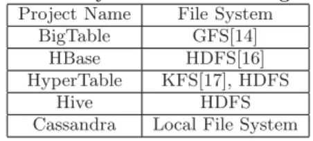
Depending on the persistency design, we can classify the cloud-based data management systems into two kinds: File System-based systems and DBMS-based systems. BigTable, HBase, HyperTable, Hive and Cassandra are File System-based softwares. HBase and HyperTable are open-source im-plementations of BigTable’s architecture, they are called the BigTable-like systems. The BigTable-like systems and Hive all store data in distributed file systems, which is master-slave organized. While Cassandra uses file system directly as the storage layer, which is peer-to-peer organized. Table 1 shows the different file systems they use.

SQL Azure, PNUTS, HadoopDB and Voldemort use tra-ditional DBMS as the storage layer. DBMS’s inherent fea-tures such as query optimization, index techniques can be

Table 1: File Systems in the Storage Layer

Project Name File System BigTable GFS[14]

HBase HDFS[16] HyperTable KFS[17], HDFS

Hive HDFS

Cassandra Local File System

directly utilized in this kind of systems, and it’s easy for this kind of system to support SQL to the users. However, under this kind of architecture, DBMS layer can be a bottleneck for data storage, because all the data storage optimization can only be executed on top of DBMS.

Generally speaking, FileSystem-based systems inherit sev-eral merits from MapReduce[7] if they use MapReduce as the framework, such as scalability, fault-tollerance, adapt-ing to heterogeneous environment, etc. However, most of these systems can not support SQL, except for Hive which can support part of SQL called HQL. DBMS-based systems can support SQL, however, there is a lot of work to do on scalability, fault tolerance, and support for semi-structured and unstructured data.

2.2 Data Model

The data models of existing cloud-based data manage-ment systems are extremely diﬀerent, we classify them into two kinds: the key-value data model and the simpliﬁed re-lational data model.

The key-value data model is a sparse, distributed, persis-tent multidimensional sorted map[1], it is simple and flex-ible. There are no different data types, all data is stored as bytes. The elements in the multidimensional map are not only rows and columns, but also column families, times-tamps, etc. The rows and columns represent what they mean in the relational data model, but the rows are sparse: each row can have different number of columns in one table, and columns can be added during the process of data load-ing. The unique row key identify one record, it is mapped to a list of column families. The column family is mapped to a list of columns, while the column is mapped to a list of times-tamps, then the timestamp is mapped to the value. The value is fixed by a key consisting of row key, column family, column name and timestamp, we can simply summarize the map relationship as<row key,<column family,<columname ,<timestamp, value>>>>. A set of columns are put to-gether into one column family, which is also the data access unit. Data of the same column family is stored in one file on disk, so clients are suggested to put the columns which are often queried together into one column family to get better performance. Timestamps are used in two ways: indexing multiple versions of data, and conflict resolution.

Data in the DBMS-based systems is eventually stored in the RDBMS, they adopt the relational data model with some varieties in order to support distributed applications. For example, traditional relational data model ensures entity in-tegrity and referential inin-tegrity, however, now most cloud-based data management systems do not ensure referential integrity. Hive is one of the systems that use the relational data model, data in Hive is organized into tables which are analogous to tables in relation databases, each table has a

(3)

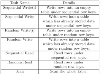
Table 2: Tasks in data read and write benchmark

Task Name Details

Sequential Write(i) Write rows into an empty table under sequential row keys. Sequential Write Write rows into a table

which has already stored data under sequential row keys. Random Write(i) Write rows into an empty table under random row keys. Random Write Write rows into a table

which has already stored data under random row keys. Sequential Read Read rows under

sequential row keys. Random Read Read rows under

random row keys. Scan Scan the whole table.

corresponding HDFS directory[3]. Hive does not support primary key or foreign key yet.

The relational data model has solid theoretical basis and reﬁned implement technologies, however, it is diﬃcult to use it directly in the cloud environment. The key-value data model is simple and easy to implement, however, all sys-tems of this data model support APIs instead of a uniform language like SQL, which supplies sophisticated DDL and DML operations. So there is a lot of work to do to widen the appliation scope of the key-value model systems.

3. WORKLOADS OF THE BENCHMARK

We conducted two benchmarks on several existing cloud-based management systems: data read and write benchmark and structured query benchmark. During the data read and write benchmark, seven tasks are deﬁned to evaluate the read and write performance during diﬀerent situations. The structured query benchmark focus on some basic opera-tions in the structured query language, including key words matching, range query, aggregation and so on. In fact many cloud-based data management systems do not support SQL, we evaluate their performance in this benchmark by coding the client through the APIs they provide. Next we will de-scribe the details of workloads in these two benchmarks.

3.1 Data Read and Write Benchmark

The principles of this benchmark originate from the per-formance evaluation section of BigTable paper[1], we also add some tasks included in a test report[11] which shows the test results of HBase-0.20.0 on 5 servers. There are seven tasks as Table 2 shows.

All of the tasks operate on a column family with one col-umn, one row is written or read during one operation. The row size is 1010 bytes: 1000 bytes for value, and 10 bytes for row key. We write a string of 1000 bytes into one row as the value, each string is composed by characters random gen-erated. The sequential read and write are operations with row keys in order, while random operations using row keys out-of-order, and the motivation is to determine whether performance can be aﬀected by diﬀerent row key choosing methods. Initial write is an operation against an empty ta-ble, while the other kind of write is operation against a table which has already stored data partitioned in the whole

sys-tem. The motivation is to examine how the existing data can affect the write performance of systems with different stor-age architectures. Scan is also reading rows under sequential row keys, the difference between scan and sequential read is that we call the special interfaces the systems supply. Dur-ing the task of sequential read, one row is returned once we call the API, but during the task of scan, all the rows in the table are returned once we call the scan API. Scan is one of the most important applications in the cloud-based data management systems during data analysis. The replication factors of all systems involved are set to 3, which is widely used in the distributed systems.

In addition to the data read and write performance, scal-ability is also an important characteristic of the cloud-based systems. A system has scalability means that more servers will create more capacity and the scaling server resources are transparent to the applications. Speedup is widely used to measure the scalability of distributed systems. In order to evaluate the scalability of systems in a more detailed way, we also compute the speedup during this benchmark by exe-cuting these tasks on systems deployed on diﬀerent numbers of servers.

3.2 Data Load and Structured Query

Bench-mark

Structured query language is widely supported by tradi-tional data management systems, and it makes applications development on the cloud system much easier. Until now, the DBMS-based systems can support part of SQL, while most of the FileSystem-based systems don’t provide SQL APIs. We conduct this benchmark on these two kinds of systems, and for systems that do not support SQL, we imple-mented the structured query through coding on other APIs they provide to analyze their performances. The workload of this benchmark originates from Pavlo’s work[8], it is used to evaluate performance of cloud-based data management systems and parallel databases, focusing on structured data load and query. Our motivation of conducting this bench-mark is to compare the performances of cloud-based data management systems with diﬀerent architectures and imple-mentation approaches on structured data query. Three ta-bles are involved in the dataset, Table 3 described the struc-tures of them. The table of rankings and uservisits simulate the the page ranks and visit logs of web pages. There are ﬁve tasks in this benchmark: data load, grep query, range query, aggregation and fault tolerance.

• Data Load: Data is loaded into cloud-based data man-agement systems from ﬁles on local ﬁle system of the client, the replication factor of data is also set to 3.

• Grep Query: The table of grep contains a column of 10 bytes as the key, and a column of 90 bytes as the ﬁeld to be patterned with some key words, during our test we use the key word ’XYZ’.

• Range Query: Table involved in this task is ”rankings”, which stores information of page URL and page rank. The range query will return the records with page rank in a special region.

• Aggregation: Compute the total adRevenue generated from each sourceIP in the table ”uservisits”, grouped by the column of ”soureIP”.

(4)

Table 3: Tables in the dataset

Table Name Table Structure

grep key VARCHAR(10), ﬁeld ARCHAR(90)

rankings pageRank INT, pageURL VARCHAR(100),avgDuration INT uservisits sourceIP VARCHAR(16), destURL VARCHAR(100),

visitDate DATE, adRevenue FLOAT, userAgent VARCHAR(64), countryCode VARCHAR(3), languageCode VARCHAR(6), searchWord VARCHAR(32), duration INT

Table 4: Testbed Setup

CPU Quad Core 2.33GHz(5 servers) Quad Core 2.66GHz(15 servers) RAM 7GB(5 servers)

8GB(15 servers) Disk 1.8TB(5 servers) 2TB(15 servers) Operating System Linux: Ubuntu 9.04 Server

Network 1000Mbps

The tasks above are basic operations in structured query, most cloud-based data management systems can’t support sophisticated queries currently, however, we can overview their performances in structured query from these simple operations. In a cloud-based data management system with high fault tolerance, a query does not have to be restarted when one of the servers involved in the query failed. We also evaluate the fault tolerance of the systems in this benchmark through comparing the elapsed time during the normal sit-uation and fault sitsit-uation.

4. PERFORMANCE EVALUATION

In this section we describe the implementation details of the benchmark and the analysis of test results. Four systems are focused in the benchmark: HBase, Cassandra, Hive and HadoopDB. We tried to evaluate systems that can cover all the architecture types from open source software: HBase is one of the BigTable-like systems based on master-slave archi-tecture; Cassandra is also Filesystem-based and adopts the P2P architecture; during all the FileSystem-based systems we have surveyed, only HIVE can support SQL; HadoopDB is one of the systems that are based on DBMS. We tune each system to get the best performance in our platform, and every task is executed three times to compute the av-erage result. We choose the latest versions of these systems when we conduct the benchmark: HBase 0.20.3, Cassandra 0.6.0-beta3, Hive 0.6.0. All the cloud-based data manage-ment systems are under active developmanage-ment, so our results can reﬂect the current situations, and the results maybe dif-ferent in the later versions of systems. All of the systems are deployed on 20 servers in our testbed, and the setup of these servers is shown in Table 4.

4.1 Data Read and Write Benchmark

HBase and Cassandra are involved in this benchmark, both of them are FileSystem-based, and neither of them can support SQL. The diﬀerence of these two systems is the architecture: HBase is Master-Slave organized, and Cassan-dra is P2P organized. 5,242,880 rows are involved in every task of this benchmark, and as mentioned in Section 3.1, the row size is 1010 bytes, so the data size of this benchmark is

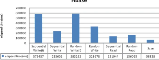
Sequential Write(i) Sequential Write Random Write(i) Random Write Sequential Read Random Read Scan elapsed time(ms) 579457 235601 583292 328678 131944 156055 58828 0 100000 200000 300000 400000 500000 600000 700000 el ap se d ti me( ms ) HBase

Figure 1: HBase performance on 20 nodes

about 5G. The implementation details of this benchmark on these two systems are as follows:

HBase: We adopt the performance evaluation package in

HBase 0.20.3 and modiﬁed some code. All the tasks are im-plemented through MapReduce framework.

Cassandra:We code the evaluation client through the

ba-sic data read and write APIs Cassandra provides. There is no MapReduce interface in Cassandra, we use multithreads in the client to increase the parallelism degree. The client servers are also servers in Cassandra.

4.1.1 Test Results of HBase

Figure 1 illustrates the test results of HBase on 20 nodes(1 master and 19 slaves). The horizontal-axis represents the task type, and the vertical-axis shows the elapsed time. We can find that read speed is faster than that of write, this is very different from the test results of BigTable[1], in which random write is 7 times faster than random read, while se-quential write is 12 times faster than sequential read. Ini-tial writes are slower than writes against an existing table. At first of the initial write, there are just two or three servers working in the task, and as time goes, more and more nodes are involved. But for the writing against an existing table which has already been distributed on 20 servers, there are 20 servers working at the beginning. For the writing against an existing table, tasks are easily to be splitted into the whole system, but for initial write, tasks are splitted among the servers as data is inserted into the servers. So the par-allelism degree of writes against an existing table is bigger than that of the initial write. Scan performs better than both sequential read and random read. Scan is reading rows sequentially, and different from sequential read task which gets one row at once, it can read many rows together each time, so it costs less RPCs than sequential read.

We conduct these seven tasks on 5 slaves, 10 slaves, 15 slaves and 19 slaves separately, Figure 2(a) illustrates the scalability results of HBase, the horizontal-axis represents the number of slaves in the system, and the vertical-axis represents how many rows are operated per second of each task. We can see the performance gets better as the number of nodes increases, although the acceleration is not linear.

(5)

0 20000 40000 60000 80000 100000 120000 5 10 15 19 ro w s/s Sequential Write(i) Sequential Write Random Write(i) Random Write Sequential Read Random Read Scan

(a) The scalability of HBase

0 20 40 60 80 100 0 1 2 3 4 5 5 10 15 19 sp eed u p Sequential Write(i) Sequential Write Random Write(i) Random Write Sequential Read Scan Random Read

(b) The speedup of HBase

Figure 2: The test results of HBase

Sequential Write(i) Sequential Write(i)_order Sequential Write Random Write(i) Sequential

Read Random Read Scan elapsed time 271894 340675 292528 301841 1121000 1081883 204169 0 200000 400000 600000 800000 1000000 1200000 el ap se d t ime( ms ) Cassandra

Figure 3: Cassandra performance on 20 nodes

In order to compute the speedup, we adopt the elapsed time of system with 5 servers as the base time Tbase. And the

speedup _Sk is computed as: Sk = Tk /Tbase. Tk is the

elapsed time of task on systems of k servers. Figure 2(b) illustrates the speedup, the speedup of random read is so big that we use the right axis to present it, other tasks are presented in the left axis. The data I/O unit of HBase is block, in which there are several rows, and a whole block has to be read into memory in order to get one row. During the random read task, data is more likely to be partitioned into diﬀerent region servers, this means that more compute resources can be used as the number of servers increases, so the speedup of random read is the biggest.

4.1.2 Test Results of Cassandra

In the benchmark of Cassandra, we add a task called se-quential write in order because Cassandra supports three kinds of data partitioning strategy, and two of them are used often: random partitioning and order preserving partition-ing. In the random partitioning, Cassandra uses MD5 hash internally to hash the keys to determine where to place the keys on the node ring[2]. While in the order preserving par-titioning, rows are stored by key order, aligning the physical structure of the data with the sort order[18].

Figure 3 illustrates the test results of Cassandra on 20 nodes, and we can summarize several findings. Firstly, the sequential write in order costs more time than sequential write, because they choose different data partitioners: the former task adopts order preserving partitioner, while the latter task adopts random partitioner. When the rows are inserted with sequential row keys, the hash function of or-der preserving partitioner will partition the rows to a smaller scale of servers than random partitioner does. Secondly, dif-ferent from HBase, writes are faster than reads in Cassan-dra. Writes to each ColumnFamily of Cassandra are grouped together in an in-memory structure called memtable, then they are flushed to disk when the memtable size exceeds the threshold which is set through the parameter called

MemtableThroughputInMB. This means that writes cost no random I/O, compared to a b-tree system which not only has to seek to the data location to overwrite, but also may have to seek to read diﬀerent levels of the index if it outgrows disk cache[19]. Thirdly, we can see that writes against an existing table performs almost the same as writes against a new table, it is also diﬀerent from HBase. This is determined by the data partitioning mechanism of Cassandra. Which server one row is partitioned into is decided by a hash func-tion, which has nothing to do with whether there is data stored on the server before. So in the scalability test, we do not distinguish initial writes or not, all writes are operations against an empty table.

The scalability results of Cassandra are in Figure 4(a), and the speedup results are in Figure 4(b). We compute the speedup with the same way of HBase mentioned in Section 4.1.1. Most tasks perform best at the point of 15 nodes, the performances descends when there are 20 servers in the cluster. The speedup of random read is the biggest, which is the same to HBase.

The comparison of performance between HBase and Cas-sandra is shown in Figure 5. We run the same workload on the two systems with 20 servers. Cassandra performs better than HBase in writes: sequential write is 2.1 times faster, and random write is 1.9 times faster. HBase performs better in reads: random read is 6.9 times faster, sequential read is 8.5 times faster, and the scan is 3.5 times faster. We also compare their performances with 15 servers, 10 servers and 5 servers, the situation that HBase performs better in read and Cassandra performs better in write exists. HBase is more suitable in the analysis applications during which data is written once and read many times, while Cassandra is more suitable to manage data in the web applications where the read traﬃc is heavy and full scan of the whole table is rare.

4.2 Data Load and Structured Query

Bench-mark

As described in Section 3.2, three tables are involved in this benchmark. Table 5 shows the data sizes of these three tables. We adopt the data generating code which is avail-able on HadoopDB’s website[12]. Systems involved in this benchmark are Hive, HadoopDB, HBase and Cassandra. HadoopDB is based on DBMS, and we deployed PostgreSQL as the storage layer in our test. HBase and Cassandra are FileSystem-based, and they don’t support SQL, we code the test client by calling the APIs they provide. Next we will de-scribe the implementation methods of every task and show the results.

(6)

0 5000 10000 15000 20000 25000 30000 35000 40000 45000 5 10 15 20 ro ws /s Sequential Write(i) Sequential Write(i)_inorder Random Write Sequential Read Random Read Scan

(a) The scalability of Cassandra

0 1 2 3 4 5 6 7 8 9 5 10 15 20 sp e e d u p Sequential Write(i) Sequential Write(i)_inorder Random Write Sequential Read Random Read Scan

(b) The speedup of Cassandra

Figure 4: The test results of Cassandra

Sequential Write(i) Random Write(i) Sequential Read Random Read Scan HBase 579457 583292 131944 156055 58828 Cassandra 271894 301841 1121000 1081883 204169 0 200000 400000 600000 800000 1000000 1200000 e la p se d t im e (m s)

Figure 5: Performance comparison between HBase and Cassandra

Table 5: Data size

Table Name No. of Rows File Size grep 500 million 50 GB rankings 2.3 million 1.4G uservisits 500 million 61GB

4.2.1 Data Load

The data model of HBase and Cassandra is key-value pair, we design the schemas in order to execute structured queries on them. The implementation approaches of data load are as follows:

• HBase:We create one table in HBase for each dataset,

and each column belongs to one column family. The row key of grep is ”key” and row key of rankings is ”pageURL”, data is loaded through ”Put List” in HBase. We also run this task through MapReduce framework to get better performance.

• Cassandra: There are no tables in Cassandra, we use

one column family to stand for one dataset. 10 client processes load data parallelly to get better throughput.

• Hive: Hive provides commands to load data from

lo-cal ﬁle system or from HDFS, we use the following command to load data from local ﬁle system: LOAD DATA LOCAL INPATH ’/home/test/grep.dat’ INTO TABLE grep;

• HadoopDB:There are four steps to load data into

HadoopDB: doing global partition to divide data file in HDFS into small files(the number of small files is equal to the number of servers in HadoopDB), loading the files into local file system of each server in the

grep rankings HBase(no MR) 6724.3 1609.6 HBase 4678 803 Cassandra 5991.7 1650.7 HadoopDB 1778.5 102.65 Hive 682.7 25.1 0 1000 2000 3000 4000 5000 6000 7000 8000 ela p se d t ime( s)

Figure 6: Results of data loading

cluster, doing local partition to divide small ﬁles into chunks, then loading chunks into PostgreSQL through copy command. We sum the time these four tasks cost together as the execution time of data load on HadoopDB.

Figure 6 illustrates the results of loading data into grep and rankings. The data interface of Hive adopts MapReduce as the workflow framework. And Hive just checks whether records in the data file accord with the constrains defined in table creating. After the data checking, the whole data file is moved from local file system to the directory of Hive in HDFS directly. While HBase and Cassandra have to check every record and add some meta data such as row key, col-umn name, and timestamp to organize SSTables, and they have to partition the record to servers of the cluster. So Hive cost least time to load data. HBase doesn’t encapsu-late MapReduce procedure in its data load interface, so we conduct two methods to load data into HBase: using multi client processes and using MapReduce framework. HBase performs better with the method of using MapReduce frame-work.

4.2.2 Grep Selection

The table of grep contains two columns: a column of 10 bytes as the key, and a column of 90 bytes as the ﬁeld to be patterned with the keyword ”XYZ”. The keyword appears once every 108299 rows in the table of grep. We can execute the following SQL directly on Hive and HadoopDB:

SELECT key, ﬁeld FROM grep WHERE key like ’%XYZ%’;

Because neither of HBase and Cassandra can support SQL, we complete this task through the simple APIs they provide,

(7)

grep HBase(no MR) 9751.1 HBase 754 Hive 364.5 Cassandra 5418.9 HadoopDB 253.462 0 2000 4000 6000 8000 10000 12000 El ap se d t im e (s )

Figure 7: Result of grep select

and the implementations of this query on these two systems are as follows:

• HBase: We write codes through the class of ”Filter”,

which supplies several kinds of data ﬁltering patterns in HBase. The ”SubstringComparator” of HBase is case insensitive, so we implement a new substring com-parator. The program is implemented in two ways: with multi client processes and with MapReduce frame-work.

• Cassandra: There is no interfaces of ﬁltering rows in

Cassandra. So we fetch the rows through ”get range slice” API, then match each row with ”XYZ”. 10 client processes run parallelly to complete this query, and we choose the longest elapsed time of these processes as the ﬁnal time of this task.

The results are illustrated in Figure 7, systems using MapRe-duce as the framework of the query get better performance, such as Hive, HadoopDB and HBase.

4.2.3 Range Query

Table involved in this task is ”rankings”, which stores in-formation of page URL and page rank. The range query is based on page rank, this query will return the records with page rank in a special region. The following command can be executed on Hive and HadoopDB:

SELECT pageRank, pageURL FROM rankings WHERE pageRank>10;

The implementation approaches of this query on HBase and Cassandra are almost the same as described in Section 4.2.2. And we just use diﬀerent ﬁlter patterns in this task. The results are shown in Figure 8. Both of the range query and grep selection need full scan of the table, systems us-ing MapReduce as the framework of the query get better performance.

4.2.4 Aggregation

During the four systems, only Hive and HadoopDB sup-port aggregation. This task computes the total adRevenue generated from each sourceIP in the table ”uservisits”. The following command can be executed on Hive and HadoopDB:

SELECT sourceIP, SUM(adRevenue) FROM uservisits GROUP BY sourceIP;

Figure 9 shows the results of our test on Hive and HadoopDB. Both of them adopt MapReduce as the framework. SQL command the user put forward to Hive is translated into MapReduce operations that can be executed on HDFS. While

range select HBase(no MR) 2607.7 HBase 181 Hive 232.8 Cassandra 2486.5 HadoopDB 132.644 0 500 1000 1500 2000 2500 3000 El ap se d t im e (s )

Figure 8: Result of range query

Hive HadoopDB time 402.2 1178.2 0.0 200.0 400.0 600.0 800.0 1000.0 1200.0 1400.0 e la p se d t im e (m s)

Figure 9: Result of aggregation

the SQL command put into HadoopDB is translated into MapReduce operations, these operations are then translated into SQL commands that can be executed on PostegreSQL. Maybe there is room of HadoopDB to optimize the workﬂow in the future.

4.3 Fault Tolerance

We choose the grep selection task to test fault tolerance, because the size of table ”grep” is big and this query costs more time, so we can have enough time to create the error. During the test, we create a connection error to make one server which is involved in the query fail. After error is made during the query execution procedure, we record three items: Firstly, we check whether the whole query should be restarted by the client. Secondly, if the query continue running without terminating, we check whether the ﬁnal result is correct. Thirdly, we record the elapsed time of the query and then compare it with the result without error during the query.

Hive and HadoopDB achieve fault tolerance through Map-Reduce, in which the failed task will be moved to another server by the job tracker. HBase does not encapsulate MapRe-duce in the ﬁlter APIs, so we test its fault tolerance in two ways: call the APIs directly and in MapReduce frame-work. For MapReduce-based systems, we can observe the job progress in Hadoop JobTracker Web GUI to determine which server is doing the query job and to be killed. In or-der to create error on query of Cassandra, we kill the server which a thread is fetching data from. In the test of HBase, if we call the ﬁlter API directly without MapReduce, when er-ror happens on one server which is involved in the query, the whole job terminates without fault tolerance. The queries on HBase with MapReduce, Hive, HadoopDB and

(8)

Cassan-Hive Cassandra HBase HadoopDB Normal 365 5419 754 253 Fault 862 6209 1035 303 0 1000 2000 3000 4000 5000 6000 7000 El ap se d t im e (s )

Figure 10: Result of fault tolerance test

dra continue running after error happens, and the results are all correct. Figure 10 illustrates the comparison of results under normal situation and fault situation of the four sys-tems. The elapsed time in the fault situation is 1∼2 times longer than that of the normal situation.

5. CONCLUSIONS

Signiﬁcant process has been made in developing data man-agement systems on the cloud, and various cloud-based data management systems for production use have emerged. We summarize the implementation techniques of existing cloud-based data management systems from storage architecture and data model. Then we evaluate a set of systems in per-formance, scalability and fault tolerance, the systems cover aforementioned implementation approaches. Our test re-sults show that systems for analysis applications perform better in data read and scan, while systems for web appli-cations perform better in data write. Though most of the FileSystem-based systems do not support SQL, we imple-ment some basic structured queries through the APIs they provide, and we ﬁnd that some of them have almost the same or even better performance over DBMS-based systems during the structured query benchmark. The results and analysis will be valuable both for developers of cloud-based data management systems and users who are trying to move their applications to the cloud.

It is important to remember that the cloud-based data management is a very fluid field. We choose the latest ver-sion of systems when we conduct the benchmark, however, more advances will undoubtedly appear and new systems will emerge. The cloud-based data management systems are more attractive when they scale to very large workload. It’s too expensive to construct an environment with hundreds or thousands of servers. In the future work, we will extend the workload scale through simulation tools and new find-ings about the cloud-based data management systems will be discovered.

6. ACKNOWLEDGMENTS

The authors thank anonymous reviewers for their con-structive comments. This research was partially supported by the grants from the Natural Science Foundation of China (No.60833005); the National High-Tech Research and Devel-opment Plan of China (No.2007AA01Z155,2009AA011904); and the Doctoral Fund of Ministry of Education of China (No. 200800020002).

7. REFERENCES

[1] F. Chang, J. Dean, S. Ghemawat, W. C. Hsieh, D. A. Wallach, M. Burrows, T. Chandra, A. Fikes, and R. Gruber, “Bigtable: A distributed storage system for structured data,” in Proceedings of the 7th Conference on USENIX Symposium on Operating Systems Design and Implementation, Seattle, Washington, November 2006, pp. 205–218.

[2] Cassandra. Available at

http://incubator.apache.org/cassandra/.

[3] A. Thusoo, J. Sarma, N. Jain, Z. Shao, P. Chakka, S. Anthony, H. Liu, P. Wyckoﬀ and

R. Murthy,“Hive-A Warehousing Solution Over a MapReduce Framework,” inVLDB, Lyon, France, August 2009, pp. 1626–1629 .

[4] HBase. Available at http://hadoop.apache.org/hbase/. [5] D. J. Abadi,“Data Management in the Cloud:

Limitations and Opportunities,” inBulletin of the IEEE Computer Society Technical Committee on Data Engineering,2008, pp. 5–14.

[6] B. Cooper, R. Ramakrishnan, U. Srivastava, A. Silberstein, P. Bohannon, H. Jacobsen, N. Puz, D. Weaver and R. Yerneni,“PNUTS: Yahoo!’s Hosted Data Serving Platform,” inVLDB, Auckland, New Zealand, August 2008, pp. 1277–1288 .

[7] J. Dean and S. Ghemawat, “Mapreduce: simpliﬁed data processing on large clusters,”Communications of the ACM, vol. 51, pp. 107–113, January 2008. [8] A. Pavlo, A. Rasin, S. Madden, M. Stonebraker,

D. DeWitt, E. Paulson, L. Shrinivas, and D. J. Abadi. A comparison of approaches to large-scale data analysis. InProceedings of the 35th SIGMOD international conference on Management of data(SIGMOD 2009), pages 165–178, 2009.

[9] B. Cooper, A. Silberstein, E. Tam, R. Ramakrishnan, R. Sears,“Benchmarking Cloud Serving Systems with YCSB,” inACM Symposium on Cloud Computing (SOCC 2010), Indianapolis, Indiana, June 2010. [10] A. Abouzeid, K. BajdaPawlikowski, D. Abadi,

A. Silberschatz, A. Rasin,“HadoopDB: an architectural hybrid of MapReduce and DBMS technologies for analytical workloads,” inVLDB 2009, Lyon,France, August 2009, pp.922–933. [11] HBaseReport. Available at http://cloudepr.blogspot.com/. [12] DataGenerate. Available at http://database.cs.brown.edu/projects/mapreduce-vs-dbms/.

[13] Cassandra UseCase. Available at

http://wiki.apache.org/cassandra/UseCases. [14] S. Ghemawat, H. Gobioﬀ, and S.-T. Leung, “The

google ﬁle system,” inProceedings of SOSP’03, New York, USA, December 2003, pp. 29–43.

[15] Hadoop. [Online]. Available: http://hadoop.apache.org

[16] HDFS. Available at http://hadoop.apache.org/hdfs/. [17] KFS. Available at http://kosmosfs.sourceforge.net/. [18] Apache Cassandra Glossary. Available at

http://io.typepad.com/glossary.html. [19] Cassandra FAQ. Available at