Renormalization and Effective Field Theory

(1)

Renormalization and Effective

Field Theory

Kevin Costello

This is a preliminary version of the book Renormalization and Effective Field Theory published by the American Mathematical Society (AMS). This preliminary version is made available with the permission of the AMS and may not be changed, edited, or reposted at any other website without explicit written permission from the author and the AMS.

(2)

Introduction

1. Overview

Quantum field theory has been wildly successful as a framework for the study of high-energy particle physics. In addition, the ideas and techniques of quantum field theory have had a profound influence on the development of mathematics.

There is no broad consensus in the mathematics community, however, as to what quantum field theory actuallyis.

This book develops another point of view on perturbative quantum field theory, based on a novel axiomatic formulation.

Most axiomatic formulations of quantum field theory in the literature start from the Hamiltonian formulation of field theory. Thus, the Segal (Seg99) axioms for field theory propose that one assigns a Hilbert space of states to a closed Riemannian manifold of dimension d₋1, and a unitary operator between Hilbert spaces to ad-dimensional manifold with boundary. In the case when the d- dimensional manifold is of the form M ×[0, t], we should view the corresponding operator as time evolution.

The Haag-Kastler (Haa92) axioms also start from the Hamiltonian for-mulation, but in a slightly different way. They take as the primary object not the Hilbert space, but rather a C! _{algebra, which will act on a vacuum}

Hilbert space.

I believe that the Lagrangian formulation of quantum field theory, using Feynman’s sum over histories, is more fundamental. The axiomatic frame-work developed in this book is based on the Lagrangian formalism, and on the ideas of low-energy effective field theory developed by Kadanoff (Kad66), Wilson (Wil71), Polchinski (Pol84) and others.

1.1. The idea of the definition of quantum field theory I use is very simple. Let us assume that we are limited, by the power of our detectors, to studying physical phenomena that occur below a certain energy, say Λ. The part of physics that is visible to a detector of resolution Λ we will call the low-energy effective field theory. This low-energy effective field theory is succinctly encoded by the energy Λ version of the Lagrangian, which is called the low-energy effective action Sef f[Λ].

The notorious infinities of quantum field theory only occur if we con-sider phenomena of arbitrarily high energy. Thus, if we restrict attention to

(7)

phenomena occurring at energies less than Λ, we can compute any quantity we would like in terms of the effective action Sef f_[Λ].

If Λ! _< _{Λ, then the energy Λ}! _{effective field theory can be deduced}

from knowledge of the energy Λ effective field theory. This leads to an equation expressing the scale Λ! _{effective action} _Sef f_[Λ!_{] in terms of the}

scale Λ effective actionSef f_{[Λ]. This equation is called the}_{renormalization} group equation.

If we do have a continuum quantum field theory (whatever that is!) we should, in particular, have a low-energy effective field theory for every energy. This leads to our definition : a continuum quantum field theory is a sequence of low-energy effective actions Sef f_{[Λ], for all Λ}_<_∞_{, which are}

related by the renormalization group flow. In addition, we require that the Sef f_{[Λ] satisfy a}_locality _{axiom, which says that the effective actions}_Sef f_[Λ]

become more and more local as Λ→ ∞.

This definition aims to be as parsimonious as possible. The only as-sumptions I am making about the nature of quantum field theory are the following:

(1) The action principle: physics at every energy scale is described by a Lagrangian, according to Feynman’s sum-over-histories philosophy. (2) Locality: in the limit as energy scales go to infinity, interactions

between fields occur at points.

1.2. In this book, I develop complete foundations for perturbative quan-tum field theory in Riemannian signature, on any manifold, using this defi-nition.

The first significant theorem I prove is an existence result: there are as many quantum field theories, using this definition, as there are Lagrangians. Let me state this theorem more precisely. Throughout the book, I will treat _!as a formal parameter; all quantities will be formal power series in

!. Setting_!to zero amounts to passing to the classical limit.

Let us fix a classical action functional Scl _{on some space of fields} _E_,

which is assumed to be the space of global sections of a vector bundle on a manifoldM1. LetT(n)(E, Scl_{) be the space of quantizations of the classical}

theory that are defined modulo_!n+1_{. Then,}

Theorem 1.2.1.

T(n+1)(E, Scl)→T(n)(E, Scl)

is a torsor for the abelian group of Lagrangians under addition (modulo those Lagrangians which are a total derivative).

Thus, any quantization defined to order nin !can be lifted to a quan-tization defined to order n+ 1 in !, but there is no canonical lift; any two lifts differ by the addition of a Lagrangian.

(8)

1. OVERVIEW 3

If we choose a section of each torsor T(n+)(E, Scl) → T(n)(E, Scl) we find an isomorphism

T(∞)(E, Scl)∼= series Scl+_!S(1)+_!2S(2)+_{· · ·}

where each S(i) is a local functional, that is, a functional which can be written as the integral of a Lagrangian. Thus, this theorem allows one to quantize the theory associated to any classical action functionalScl_.

How-ever, there is an ambiguity to quantization: at each term in _!, we are free to add an arbitrary local functional to our action.

1.3. The main results of this book are all stated in the context of this theorem.

In Chapter 4, I give a definition of an action of the group R>0 on the space of theories on_Rn_{. This action is called the}_{local renormalization group} flow, and is a fundamental part of the concept of renormalizability developed by Wilson and others. The action of group _R>0 on the space of theories on Rn _{simply arises from the action of this group on}_Rn _{by rescaling.}

The coefficients of the action of this local renormalization group flow on any particular theory are the functions of that theory. I include explicit calculations of the function of some simple theories, including the 4

theory on_R4_.

This local renormalization group flow leads to a concept of renormaliz-ability. Following Wilson and others, I say that a theory is perturbatively renormalizable if it has “critical” scaling behaviour under the renormaliza-tion group flow. This means that the theory is fixed under the renormal-ization group flow except for logarithmic corrections. I then classify all possible renormalizable scalar field theories, and find the expected answer. For example, the only renormalizable scalar field theory in four dimensions, invariant under isometries and under the transformation → − , is the 4

theory.

In Chapter 5, I show how to include gauge theories in my definition of quantum field theory, using a natural synthesis of the Wilsonian effective action picture and the Batalin-Vilkovisky formalism. Gauge symmetry, in our set up, is expressed by the requirement that the effective actionSef f_[Λ]

at each energy Λ satisfies a certain scale Λ Batalin-Vilkovisky quantum master equation. The renormalization group flow is compatible with the Batalin-Vilkovisky quantum master equation: the flow from scale Λ to scale Λ! _{takes a solution of the scale Λ master equation to a solution to the scale}

Λ! _equation.

I develop a cohomological approach to constructing theories which are renormalizable and which satisfy the quantum master equation. Given any classical gauge theory, satisfying the classical analog of renormalizability, I prove a general theorem allowing one to construct a renormalizable quan-tization, providing a certain cohomology group vanishes. The dimension

(9)

of the space of possible renormalizable quantizations is given by a different cohomology group.

In Chapter 6, I apply this general theorem to prove renormalizability of pure Yang-Mills theory. To apply the general theorem to this example, one needs to calculate the cohomology groups controlling obstructions and deformations. This turns out to be a lengthy (if straightforward) exercise in Gel’fand-Fuchs Lie algebra cohomology.

Thus, in the approach to quantum field theory presented here, to prove renormalizability of a particular theory, one simply has to calculate the appropriate cohomology groups. No manipulation of Feynman graphs is required.

2. Functional integrals in quantum field theory

Let us now turn to giving a detailed overview of the results of this book. First I will review, at a basic level, some ideas from the functional inte-gral point of view on quantum field theory.

2.1. Let M be a manifold with a metric of Lorentzian signature. We will think of M as space-time. Let us consider a quantum field theory of a single scalar field :M →R.

The space of fields of the theory is C∞(M). We will assume that we have an action functional of the form

S( ) =

! x∈ML

( )(x)

whereL( ) is a Lagrangian. A typical Lagrangian of interest would be L( ) =−12 (D +m2) +4!1 4

where D is the Lorentzian analog of the Laplacian operator.

A field _∈C∞(M,R) can describes one possible history of the universe in this simple model.

Feynman’s sum-over-histories approach to quantum field theory says that the universe is in a quantum superposition of all states ∈C∞(M,_R), each weighted by eiS( )/!.

An observable – a measurement one can make – is a function O :C∞(M,R)→C.

Ifx_∈M, we have an observable Ox defined by evaluating a field at x:

Ox( ) = (x).

More generally, we can consider observables that are polynomial functions of the values of and its derivatives at some point x∈M. Observables of this form can be thought of as the possible observations that an observer at the point x in the space-time manifoldM can make.

(10)

2. FUNCTIONAL INTEGRALS IN QUANTUM FIELD THEORY 5

The fundamental quantities one wants to compute are the correlation functions of a set of observables, defined by the heuristic formula

'O1, . . . , On(= !

∈C∞(M)

eiS( )/!O1( )· · ·On( )D .

Here D is the (non-existent!) Lebesgue measure on the space C∞(M). The non-existence of a Lebesgue measure (i.e. a non-zero translation invariant measure) on an infinite dimensional vector space is one of the fundamental difficulties of quantum field theory.

We will refer to the picture described here, where one imagines the existence of a Lebesgue measure on the space of fields, as thenaive functional integral picture. Since this measure does not exist, the naive functional integral picture is purely heuristic.

2.2. Throughout this book, I will work in Riemannian signature, in-stead of the more physical Lorentzian signature. Quantum field theory in Riemannian signature can be interpreted as statistical field theory, as I will now explain.

Let M be a compact manifold of Riemannian signature. We will take our space of fields, as before, to be the spaceC∞(M,_R) of smooth functions onM. LetS :C∞(M,R)→Rbe an action functional, which, as before, we assume is the integral of a Lagrangian. Again, a typical example would be the 4 _action S( ) =−1 2 ! x∈M (D +m2) + _4!1 4. Here D denotes the non-negative Laplacian. 2

We should think of this field theory as a statistical system of a random field ∈C∞(M,R). The energy of a configuration isS( ). The behaviour of the statistical system depends on a temperature parameterT: the system can be in any state with probability

e−S( )/T.

The temperature T plays the same role in statistical mechanics as the pa-rameter_!plays in quantum field theory.

I should emphasize that time evolution does not play a role in this pic-ture: quantum field theory ond-dimensional space-time is related to statis-tical field theory on d-dimensional space. We must assume, however, that the statistical system is in equilibrium.

As before, the quantities one is interested in are the correlation functions between observables, which one can write (heuristically) as

'O1, . . . , On(= !

∈C∞_(M)e

−S( )/T_O

1( )· · ·On( )D .

(11)

The only difference between this picture and the quantum field theory for-mulation is that we have replacedi!by T.

If we consider the limiting case, when the temperatureT in our statis-tical system is zero, then the system is “frozen” in some extremum of the action functionalS( ). In the dictionary between quantum field theory and statistical mechanics, the zero temperature limit corresponds to classical field theory. In classical field theory, the system is frozen at a solution to the classical equations of motion.

Throughout this book, I will work perturbatively. In the vocabulary of statistical field theory, this means that we will take the temperature parameter T to be infinitesimally small, and treat everything as a formal power series inT. SinceT is very small, the system will be given by a small excitation of an extremum of the action functional.

In the language of quantum field theory, working perturbatively means we treat _! as a formal parameter. This means we are considering small quantum fluctuations of a given solution to the classical equations of mo-tions.

Throughout the book, I will work in Riemannian signature, but will otherwise use the vocabulary of quantum field theory. Our sign conventions are such that _!can be identified with the negative of the temperature.

3. Wilsonian low energy theories

Wilson (Wil71; Wil72), Kadanoff (Kad66), Polchinski (Pol84) and others have studied the part of a quantum field theory which is seen by detectors which can only measure phenomena of energy below some fixed Λ. This part of the theory is called the low-energy effective theory.

There are many ways to define “low energy”. I will start by giving a definition which is conceptually very simple, but difficult to work with. In this definition, the low energy fields are those functions on our manifoldM which are sums of low-energy eigenvectors of the Laplacian.

In the body of the book, I will use a definition of effective field theory based on length rather than energy. The great advantage of this defini-tion is that it relates better to the concept of locality. I will explain the renormalization group flow from the length-scale point of view shortly.

In this introduction, I will only discuss scalar field theories on compact Riemannian manifolds. This is purely for expository purposes. In the body of the book I will work with a general class of theories on a possibly non-compact manifold, although always in Riemannian signature.

3.1. Let M be a compact Riemannian manifold. For any subset I _⊂ [0,∞), letC∞(M)I ⊂C∞(M) denote the space of functions which are sums

of eigenfunctions of the Laplacian with eigenvalue in I. Thus, C∞(M)_≤Λ

denotes the space of functions that are sums of eigenfunctions with eigen-value≤Λ. We can think of C∞(M)_≤Λ as the space of fields with energy at

(12)

3. WILSONIAN LOW ENERGY THEORIES 7

Detectors that can only see phenomena of energy at most Λ can be represented by functions

O :C∞(M)_≤Λ→R[[!]],

which are extended to C∞(M) via the projection C∞(M)_→C∞(M)_≤Λ.

Let us denote by Obs_≤Λ the space of all functions onC∞(M) that arise

in this way. Elements of Obs_≤Λ will be referred to as observables of energy

≤Λ.

The fundamental quantities of the low-energy effective theory are the correlation functions 'O1, . . . , On( between low-energy observables Oi ∈

Obs_≤Λ. It is natural to expect that these correlation functions arise from some kind of statistical system on C∞(M)_≤Λ. Thus, we will assume that

there is a measure onC∞(M)_≤Λ, of the form

eSef f[Λ]/!D

where D is the Lebesgue measure, and Sef f_{[Λ] is a function on Obs} ≤Λ, such that 'O1, . . . , On(= ! ∈C∞(M)_≤Λ eSef f[Λ]( )/!O1( )· · ·On( )D

for all low-energy observables Oi ∈Obs≤Λ.

The functionSef f[Λ] is called the low-energy effective action. This ob-ject completely describes all aspects of a quantum field theory that can be seen using observables of energy≤Λ.

Note that our sign conventions are unusual, in thatSef f[Λ] appears in the functional integral viaeSef f[Λ]/!, instead of e−Sef f[Λ]/!as is more usual. We will assume the quadratic part ofSef f_{[Λ] is negative-definite.}

3.2. If Λ! _≤_{Λ, any observable of energy at most Λ}! _{is in particular an}

observable of energy at most Λ. Thus, there are inclusion maps Obs_≤Λ# !→Obs_≤Λ

if Λ! _≤_Λ.

Suppose we have a collection O1, . . . , On ∈ Obs≤Λ# of observables of

energy at most Λ!_{. The correlation functions between these observables}

should be the same whether they are considered to lie in Obs_≤Λ# or Obs_≤Λ.

That is, ! ∈C∞(M)_≤_Λ# eSef f[Λ#]( )/!O1( )· · ·On( )d =! ∈C∞(M)_≤Λ eSef f[Λ]( )/!O1( )· · ·On( )d .

It follows from this that Sef f[Λ!]( L) =!log "! H∈C∞(M)(Λ#,Λ] exp#1 !Sef f[Λ]( L+ H) $%

(13)

where the low-energy field L is inC∞(M)≤Λ#. This is a finite dimensional

integral, and so (under mild conditions) is well defined as formal power series in_!.

This equation is called therenormalization group equation. It says that if Λ! _<_{Λ, then}_Sef f_[Λ!_{] is obtained from}_Sef f_{[Λ] by averaging over fluctuations}

of the low-energy field L∈C∞(M)≤Λ# with energy between Λ! and Λ.

3.3. Recall that in the naive functional-integral point of view, there is supposed to be a measure on the space C∞(M) of the form

eS( )/!d ,

where d refers to the (non-existent) Lebesgue measure on the vector space C∞(M), and S( ) is a function of the field .

It is natural to ask what role the “original” actionS plays in the Wilso-nian low-energy picture. The answer is thatS is supposed to be the “energy infinity effective action”. The low energy effective actionSef f[Λ] is supposed to be obtained fromS by integrating out all fields of energy greater than Λ, that is Sef f[Λ]( L) =!log "! H∈C∞(M)(Λ,∞) exp #₁ !S( L+ H) $% . This is a functional integral over the infinite dimensional space of fields with energy greater than Λ. This integral doesn’t make sense; the terms in its Feynman graph expansion are divergent.

However, one would not expect this expression to be well-defined. The infinite energy effective action should not be defined; one would not expect to have a description of how particles behave at infinite energy. The infinities in the naive functional integral picture arise because the classical action functional S is treated as the infinite energy effective action.

3.4. So far, I have explained how to define a renormalization group equation using the eigenvalues of the Laplacian. This picture is very easy to explain, but it has many disadvantages. The principal disadvantage is that this definition is not local on space-time. Thus, it is difficult to integrate the locality requirements of quantum field theory into this version of the renormalization group flow.

In the body of this book, I will use a version of the renormalization group flow that is based on length rather than on energy. A complete account of this will have to wait until Chapter 2, but I will give a brief description here. The version of the renormalization group flow based on length is not derived directly from Feynman’s functional integral formulation of quantum field theory. Instead, it is derived from a different (though ultimately equiv-alent) formulation of quantum field theory, again due to Feynman (Fey50). Let us consider the propagator for a free scalar field , with action Sf ree( ) = Sk( ) = −1₂

&

(D +m2) . This propagator P is defined to be the integral kernel for the inverse of the operator D +m2 appearing in the

(14)

action. Thus, P is a distribution on M2. Away from the diagonal in M2, P is a distribution. The value P(x, y) of P at distinct points x, y in the space-time manifold M can be interpreted as the correlation between the value of the field atx and the value at y.

Feynman realized that the propagator can be written as an integral P(x, y) =

! _∞ =0

e− m2K (x, y)d

where K (x, y) is the heat kernel. The fact that the heat kernel can be interpreted as the transition probability for a random path allows us to write the propagator P(x, y) as an integral over the space of paths in M starting atx and ending aty:

P(x, y) = ! _∞ =0 e− m2 ! f:[0, ]→M f(0)=x,f( )=y exp # − ! 0 + df₊2 $ .

(This expression can be given a rigorous meaning using the Wiener measure). From this point of view, the propagator P(x, y) represents the proba-bility that a particle starts at x and transitions to y along a random path (the worldline). The parameter is interpreted as something like the proper time: it is the time measured by a clock travelling along the worldline. (This expression of the propagator is sometimes known as the Schwinger repre-sentation).

Any reasonable action functional for a scalar field theory can be decom-posed into kinetic and interacting terms,

S( ) =Sf ree( ) +I( )

where Sf ree( ) is the action for the free theory discussed above. From

the space-time point of view on quantum field theory, the quantity I( ) prescribes how particles interact. The local nature of I( ) simply says that particles only interact when they are at the same point in space-time. From this point of view, Feynman graphs have a very simple interpretation: they are the “world-graphs” traced by a family of particles in space-time moving in a random fashion, and interacting in a way prescribed byI( ).

This point of view on quantum field theory is the one most closely related to string theory (see e.g. the introduction to (GSW88)). In string theory, one replaces points by 1-manifolds, and the world-graph of a collection of interacting particles is replaced by the world-sheet describing interacting strings.

3.5. Let us now briefly describe how to treat effective field theory from the world-line point of view.

In the energy-scale picture, physics at scales less than Λ is described by saying that we are only allowed fields of energy less than Λ, and that the action on such fields is described by the effective action Sef f[Λ].

In the world-line approach, instead of having an effective actionSef f[Λ] at each energy-scale Λ, we have an effective interaction Ief f[L] at each

(15)

length-scale L. This object encodes all physical phenomena occurring at

lengths greater than L. (The effective interaction can also be considered in the energy-scale picture also: the relationship between the effective action Sef f[Λ] and the effective interaction Ief f[Λ] is simply

Sef f[Λ]( ) =₋1₂

! M

D +Ief f[Λ]( )

for fields ∈C∞(M)[0,Λ). The reason for introducing the effective

interac-tion is that the world-line version of the renormalizainterac-tion group flow is better expressed in these terms.

In the world-line picture of physics at lengths greater than L, we can only consider paths which evolve for a proper time greater than L, and then interact viaIef f[L]. All processes which involve particles moving for a proper time of less thanLbetween interactions are assumed to be subsumed intoIef f[L].

The renormalization group equation for these effective interactions can be described by saying that quantities we compute using this prescription are independent of L. That is,

Definition 3.5.1. A collection of effective interactions Ief f[L]satisfies

the renormalization group equation if, when we compute correlation func-tions using Ief f_[_L_] _{as our interaction, and allow particles to travel for a} proper time of at leastL between any two interactions, the result is

indepen-dent of L.

If one works out what this means, one sees that the scale Leffective in-teractionIef f_[_L_{] can be constructed in terms of}_Ief f_{[ ] by allowing particles}

to travel along paths with proper-time between and L, and then interact using Ief f_{[ ].}

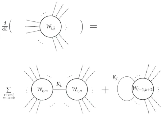
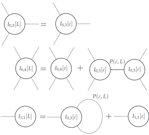
More formally,Ief f_[_L_{] can be expressed as a sum over Feynman graphs,}

where the edges are labelled by the propagator P( , L) =

! L

e− m2K and where the vertices are labelled byIef f[ ].

This effective interaction Ief f_[_L_{] is an} _!_{-dependent functional on the}

space C∞(M) of fields. We can expand Ief f_[_L_{] as a formal power series}

Ief f[L] = ' i,k≥0 !i_Ief f i,k [L] where I_i,kef f[L] :C∞(M)_→R

is homogeneous of orderk. Thus, we can think ofIi,k[L] as being a symmetric

linear map

(16)

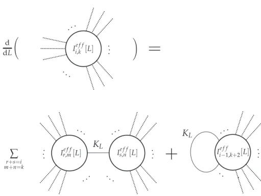
Figure 1. The first few expressions in the renormalization group flow from scale to scaleL. The dotted lines indicate incoming particles. The blobs indicate interactions between these particles. The symbol I_i,kef f[L] indicates the !i term in the contribution to the interaction of k particles at length-scaleL. The solid lines indicate the propagation of a particle between two interactions; particles are allowed to propagate with proper time between andL.

We should think of I_i,kef f[L] as being a contribution to the interaction of k particles which come together in a region of size around L.

Figure 1 shows how to express, graphically, the world-line version of the renormalization group flow.

3.6. So far in this section, we have sketched the definition of two versions of the renormalization group flow: one based on energy, and one based on length. There is a more general definition of the renormalization group flow which includes these two as special cases. This more general version is based on the concept of parametrix.

(17)

Definition 3.6.1. A parametrix for the Laplacian D on a manifold is

a symmetric distribution P on M2 _{such that} _(D_⊗₁₎_P ₋

M is a smooth function on M2 (where M refers to the -distribution on the diagonal of

M.

This condition implies that the operator ΦP :C∞(M)→C∞(M)

asso-ciated to the kernelP is an inverse for D, up to smoothing operators: both P◦D−Id and D◦P−Id are smoothing operators.

IfKtis the heat kernel for the Laplacian D, thenPlength(0, L) = &L

0 Ktdt

is a parametrix. This family of parametrices arises when one considers the world-line picture of quantum field theory.

Similarly, we can define an energy-scale parametrix Penergy[Λ,∞) =

' ≥Λ

1 e _⊗e

where the sum is over an orthonormal basis of eigenfunctions e for the Laplacian D, with eigenvalue .

Thus, we see that in either the world-line picture or the momentum scale picture one has a family of parametrices ( Plength(0, L) and Penergy[Λ,∞),

respectively) which converge (in theL_→0 and Λ_{→ ∞}limits, respectively) to the zero distribution. The renormalization group equation in either case is written in terms of the one-parameter family of parametrices.

This suggests a more general version of the renormalization group flow, where an arbitrary parametrix P is viewed as defining a “scale” of the the-ory. In this picture, one should have an effective action Ief f_[_P_{] for each}

parametrix. IfP, P!are two different parametrices, thenIef f[P] andIef f[P!] must be related by a certain renormalization group equation, which expresses Ief f[P] in terms of a sum over graphs whose vertices are labelled byIef f[P!] and whose edges are labelled byP ₋P!.

If we restrict such a family of effective interactions to parametrices of the form Plength(0, L) one finds a solution to the world-line version of the

renormalization group equation. If we only consider parametrices of the form Penergy[Λ,∞), and then define

Sef f[Λ]( ) =₋1₂

! M

D +Ief f[Penergy[Λ,∞)]( ),

for ∈C∞(M)_[0,Λ), one finds a solution to the energy scale version of the renormalization group flow.

A general definition of a quantum field theory along these lines is ex-plained in detail in Chapter 2, Section 8. This definition is equivalent to one based only on the world-line version of the renormalization group flow, which is the definition used for most of the book.

(18)

5. LOCALITY 13

4. A Wilsonian definition of a quantum field theory

Any detector one could imagine has some finite resolution, and so only probes some low-energy effective theory, described by some Sef f_[Λ].

How-ever, one could imagine building detectors of arbitrarily high (but finite) resolution, and so one could imagine probing Sef f[Λ] for arbitrarily high (but finite) Λ.

As is usual in physics, one should only consider those objects which can in principle be observed. Thus, one should say thatall aspects of a quantum field theory are encoded in its various low-energy effective theories.

Let us make this into a (rough) definition. A more precise version of this definition is given later in this introduction; a completely precise version is given in the body of the book.

Definition 4.0.2. A (continuum) quantum field theory is:

(1) An effective action

Sef f[Λ] :C∞(M)_[0,Λ]_→_R[[_!]]

for all Λ ∈ (0,∞). More precisely, Sef f[Λ] should be a formal

power series both in the field ∈ C∞(M)_[0,Λ] and in the variable

!.

(2) Modulo !, each Sef f[Λ] must be of the form Sef f[Λ]( ) =₋1₂

! M

D + cubic and higher terms.

where Dis the positive-definite Laplacian. (If we want to consider a massive scalar field theory, we can replaceD by D +m2).

(3) IfΛ!_<_Λ_, _Sef f_[Λ!_]_{is determined from} _Sef f_[Λ] _{by the} renormaliza-tion group equarenormaliza-tion (which makes sense in the formal power series setting).

(4) The effective actionsSef f_[Λ]_{satisfy a} _{locality axiom}_{, which we will} sketch below.

Earlier I described several different versions of the renormalization group equation; one based on the world-line formulation of quantum field theory, and one defined by considering arbitrary parametrices for the Laplacian. One gets an equivalent definition of quantum field theory using either of these versions of the renormalization group flow.

5. Locality

Locality is one of the fundamental principles of quantum field theory. Roughly, locality says that any interaction between fundamental particles occurs at a point. Two particles at different points of space-time cannot spontaneously affect each other. They can only interact through the medium of other particles. The locality requirement thus excludes any “spooky ac-tion at a distance”.

(19)

Locality is easily understood in the naive functional integral picture. Here, the theory is supposed to be described by a functional measure of the form

eS( )/!d ,

where d represents the non-existent Lebesgue measure onC∞(M). In this picture, locality becomes the requirement that the action function S is a

local action functional.

Definition 5.0.3. A function

S :C∞(M)→R[[_!]]

is a local action functional, if it can be written as a sum

S( ) ='Sk( ) where Sk( ) is of the form

Sk( ) = !

M

(D1 )(D2 )· · ·(Dk )dV olM where Di are differential operators on M.

Thus, a local action functional S is of the form S( ) =

! x∈ML

( )(x)

where the LagrangianL( )(x)only depends on Taylor expansion of atx.

5.1. Of course, the naive functional integral picture doesn’t make sense. If we want to give a definition of quantum field theory based on Wilson’s ideas, we need a way to express the idea of locality in terms of the finite energy effective actionsSef f_[Λ].

As Λ→ ∞, the effective actionSef f_{[Λ] is supposed to encode more and}

more “fundamental” interactions. Thus, the first tentative definition is the following.

Definition 5.1.1 (Tentative definition of asymptotic locality). A

col-lection of low-energy effective actionsSef f[Λ] satisfying the renormalization

group equation is asymptotically local if there exists a large Λ asymptotic expansion of the form

Sef f[Λ]( ).'fi(Λ)Θi( )

where theΘi are local action functionals. (TheΛ→ ∞ limit ofSef f[Λ] does not exist, in general).

This asymptotic locality axiom turns out to be a good idea, but with a fundamental problem. If we suppose that Sef f_{[Λ] is close to being local for}

some large Λ, then for all Λ! _<_{Λ, the renormalization group equation implies}

thatSef f[Λ!] is entirely non-local. In other words, the renormalization group flow is not compatible with the idea of locality.

(20)

5. LOCALITY 15

This problem, however, is an artifact of the particular form of the renor-malization group equation we are using. The notion of “energy” is very non-local: high-energy eigenvalues of the Laplacian are spread out all over the manifold. Things work much better if we use the version of the renor-malization group flow based on length rather than energy.

The length-based version of the renormalization group flow was sketched earlier. It will be described in detail in Chapter 2, and used throughout the rest of the book.

This length scale version of the renormalization group equation is essen-tially equivalent to the version based on energy, in the following sense:

Any solution to the length-scale RGE can be translated into a solution to the energy-scale RGE and conversely3_.

Under this transformation, large length will correspond (roughly) to low energy, and vice-versa.

The great advantage of working with length scales, however, is that one can make sense of locality. Unlike the energy-scale renormalization group flow, the length-scale renormalization group flow diffuses from local to non-local. We have seen earlier that it is more convenient to describe the length-scale version of an effective field theory by an effective interaction Ief f_[_L_]

rather than by an effective action. If the length-scaleLeffective interaction Ief f_[_L_{] is close to being local, then} _Ief f_[_L_{+ ] is slightly less local, and so}

on.

As L _→ 0, we approach more “fundamental” interactions. Thus, the locality axiom should say that Ief f[L] becomes more and more local as L_→0. Thus, one can correct the tentative definition asymptotic locality to the following:

Definition 5.1.2 (Asymptotic locality). A collection of low-energy

ef-fective actionsIef f_[_L_]_{satisfying the length-scale version of the} renormaliza-tion group equarenormaliza-tion is asymptotically local if there exists a smallL

asymp-totic expansion of the form

Sef f[L]( )_.'fi(L)Θi( )

where the Θi are local action functionals. (The actual L→0 limit will not exist, in general).

Because solutions to the length scale and energy scale RGEs are in bi-jection, this definition applies to solutions to the energy scale RGE as well.

We can now update our definition of quantum field theory: Definition 5.1.3. A (continuum) quantum field theory is:

(1) An effective action

Sef f[Λ] :C∞(M)_[0,Λ]_→R[[!]]

3_{The converse requires some growth conditions on the energy-scale effective actions}

(21)

for all Λ ∈ (0,∞). More precisely, Sef f[Λ] should be a formal

power series both in the field ∈ C∞(M)_[0,Λ] and in the variable

!.

(2) Modulo _!, each Sef f[Λ] must be of the form Sef f[Λ]( ) =₋1₂

! M

where Dis the positive-definite Laplacian. (If we want to consider a massive scalar field theory, we can replaceD by D +m2).

(3) IfΛ!_<_Λ_, _Sef f_[Λ!_]_{is determined from} _Sef f_[Λ] _{by the} renormaliza-tion group equarenormaliza-tion (which makes sense in the formal power series setting).

(4) The effective actions Sef f[Λ], when translated into a solution to

the length-scale version of the RGE, satisfy the asymptotic locality axiom.

Since solutions to the energy and length-scale versions of the RGE are equivalent, one can base this definition entirely on the length-scale version of the RGE. We will do this in the body of the book.

Earlier we sketched a very general form of the RGE, which uses an arbitrary parametrix to define a “scale” of the theory. In Chapter 2, Section 8, we will give a definition of a quantum field theory based on arbitrary parametrices, and we will show that this definition is equivalent to the one described above.

6. The main theorem

Now we are ready to state the first main result of this book.

Theorem A. Let T(n) denote the set of theories defined modulo !n+1. Then, T(n+1) is a principal bundle over T(n) for the abelian group of local action functionalsS :C∞(M)→R.

Recall that a functionalS is a local action functional if it is of the form S( ) =

! M

L( )

where L is a Lagrangian. The abelian group of local action functionals is

the same as that of Lagrangians up to the addition of a Lagrangian which is a total derivative.

Choosing a section of each principal bundle T(n+1) → T(n) yields an

isomorphism between the space of theories and the space of series in_!whose coefficients are local action functionals.

A variant theorem allows one to get a bijection between theories and local action functionals, once one has made an additional universal (but unnatural) choice, that of a renormalization scheme. A renormalization

(22)

6. THE MAIN THEOREM 17

scheme is a way to extract the singular part of certain functions of one variable. We construct a certain subalgebra

P((0,1))⊂C∞((0,1))

consisting of functions f( ) of a “motivic” nature. Functions in P((0,1)) arise as the periods of families of algebraic varieties over Zariski open subsets U _⊂A1_Q, such that U(R) contains (0,1). (For more details, see Chapter 2, Section 9).

Definition 6.0.4. A renormalization scheme is a subspace

P((0,1))<0 ⊂P((0,1))

of “purely singular” functions, complementary to the subspace P((0,1))_≥0 ⊂P((0,1))

of functions whose r_{→ ∞} limit exists.

The choice of a renormalization scheme gives us a way to extract the singular part of functions in P((0,1)).

The variant theorem is the following.

Theorem B. The choice of a renormalization scheme leads to a

bijec-tion between the space of theories and the space of local acbijec-tion funcbijec-tionals

S:C∞(M)→R[[_!]].

Equivalently, there is a bijection between the space of theories and the space of Lagrangians up to the addition of a Lagrangian which is a total derivative.

Theorem B implies theorem A, but theorem A is the more natural for-mulation.

There are certain caveats:

(1) Like the effective actionsSef f_{[Λ], the local action functional}_S _{is a}

formal power series both in ∈C∞(M) and in !. (2) Modulo_!, we require that S is of the form

S( ) =₋1₂

! M

There is a more general formulation of this theorem, where the space of fields is allowed to be the space of sections of a graded vector bundle. In the more general formulation, the action functionalSmust have a quadratic term which is elliptic in a certain sense.

6.1. Let me sketch how to prove theorem A. Given the action S, we construct the low-energy effective action Sef f_{[Λ] by renormalizing a certain}

functional integral. The formula for the functional integral is Sef f[Λ]( L) =!log (! H∈C∞(M)(Λ,∞) eS( L+ H)/! ) .

(23)

This expression is the renormalization group flow from infinite energy to energy Λ. This is an infinite dimensional integral, as the field H has

un-bounded energy.

This functional integral is renormalized using the technique of coun-terterms. This involves first introducing a regulating parameter r into the functional integral, which tames the singularities arising in the Feynman graph expansion. One choice would be to take the regularized functional integral to be an integral only over the finite dimensional space of fields

∈C∞(M)_(Λ,r].

Sending r → ∞ recovers the original integral. This limit won’t exist,

but one renormalizes this limit by introducingcounterterms. Counterterms are functionals SCT₍_r, _{) of both} _r _{and the field , such that the limit}

lim r→∞ ! H∈C∞(M)(Λ,r] exp #₁ !S( L+ H)− 1 !SCT(r, L+ H) $

exists. These counterterms are local, and are uniquely defined once one chooses a renormalization scheme.

The effective action Sef f[Λ] is then defined by this limit: Sef f[Λ]( L) = lim r→∞ ! H∈C∞(M)(Λ,r] exp #₁ !S( L+ H)− 1 !SCT(r, L+ H) $

6.2. In practise, we don’t use the energy-scale regulator r but rather a length-scale regulator . The reason is the same as before: it is easier to construct local theories using the length-scale regulator than the energy-scale regulator. In what follows, I will ignore this rather technical point; to make the following discussion completely accurate, the reader should replace the energy-scale regulator r by the length-scale regulator we will use later.

The countertermsSCT are constructed by a simple inductive procedure, and are local action functionals of the field ∈C∞(M).

Once we have chosen such a renormalization scheme, we find a set of counterterms SCT₍_r, _{) for any local action functional} _S_{. These}

countert-erms are uniquely determined by the requirements that firstly, the r → ∞

limit above exists, and secondly, they are purely singular as a function of the regulating parameter r.

6.3. What we see from this is that the bijection between theories and local action functionals is not canonical, but depends on the choice of a renormalization scheme. Thus, theorem A is the most natural formulation: there is no natural bijection between theories and local action functionals. Theorem A implies that the space of theories is an infinite dimensional manifold, modelled on the topological vector space of R[[!]]-valued local action functionals onC∞(M).

(24)

7. RENORMALIZABILITY 19

7. Renormalizability

We have seen that the space of theories is an infinite dimensional man-ifold, modelled on the space of _R[[_!]]-valued local action functionals on C∞(M).

A physicist would find this unsatisfactory. Because the space of theories is infinite dimensional, to specify a particular theory, it would take an infinite number of experiments. Thus, we can’t make any predictions.

We need to find a natural finite-dimensional submanifold of the space of all theories, consisting of “well-behaved” theories. These well-behaved theories will be called renormalizable.

7.1. An old-fashioned viewpoint is the following:

A local action functional (or Lagrangian) is renormalizable if it has only finitely many counterterms:

SCT(r) = '

f inite

fi(r)SCTi

In general, this definition picks out a finite dimensional subspace of the in-finite dimensional space of theories. However, it is not natural: the spe-cific counterterms will depend on the choice of renormalization scheme, and therefore this definition may depend on the choice of renormalization scheme.

More fundamentally, any definitions one makes should be directly in terms of the only physical quantities one can measure, namely the low-energy effective actionsSef f_{[Λ]. Thus, we would like a definition of}

renormalizabil-ity using only theSef f[Λ].

The following is the basic idea of the definition we suggest, following Wilson and others.

Definition 7.1.1 (Rough definition). A theory, defined by effective

ac-tionsSef f[Λ], is renormalizable if theSef f[Λ]don’t grow too fast asΛ_{→ ∞}.

However, we must measureSef f[Λ] in units appropriate to energy scale Λ. For instance, if Sef f[1] is measured in joules, then Sef f[103] should be measured in kilo-joules, and so on.

However, this change of units only makes sense on _Rn_{. Since we can}

identify energy with length−2_{, changing the units of energy amounts to}

rescaling Rn_{. In addition, the field} _∈ _C∞₍_Rn_{) can have its own energy}

(which should be thought of as giving the target of the map : _Rn _→ _R

some weight). Once we incorporate both of these factors, the procedure of changing units (in a scalar field theory) is implemented by the map

Rl:C∞(Rn)→C∞(Rn)

(25)

7.2. As our definition of renormalizability only makes sense on _Rn_{, we}

will now restrict to considering scalar field theories onRn_{. We want to}

mea-sure Sef f[Λ] as Λ→ ∞, after we have changed units. DefineRG_l(Sef f[Λ]) by

RGl(Sef f[Λ])( ) =Sef f[l−2Λ](Rl( ))

Thus, RG_l(Sef f_{[Λ]) is the effective action}_Sef f_[_l2_{Λ], but measured in units}

that have been rescaled by l.

We can use the mapRG_l to implement precisely the definition of

renor-malizability suggested above.

Definition 7.2.1. A theory{Sef f[Λ]}is renormalizable if RG_l(Sef f[Λ])

grows at most logarithmically asl_→0.

7.3. It turns out that the mapRG_ldefines a flow on the space of theories.

Lemma7.3.1. If _{Sef f[Λ]_}satisfies the renormalization group equation,

then so does {RG_l(Sef f[Λ]}.

Thus, sending

{Sef f[Λ]_{} → {}RG_l(Sef f[Λ])_}

defines a flow on the space of theories: this is thelocal renormalization group flow.

Recall that the choice of a renormalization scheme leads to a bijection between the space of theories and Lagrangians. Under this bijection, the local renormalization group flow acts on the space of Lagrangians. The con-stants appearing in a Lagrangian (the coupling concon-stants) become functions of l; the dependence of the coupling constants on the parameter l is called the function. Renormalizability means these coupling constants have at most logarithmic growth in l.

The local renormalization group flow RG_l, as l→ 0, can be interpreted

geometrically as focusing on smaller and smaller regions of space-time, while always using units appropriate to the size of the region one is considering. In energy terms, applyingRG_l asl→0 amounts to focusing on phenomena

of higher and higher energy.

The logarithmic growth condition thus says the theory doesn’t break down completely when we probe high-energy phenomena. If the effective actions displayed polynomial growth, for instance, then one would find that the perturbative description of the theory wouldn’t make sense at high en-ergy, because the terms in the perturbative expansion would increase with the energy.

7.4. The definition of renormalizability given above can be viewed as a perturbative approximation to an ideal non-perturbative definition.

Definition 7.4.1 (Ideal definition). A non-perturbative theory is

renor-malizable if, as we flow the theory under RG_l and let l_→0, we converge to

(26)

8. RENORMALIZABLE SCALAR FIELD THEORIES 21

This fixed point, if it exists, would be a scaling limit of the theory; it would necessarily be a scale-invariant theory. For instance, it is expected that Yang-Mills theory is renormalizable in this sense, and that the scaling limit is a free theory.

This ideal definition is difficult to make sense of perturbatively (when we treat_!as a formal parameter). For instance, suppose a coupling constantc changes to

c_/→l!c=c+!clogl+_{· · ·}

Non-perturbatively, we might think that !>0, so that this flow converges to a fixed point. Perturbatively, however, _! is a formal parameter, so it appears to have logarithmic growth.

Our perturbative definition can be interpreted as saying that a pertur-bative theory is renormalizable if, at first sight, it looks like it might be non-perturbatively renormalizable in this sense. For instance, if it contains coupling constants which are of polynomial growth in l, these will proba-bly persist at the non-perturbative level, implying that the theory does not converge to a fixed point.

One can make a more refined perturbative definition by requiring that the logarithmic growth which does appear is of the correct sign (thus distin-guishing between c_/→l!c andc_/→l−!c). This more refined definition leads toasymptotic freedom, which is the statement that a theory converges to a free theory as l_→0.

8. Renormalizable scalar field theories

Now that we have a definition of renormalizability, the next question to ask is: which theories are renormalizable?

It turns out to be straightforward to classify all renormalizable scalar field theories.

8.1. Suppose we have a local action functionalS of a scalar field onRn, and suppose thatS is translation invariant. We say thatS is ofdimension kif

S(Rl( )) =lkS( ).

(27)

Every translation invariant local action functional S is a finite sum of terms of dimension. For instance:

! R4 D is of dimension 0 ! R4 4 _{is of dimension 0} ! R4 3 ∂ ∂xi is of dimension −1 ! R4 2 _{is of dimension 2}

Now let us state how one classifies scalar field theories, in general. Theorem8.1.1. LetR(k)(Rn) denote the space of renormalizable scalar field theories onRn_{, invariant under translation, defined modulo} _!n+1_.

Then,

R(k+1)(Rn)→R(k)(Rn)

is a torsor for the vector space of local action functionals S( ) which are a

sum of terms of non-negative dimension.

Further, R(0)(Rn) is canonically isomorphic to the space of local action functionals of the form

S( ) =−1 2

!

Rn

D + cubic and higher terms, of non-negative dimension.

As before, the choice of a renormalization scheme leads to a section of each of the torsors R(k+1)(Rn) → R(k)(Rn), and so to a bijection between

the space of renormalizable scalar field theories and the space of series

−12 !

D +'!i_S i

where each Si is a translation invariant local action functional of

non-negative dimension, andS0 is at least cubic.

Applying this to _R4_{, we find the following.}

Corollary8.1.2. Renormalizable scalar field theories onR4, invariant

underSO(4)_{" R}4 _{and under} _{→ −} _{, are in bijection with Lagrangians of} the form

L( ) =a D +b 4+c 2

for a, b, c_∈R[[!]], where a=₋1₂modulo! and b= 0 modulo!.

More generally, there is a finite dimensional space of non-free renormal-izable theories in dimensions n= 3,4,5,6, an infinite dimensional space in dimensions n= 1,2, and none in dimensionsn >6. ( “Finite dimensional” means as a formal scheme over SpecR[[!]]: there are only finitely many

(28)

9. GAUGE THEORIES 23

Thus we find that the scalar field theories traditionally considered to be “renormalizable” are precisely the ones selected by the Wilsonian definition advocated here. However, in this approach, one has a conceptual reason for why these particular scalar field theories, and no others, are renormalizable.

9. Gauge theories

We would like to apply the Wilsonian philosophy to understand gauge theories. In Chapter 5, we will explain how to do this using a synthesis of Wilsonian ideas and the Batalin-Vilkovisky formalism.

9.1. In mathematical parlance, a gauge theory is a field theory where the space of fields is a stack. A typical example is Yang-Mills theory, where the space of fields is the space of connections on some principal G-bundle on space-time, modulo gauge equivalence.

It is important to emphasize the difference between gauge theories and field theories equipped with some symmetry group. In a gauge theory, the gauge group is not a group of symmetries of the theory. The theory does not make any sense before taking the quotient by the gauge group.

One can see this even at the classical level. In classicalU(1) Yang-Mills theory on a 4-manifold M, the space of fields (before quotienting by the gauge group) is Ω1₍_M_{). The action is}_S_{( ) =}&

Md ∗d . The highly

degen-erate nature of this action means that the classical theory is not predictive: a solution to the equations of motion is not determined by its behaviour on a space-like hypersurface. Thus, classical Yang-Mills theory is not a sensible theory before taking the quotient by the gauge group.

9.2. Let us now discuss gauge theories in effective field theory. Naively, one could imagine that to give a gauge theory would be to give an effective gauge theory at every energy level, in a way related by the renormalization group flow.

One immediate problem with this idea is that the space of low-energy gauge symmetries is not a group. The product of low-energy gauge sym-metries is no longer low-energy; and if we project this product onto its low-energy part, the resulting multiplication on the set of low-energy gauge symmetries is not associative.

For example, if g is a Lie algebra, then the Lie algebra of infinitesi-mal gauge symmetries on a manifold M is C∞(M)_⊗g. The space of low-energy infinitesimal gauge symmetries is then C∞(M)_≤Λ⊗g. In general,

the product of two functions in C∞(M)_≤Λ can have arbitrary energy; so

thatC∞(M)<Λ⊗gis not closed under the Lie bracket.

This problem is solved by a very natural union of the Batalin-Vilkovisky formalism and the effective action philosophy.

9.3. The Batalin-Vilkovisky formalism is widely regarded as being the most powerful and general way to quantize gauge theories. The first step in the BV procedure is to introduce extra fields – ghosts, corresponding

(29)

to infinitesimal gauge symmetries; anti-fields dual to fields; and anti-ghosts dual to ghosts – and then write down an extended classical action functional on this extended space of fields.

This extended space of fields has a very natural interpretation in ho-mological algebra: it describes thederived moduli space of solutions to the Euler-Lagrange equations of the theory. The derived moduli space is ob-tained by first taking a derived quotient of the space of fields by the gauge group, and then imposing the Euler-Lagrange equations of the theory in a derived way. The extended classical action functional on the extended space of fields arises from the differential on this derived moduli space.

In more pedestrian terms, the extended classical action functional en-codes the following data:

(1) the original action functional on the original space of fields; (2) the Lie bracket on the space of infinitesimal gauge symmetries, (3) the way this Lie algebra acts on the original space of fields. In order to construct a quantum theory, one asks that the extended action satisfies the quantum master equation. This is a succinct way of encoding the following conditions:

(1) The Lie bracket on the space of infinitesimal gauge symmetries satisfies the Jacobi identity.

(2) This Lie algebra acts in a way preserving the action functional on the space of fields.

(3) The Lie algebra of infinitesimal gauge symmetries preserves the “Lebesgue measure” on the original space of fields. That is, the vector field on the original space of fields associated to every infin-itesimal gauge symmetry is divergence free.

(4) The adjoint action of the Lie algebra on itself also preserves the “Lebesgue measure”. Again, this says that a vector field associated to every infinitesimal gauge symmetry is divergence free.

Unfortunately, the quantum master equation is an ill-defined expression. The 3rd and 4th conditions above are the source of the problem: the diver-gence of a vector field on the space of fields is a singular expression, involving the same kind of singularities as those appearing in one-loop Feynman dia-grams.

9.4. This form of the quantum master equation violates our philosophy: we should always express things in terms of the effective actions. The quan-tum master equation above is about the original “infinite energy” action, so we should not be surprised that it doesn’t make sense.

The solution to this problem is to combine the BV formalism with the effective action philosophy. To give an effective action in the BV formalism is to give a functionalSef f[Λ] on the energy_≤Λ part of the extended space of fields (i.e., the space of ghosts, fields, anti-fields and anti-ghosts). This

(30)

9. GAUGE THEORIES 25

energy Λ effective action must satisfy a certain energy Λ quantum master equation.

The reason that the effective action philosophy and the BV formalism work well together is the following.

Lemma. The renormalization group flow from scaleΛ to scaleΛ! carries

solutions of the energy Λ quantum master equation into solutions of the energy Λ! _{quantum master equation.}

Thus, to give a gauge theory in the effective BV formalism is to give a collection of effective actions Sef f[Λ] for each Λ, such that Sef f[Λ] satis-fies the scale Λ QME, and such that Sef f[Λ!] is obtained from Sef f[Λ] by the renormalization group flow. In addition, one requires that the effective actions Sef f[Λ] satisfy a locality axiom, as before.

This picture also solves the problem that the low energy gauge symme-tries are not a group. The energy Λ effective action Sef f_{[Λ], satisfying the}

energy Λ quantum master equation, gives the extended space of low-energy fields a certain homotopical algebraic structure, which has the following in-terpretation:

(1) The space of low-energy infinitesimal gauge symmetries has a Lie bracket.

(2) This Lie algebra acts on the space of low-energy fields.

(3) The space of low-energy fields has a functional, invariant under the bracket.

(4) The action of the Lie algebra on the space of fields, and on itself, preserves the Lebesgue measure.

However, these axioms don’t hold on the nose, but holdup to a sequence of coherent higher homotopies.

9.5. Let us now formalize our definition of a gauge theory. As we have seen, whenever we have the data of a classical gauge theory, we get an extended space of fields, that we will denote byE. This is always the space

of sections of a graded vector bundle on the manifoldM. As before, letE≤Λ

denote the space of low-energy extended fields.

Definition 9.5.1. A theory in the BV formalism consists of a set of

low-energy effective actions

Sef f[Λ] :E≤Λ→R[[!]],

which is a formal series both in E≤Λ and !, and which is such that: (1) The renormalization group equation is satisfied.

(2) Each Sef f_[Λ] _{satisfies the energy} _Λ _{quantum master equation.} (3) The same locality axiom as before holds.

(4) There is one more technical restriction : modulo_!, each Sef f_[Λ] _is of the form

(31)

where '−,−( is a certain canonical pairing on E, and Q:E → E satisfies certain ellipticity conditions.

As before, the locality axiom needs to be expressed in length-scale terms. The main theorem holds in this context also, but in a slightly modified form. If we remove the requirement that the effective actions satisfy the quantum master equation, we find a bijection between theories and local action functionals, depending on the choice of a renormalization scheme, as before. Requiring that the effective actions satisfy the QME leads to a constraint on the corresponding local action functional, which is called the

renormalized quantum master equation. This renormalized QME replaces the ill-defined QME appearing in the naive BV formalism.

Physicists often say that a theory satisfying the quantum master equa-tion is free of “gauge anomalies”. In general, an anomaly is a symmetry of the classical theory which fails to be a symmetry of the quantum theory. In my opinion, this terminology is misleading: the gauge group action on the space of fields is not a symmetry of the theory, but rather an inextricable part of the theory. The presence of gauge anomalies means that the theory does not exist in a meaningful way.

9.6. Renormalizing gauge theories. It is straightforward to gener-alize the Wilsonian definition of renormalizability (Definition 7.2.1) to apply to gauge theories in the BV formalism. As before, this definition only works on_Rn_{, because one needs to rescale space-time. This rescaling of space-time}

leads to a flow on the space of theories, which we call the local renormal-ization group flow. (This flow respects the quantum master equation). A theory is defined to be renormalizable if it exhibits at most logarithmic growth under the local renormalization group flow.

Now we are ready to state one of the main results of this book.

Theorem. Pure Yang-Mills theory on _R4_{, with coefficients in a simple} Lie algebra g, is perturbatively renormalizable.

That is, there exists a theory{S_{Y M}ef f[Λ]}, which is renormalizable, which

satisfies the quantum master equation, and which modulo ! is given by the classical Yang-Mills action.

The moduli space of such theories is isomorphic to_!R[[_!]].

Let me state more precisely what I mean by this. At the classical level (modulo_!) there are no difficulties with renormalization, and it is straight-forward to define pure Yang-Mills theory in the BV formalism4_{. Because}

the classical Yang-Mills action is conformally invariant in four dimensions, it is a fixed point of the local renormalization group flow.

One is then interested in quantizing this classical theory in a renormal-izable way.

4_{For technical reasons, we use a first-order formulation of Yang-Mills, which is}

(32)

11. OTHER APPROACHES TO PERTURBATIVE QUANTUM FIELD THEORY 27

The theorem states that one can do this, and that the set of all such renormalizable quantizations is isomorphic (non-canonically) to!R[[!]].

This theorem is proved by obstruction theory. A lengthy (but straight-forward) calculation in Lie algebra cohomology shows that the group of obstructions to finding a renormalizable quantization of Yang-Mills theory vanishes; and that the corresponding deformation group is one-dimensional. Standard obstruction theory arguments then imply that the moduli space of quantizations is_R[[_!]], as desired.

This calculation uses the following strange “coincidence” in Lie algebra cohomology: although H5(su(3)) is one-dimensional, the outer automor-phism group ofsu(3) acts on this space in a non-trivial way. A more direct construction of Yang-Mills theory, not relying on obstruction theory, is de-sirable.

10. Observables and correlation functions

The key quantities one wants to compute in a quantum field theory are the correlation functions between observables. These are the quantities that can be more-or-less directly related to experiment.

The theory of observables and correlation functions is addressed in the work in progress (CG10), written jointly with Owen Gwilliam. In this sequel, we will show how the observables of a quantum field theory (in the sense of this book) form a rich algebraic structure called afactorization algebra. The concept of factorization algebra was introduced by Beilinson and Drinfeld (BD04), as a geometric formulation of the axioms of a vertex algebra. The factorization algebra associated to a quantum field theory is a complete encoding of the theory: from this algebraic object one can reconstruct the correlation functions, the operator product expansion, and so on.

Thus, a proper treatment of correlation functions requires a great deal of preliminary work on the theory of factorization algebras and on the fac-torization algebra associated to a quantum field theory. This is beyond the scope of the present work.

11. Other approaches to perturbative quantum field theory

Let me finish by comparing briefly the approach to perturbative quantum field theory developed here with others developed in the literature.

11.1. In the last ten years, the perturbative version of algebraic quan-tum field theory has been developed by Brunetti, D¨utsch, Fredenhagen, Hollands, Wald and others: see (BF00; BF09; DF01; HW10). In this work, the authors investigate the problem of constructing a solution to the axioms of algebraic quantum field theory in perturbation theory. These authors prove results which have a very similar form to those proved in this book: term by term in !, there is an ambiguity in quantization, described by a certain class of Lagrangians.

(33)

The proof of these results relies on a version of the Epstein-Glaser (EG73) construction of counterterms. This construction of counterterms re-lies, like the approach used in this book, on working directly on real space, as opposed to on momentum space. In the Epstein-Glaser approach to renormalization, as in the approach described here, the proof that the coun-terterms are local is easy. In contrast, in momentum-space approaches to constructing counterterms – such as that developed by Bogoliubov-Parasiuk (BP57) and Hepp (Hep66) – the problem of constructing local counterterms involves complicated graph combinatorics.

11.2. Another, related, approach to perturbative quantum field the-ory on Riemannian space-times was developed by Hollands (Hol09) and Hollands-Olbermann (HO09). In this approach the field theory is encoded in a vertex algebra on the space-time manifold.

This seems to be philosophically very closely related to my joint work with Owen Gwilliam (CG10), which uses the renormalization techniques developed in this paper to produce a factorization algebra on the space-time manifold. Thus, the quantization results proved by Hollands-Olbermann should be close analogues of the results presented here.

11.3. In a lecture at the conference “Renormalization: algebraic, geo-metric and probabilistic aspects” in Lyon in 2010, Maxim Kontsevich pre-sented an approach to perturbative renormalization which he developed some years before. The output of Kontsevich’s construction is (as in (HO09) and (CG10)) a vertex algebra on the space-time manifold. The form of Kont-sevich’s theorem is very similar to the main theorem of this book: order by order in _!, the space of possible quantizations is a torsor for an Abelian group constructed from certain Lagrangians. Kontsevich’s work relies on a new construction of counterterms which, like the Epstein-Glaser construc-tion and the construcconstruc-tion developed here, relies on working in real space rather than on momentum space.

Again, it is natural to speculate that there is a close relationship between Kontsevich’s work and the construction of factorization algebras presented in (CG10).

11.4. Let me finally mention an approach to perturbative renormaliza-tion developed initially by Connes and Kreimer (CK98; CK99), and further developed by (among others) Connes-Marcolli (CM04; CM08b) and van Suijlekom (vS07). The first result of this approach is that the Bogoliubov-Parasiuk-Hepp-Zimmermann (BP57; Hep66) algorithm has a beautiful in-terpretation in terms of the Birkhoff decomposition for loops in a certain pro-algebraic group constructed combinatorially from graphs.

In this book, however, counterterms have no intrinsic importance: they are simply a technical tool used to prove the main results. Thus, it is not clear to me if there is any relationship between Connes-Kreimer Hopf algebra and the results of this book.

Renormalization and Effective Field Theory