MODERN cloud computing systems operate in a new and

A Hierarchical Approach for the Resource

Management of Very Large Cloud Platforms

Bernardetta Addis, Danilo Ardagna, Barbara Panicucci,

Mark S. Squillante,

Fellow,

IEEE, and Li Zhang

Abstract—Worldwide interest in the delivery of computing and storage capacity as a service continues to grow at a rapid pace. The complexities of such cloud computing centers require advanced resource management solutions that are capable of dynamically adapting the cloud platform while providing continuous service and performance guarantees. The goal of this paper is to devise resource allocation policies for virtualized cloud environments that satisfy performance and availability guarantees and minimize energy costs in very large cloud service centers. We present a scalable distributed hierarchical framework based on a mixed-integer nonlinear optimization of resource management acting at multiple timescales. Extensive experiments across a wide variety of configurations demonstrate the efficiency and effectiveness of our approach.

Index Terms—Performance attributes, performance of systems, quality concepts, optimization of cloud configurations, QoS-based scheduling and load balancing, virtualized system QoS-based migration policies

Ç

1

I

NTRODUCTION

M

ODERNcloud computing systems operate in a new and dynamic world, characterized by continual changes in the environment and in the system and performance requirements that must be satisfied. Continuous changes occur without warning and in an unpredictable manner, which are outside the control of the cloud provider. Therefore, advanced solutions need to be developed that manage the cloud system in a dynamically adaptive fashion, while continuously providing service and performance guarantees. In particular, recent studies [18], [9], [25] have shown that the main challenges faced by cloud providers are to 1) reduce costs, 2) improve levels of performance, and 3) enhance availability and dependability.

Within this framework, it should first be noted that, at large service centers, the number of servers are growing significantly and the complexity of the network infrastruc-ture is also increasing. This leads to an enormous spike in electricity consumption: IT analysts predict that by the end of 2012, up to 40 percent of the budgets of cloud service centers will be devoted to energy costs [13], [14]. Energy efficiency is, therefore, one of the main focal points on

which resource management should be concerned. In addition, providers need to comply with service-level agreement (SLA) contracts that determine the revenues gained and penalties incurred on the basis of the level of performance achieved. Quality of service (QoS) guarantees have to be satisfied despite workload fluctuations, which could span several orders of magnitude within the same business day [23], [14]. Moreover, if end-user data and applications are moved to the cloud, infrastructures need to be as reliable as phone systems [18]: Although 99.9 percent up-time is advertised, several hours of system outages have been recently experienced by some cloud market leaders (e.g., the Amazon EC2 2011 Easter outage and the Microsoft Azure outage on 29 February 2012, [9], [44]). Currently, infrastructure as a service (IaaS) and platform as a service (PaaS) providers include in SLA contracts only availability, while performance are neglected. In case of availability violations (with current figures, even for large providers, being around 96 percent, much lower than the values stated in their contracts [12]), customers are refunded with credits to use the cloud system for free.

The concept of virtualization, an enabling technology that allows sharing of the same physical machine by multiple end-user applications with performance guaran-tees, is fundamental to developing appropriate policies for the management of current cloud systems. From a technological perspective, the consolidation of multiple user workloads on the same physical machine helps to reduce costs, but this also translates into higher utilization of the physical resources. Hence, unforeseen load fluctua-tions or hardware failures can have a greater impact among multiple applications, making cost-efficient, dependable cloud infrastructures with QoS guarantees of paramount importance to realize broad adoption of cloud systems.

A number of self-managing solutions have been devel-oped that support dynamic allocation of resources among running applications on the basis of workload predictions.

. B. Addis is with the Dipartimento di Informatica, Universita` degli Studi di Torino, C.So Svizzera 185, Torino 10149, Italy. E-mail: addis@di.unito.it.

. D. Ardagna is with the Dipartimento di Elettronica, Informazione e Bioingegneria Politecnico di Milano, Via Golgi 42, Milano 20133, Italy. E-mail: ardagna@elet.polimi.it.

. B. Panicucci is with the Dipartimento di Elettronica e Informazione, Politecnico di Milano, and the Dipartimento di Scienze e Metodi dell’Ingegneria, Universita` di Modena e Reggio Emilia, Via Amendola 2, Reggio Emilia 42122, Italy. E-mail: barbara.panicucci@unimore.it.

. M.S. Squillante and L. Zhang are with the IBM Thomas J. Watson Research Center, Yorktown Heights, NY 10598.

E-mail: {mss, zhangli}@us.ibm.com.

Manuscript received 15 July 2012; revised 16 Nov. 2012; accepted 2 Jan. 2013; published online 9 Jan. 2013.

For information on obtaining reprints of this article, please send e-mail to: tdsc@computer.org, and reference IEEECS Log Number

TDSCSI-2012-07-0166.

Digital Object Identifier no. 10.1109/TDSC.2013.4.

Most of these approaches (e.g., [15]) have implemented centralized solutions: A central controller manages all resources comprising the infrastructure, usually acting on an hourly basis. This timescale is often adopted [8] because it represents a compromise in the tradeoff between the frequency of decisions and the overhead of these decisions. For example, self-managing frameworks [35], [8] may decide to shut down or power up a server, or to move virtual machines (VMs) from one server to another by exploiting the VM live-migration mechanism. However, these actions consume a significant amount of energy and cannot be performed too frequently.

As previously noted, cloud systems are continuously growing in terms of size and complexity: Today, cloud service centers include up to 10,000 servers [9], [25], and each server hosts several VMs. In this context, centralized solutions are subject to critical design limitations [9], [7], [53], including a lack of scalability and expensive monitor-ing communication costs, and cannot provide effective control within a 1-hour time horizon.

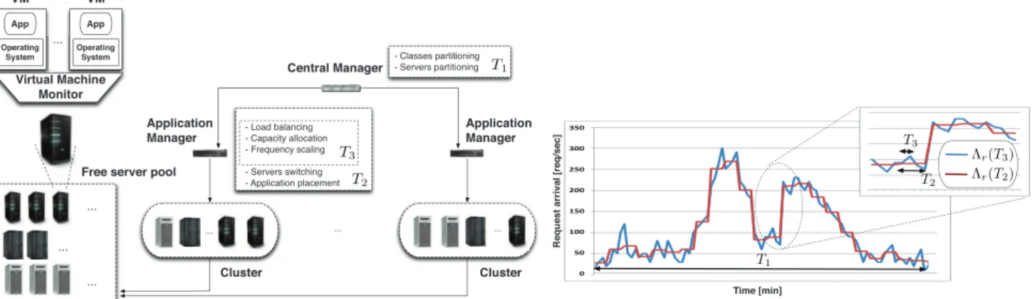
In this paper, we take the perspective of a PaaS provider that manages the transactional service applications of its customers to satisfy response time and availability guaran-tees and minimize energy costs in very large cloud service centers. We propose a distributed hierarchical framework [39] based on a mixed-integer nonlinear optimization of resource management across multiple timescales. At the root of the hierarchy, a central manager (CM) partitions the workload (applications) and resources (physical servers) over a 24-hour horizon to obtain clusters with homogeneous workload profiles one day in advance. For each cluster, an application manager (AM) determines the optimal resource allocation in a centralized manner across a subsystem of the cloud platform on a hourly basis. More precisely, AMs can decide the set of applications executed by each server of the cluster (i.e., application placement), the request volumes at various servers inside the cluster (i.e.,load balancing), and the capacity devoted to the execution of each application at each server (i.e.,capacity allocation). AMs can also decide to switch servers into a low-power sleep state depending on the cluster load (i.e.,server switching) or to reduce the operational frequency of servers (i.e., frequency scaling). Furthermore, because load balancing, capacity allocation, and frequency scaling require a small amount of time to be performed, they are executed by AMs every few (5-15) minutes. The periodicity of the placement decisions is investigated within the experimental analysis in Section 6.

Extensive experiments across a wide variety of config-urations demonstrate the effectiveness of our approach, where our solutions are very close to those achieved by a centralized method [3], [8] that requires orders of magnitude more time to solve the global resource allocation problem based on a complete view of the cloud platform. Our solution further renders net-revenue improvements of around 25-30 percent over other heuristics from the literature [41], [50], [61], [57] that are currently deployed by IaaS providers [6]. Moreover, our algorithms are suitable for parallel imple-mentations that achieve nearly linear speedup. Finally, we have also investigated the mutual influences and interrela-tionships among the multiple timescales (24 hours/1 hour/

5-15 minutes) by varying the characteristics of the prediction errors and identifying the best fine-grained timescale for runtime control.

The remainder of the paper is organized as follows: Section 2 reviews previous work from the literature, while Section 3 introduces our hierarchical framework. The optimization formulations and their solutions are presented in Sections 4 and 5, respectively. Section 6 is dedicated to experimental results, with concluding remarks in Section 7.

2

R

ELATED

W

ORK

Many solutions have been proposed for the self-manage-ment of cloud service centers, each seeking to meet application requirements while controlling the underlying infrastructure. Five main problem areas have been con-sidered in system allocation policy design:

1. application/VM placement,

2. admission control,

3. capacity allocation,

4. load balancing, and

5. energy consumption.

While each area has often been addressed separately, it is noteworthy that these problem solutions are closely related. For example, the request volume determined for a given application at a given server depends on the capacity allocated to that application on the server. A primary contribution of this paper is to integrate all five problem areas within a unifying framework, providing very efficient and robust solutions at multiple timescales.

Three main approaches have been developed: 1)control theoretic feedback loop techniques, 2)adaptive machine learning approaches, and 3) utility-based optimization techniques. A main advantage of a control theoretic feedback loop is system stability guarantees. Upon workload changes, these techniques can also accurately model transient behavior and adjust system configurations within a transitory period, which can be fixed at design time. A previous study [35] implemented a limited look-ahead controller that deter-mines servers in the active state, their operating frequency, and the allocation of VMs to physical servers. However, this implementation considers the VM placement and capacity allocation problems separately, and scalability of the proposed approach is not considered. A recent study [55], [53] proposed hierarchical control solutions, particularly providing a cluster-level control architecture that coordi-nates multiple server power controllers within a virtualized server cluster [55]. The higher layer controller determines capacity allocation and VM migration within a cluster, while the inner controllers determine the power level of individual servers. However, application and VM place-ment within each service center cluster is assumed to be given. Similarly, coordination among multiple power controllers acting at rack enclosures and at the server level is done without providing performance guarantees for the running applications [53].

Machine learning techniques are based on live system learning sessions, without a need for analytical models of applications and the underlying infrastructure. A previous study [30] applied machine learning to coordinate multiple

autonomic managers with different goals, integrating a performance manager with a power manager to satisfy performance constraints while minimizing energy expenses exploiting server frequency scaling. Recent studies provide solutions for server provisioning and VM placement [36] and propose an overall framework for autonomic cloud management [59]. An advantage of machine learning techniques is that they accurately capture system behavior without any explicit performance or traffic model and with little built-in system-specific knowledge. However, training sessions tend to extend over several hours [30], retraining is required for evolving workloads, and existing techniques are often restricted to separately applying actuation mechanisms to a limited set of managed applications.

Utility-based approaches have been introduced to optimize the degree of user satisfaction by expressing their goals in terms of user-level performance metrics. Typically, the system is modeled by means of a performance model embedded within an optimization framework. Optimiza-tion can provide global optimal soluOptimiza-tions or suboptimal solutions by means of heuristics, depending on the complexity of the optimization model. Optimization is typically applied to each one of the five problems separately. Some research studies address admission con-trol for overload protection of servers [28]. Capacity allocation is typically viewed as a separate optimization activity that operates under the assumption that servers are protected from overload. VM placement recently has been widely studied [15], [13], [20]. A previous study [61] has presented a multilayer and multiple timescale solution for the management of virtualized systems, but the tradeoff between performance and system costs is not considered. A hierarchical framework for maximizing cloud provider profits, taking into account server provisioning and VM placement problems, has been similarly proposed [14], but only very small systems have been analysed. The problem of VM placement within an IaaS provider has been considered [31], providing a novel stochastic performance model for estimating the time required for VMs startup. However, each VM is considered as a black box and performance guarantees at the application level are not provided. Finally, frameworks for the colocation of VMs into clusters based on an analysis of 24-hour application workload profiles have been proposed [26], [23], but only the server provisioning and capacity allocation problems

have been solved without considering the frequency scaling mechanism available with current technology.

In this paper, we propose a utility-based optimization approach, extending our previous works [39], [3], [8] through a scalable hierarchical implementation across multiple timescales. In particular, [39] has provided a theoretical framework investigating the conditions under which a hierarchical approach can provide the same solution of a centralized one. The hierarchical implementa-tion we propose here is built on that framework and includes the CM and the AMs, whereas in [3], [8], only a CM was considered, which implied more time to solve the global resource allocation problem as well as a complete view of the cloud platform.

To the best of our knowledge, this is the first integrated framework that also provides availability guarantees to running applications, because all foregoing work consid-ered only performance and energy management problems.

3

H

IERARCHICAL

R

ESOURCE

M

ANAGEMENT

This section provides an overview of our approach for hierarchical resource management across multiple time-scales in very large scale cloud platforms. The main components of our runtime management framework are described in Section 3.1, while our performance and power models are discussed in Section 3.2.

3.1 Runtime Framework

We assume the PaaS provider supports the execution of multiple transactional services, each representing a differ-ent customer application. The hosted services can be heterogeneous with respect to resource demands, workload intensities, and QoS requirements. Services with different quality and workload profiles are categorized into inde-pendent request classes, where the system overall serves a setRof request classes.

Fig. 1 depicts the architecture of the service center under consideration. The system includes a setSof heterogeneous servers, each running a virtual machine monitor (VMM) (such as IBM POWER Hypervisor, VMWare or Xen) configured in non-work-conserving mode (i.e., computing resources are capped and reserved for the execution of individual VMs). The physical resources (e.g., CPU, disks, communication network) of a server are partitioned among Fig. 1. Hierarchical resource management framework and interrelationship among the timescalesT1; T2, andT3.

multiple VMs, each running a dedicated application. Among the many physical resources, we focus on the CPU and RAM as representative resources for the resource allocation problem, consistent with [47], [50], [15]. Any class can be supported by multiple application tiers (e.g., front end, application logic, and data management). Each VM hosts a single application tier, where multiple VMs implementing the same application tier can be run in parallel on different hosts. Under light load conditions, servers may be shutdown or placed in a stand-by state and moved to a free server pool to reduce energy costs. These servers may be subsequently moved back to an active state and reintroduced into the running infrastructure during peaks in the load.

To go into details, we assume that each server has a single CPU supporting dynamic voltage and frequency scaling (DVFS) by choosing both its supply voltage and operating frequency from a limited set of values, noting that this single-CPU assumption is without loss of generality in heavy traffic [56] and can be easily relaxed in general. The adoption of DVFS is very promising because it does not introduce any system overhead, while hibernating and restoring a server both require time and energy. Following [43], [46], we adopt full system power models and assume that the power consumption of a server depends on its operating frequency/voltage as well as the current CPU utilization. Moreover, as in [35], [30], [24] but without limiting the generality, servers performance is assumed to be linear in its operating frequency. Finally, each physical server s has availability as, and to provide availability

guarantees, the VMs running the application tiers are replicated on multiple physical servers and work under the so-called load-sharing configuration [10].

Our resource management framework is based on a hierarchical architecture [39]. At the highest level of the hierarchy, a CM acts on a timescale of T1 (i.e., every

24 hours) and is responsible for partitioning the classes and servers into clusters one day in advance (long-term problem). The objective is to obtain a set of clustersC, each element of which has a homogeneous profile to reduce server switch-ing at finer-grained timescales. Furthermore, we denote by

Rcthe set of request classes assigned to clusterc2 Cand by St

c the set of physical servers in clustercat time intervalt.

At a lower level of the hierarchy, AMs centrally manage individual clusters acting on a timescale of T2 (i.e., on an

hourly basis). Each AM can decide (medium-term problem):

1. application placement within the cluster,

2. load balancing of requests among parallel VMs supporting the same application tier,

3. capacity allocation of competing VMs running on each server,

4. switching servers into active or low-power sleep states, and

5. increasing/decreasing the operating frequency op-eration of the CPU of a server.

Furthermore, because the load balancing, capacity alloca-tion, and frequency scaling optimization do not add significant system overhead, they are performed by AMs more frequently (short-term problem) on a timescale of T3

(i.e., every 5-15 minutes).

The decisions that take place at each timescale are obtained according to a prediction of the incoming work-loads, as in [61], [4], [16], [39], [7]. Concerning this prediction, several methods have been adopted in many fields for decades [16] (e.g., ARMA models, exponential smoothing, and polynomial interpolation), making them suitable to forecast seasonal workloads, common at time-scale T1, as well as runtime and nonstationary request

arrivals characterizing timescale T3. In general, each

prediction mechanism is characterized by several alterna-tive implementations, where the choice about filtering or not filtering input data—a runtime measure of the metric to be predicted—and choosing the best model parameters in a static or dynamic way are the most significant.

By considering multiple timescales, we are able to capture two types of information related to cloud sites [61]. The fine-grained workload traces at timescale T3 (see

also the following section) exhibit a high variability due to the short-term variations of typical web-based workloads [16]. For this reason, the finer-grained timescale provides useful information to react quickly to workload fluctua-tions. At coarser-grained timescalesT1andT2, the workload

traces are more smooth and not characterized by the instantaneous peaks typical at the finer-grained timescale. These characteristics allow us to use the medium and long timescale algorithms to predict the workload trend that represents useful information for resource management.

Note that a hierarchical approach is also beneficial to reduce the monitoring data required to compute workload predictions. Indeed, a centralized solution would require collection of central node application workloads at timescale T3. Vice versa, with a hierarchical solution AMs need to

provide aggregated data (i.e., the overall incoming work-load served for applications) of the individual managed partitions to the CM at timescaleT1.

Dependability and fault tolerance are also important issues in developing resource managers for very large infrastructures. There has been research employing peer-to-peer designs [2] or using gossip protocols [58] to increase dependability. In [2], a peer-to-peer overlay is constructed to disseminate routing information and retrieve states/ statistics. Wuhib et al. [58] propose a gossip protocol to compute, in a distributed and continuous fashion, a heuristic solution to a resource allocation problem for a dynamically changing resource demand. In our solution, to provide better dependability for the management infra-structure, each cluster maintains a primary and a backup AM. The primary and the backup do not need to be tightly synchronized to the second level, as the decisions they are making are at a timescale of 5-15 minutes. Similarly, a backup CM is also maintained in our solution. We will investigate the peer-to-peer management infrastructure as part of future work.

Finally, an SLA contract, associated with each service class, is established between the PaaS provider and its customers. This contract specifies the QoS levels that the PaaS provider must satisfy when responding to customer requests for a given service class, as well as the correspond-ing priccorrespond-ing scheme. Followcorrespond-ing [52], [11] (but without limiting the generality of our approach), for each class

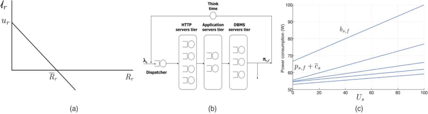
r2 R, a linear utility function specifies the per request revenue (or penalty)Ur incurred when the average

end-to-end response time Rr realizes a given value: Ur¼

rRrþur, (see Fig. 2a). The slope of the utility function is r such thatr¼ur=Rr >0, whereur is the linear utility

functiony-axis intercept andRris the threshold identifying

the revenue/penalty region, i.e., if Rr> Rr the SLA is

violated and penalties are incurred. SLA contracts also involve multiclass average response time metrics for virtualized systems (whose evaluation is discussed in the next section) and the minimum level of availability Ar

required for each service classr.

3.2 System Performance and Power Models

The cloud service center is modeled as a queuing network composed of a set of multiclass single-server queues and a delay center (see Fig. 2b). Each layer of queues represents the collection of applications supporting the execution of requests at each tier. The delay center represents the client-based delays, or think time, between the completion of one request and the arrival of the subsequent request within a session. There is a different set of application tiers Ar that

support the execution of class r requests. This section focuses on the medium-term timescale T2, noting that

similar considerations can be drawn for the timescales T1

andT3. The relationships among the timescalesT1,T2, and

T3 are illustrated in Fig. 1. We denote by nT2 (nT3) the

number of time intervals at granularity T2 (T3) within the

time periodT1 (T2), which can be expressed asnT2¼T1=T2

(nT3¼T2=T3) and assumed to be an integer.

In a given time interval, user sessions begin with a classr request arriving to the service center from an exogenous source with average rate trðT2Þ. Upon completion, the

request either returns to the system as a classr0request with probabilityr;r0or departs with probability1P_l2Rr;l. The

aggregate arrival rate for classrrequests,t

rðT2Þ, is given by

the exogenous arrival rates and transition probabilities: t

rðT2Þ ¼trðT2Þ þ

P

r0_2Rt_r0ðT2Þ r0_;r. Let _r; denote the

maximum service rate of a unit capacity server dedicated to the execution of an application of classrat tier. We assume requests on every server at different application tiers within each class are executed according to the processor sharing scheduling discipline (a common model of time sharing among web servers and application containers [4]), where the service time of classrrequests at serversfollows a general distribution having mean ðCs;fr;Þ1, withCs;f denoting

the capacity of serversat frequencyf[32], [19]. The service rates r; can be estimated at runtime by monitoring

application execution (see, e.g., [40]). They can also be estimated at a very low overhead by a combination of inference and filtering techniques developed in [60], [34], [33].

Lett

s;r; denote the execution rate for classrrequests at

tier on serversin time intervalt, and lett

s;r;denote the

fraction of VM capacity for class r requests at tier on serversin time intervalt. Once a capacity assignment has been made, VMMs guarantee that a given VM and hosted application tier will receive their assigned resources (CPU capacity and RAM allotment), regardless of the load imposed by other applications. Under the non-work-conserving mode, each multiclass single-server queue associated with a server application can be decomposed into multiple independent single-class single-server M/G/1 queues with capacity equal toCs;fts;r;. Then, the average

response time for classrrequests,Rr, is equal to the sum of

the average response times for classr requests executed at tier on server s working at frequency f, Rf

s;r;, each of

which can be evaluated as Rf_s;r;¼ 1 Cs;fr;ts;r;ts;r; Rr¼ 1 t rðT2Þ X s2S;2Ar t_s;r;Rf_s;r;: ð1Þ

Although system performance metrics have been evaluated by adopting alternative analytical models (e.g., [41], [1], [54]) and accurate performance models exist in the literature for web systems (e.g., [45], [28]), there is a fundamental tradeoff between the accuracy of the models and the time required to estimate system performance metrics. Given the strict time constraints for evaluating performance metrics in our present setting, the high complexity of analyzing even small-scale instances of existing performance models has prevented us from exploiting such results here. It is important to note, however, that highly accurate approximations for general queuing networks [22], [21], having functional forms similar to those above, can be directly incorporated into our modeling and optimization frameworks.

Energy-related costs are computed using the full system power models adopted in [43], [46], which yield server energy consumption estimate errors within 10 percent. Servers in a low-power sleep state still consume energy (cost parametercs) [35], whereas its dynamic operating cost when

running depends on a constant base costcsþps;f (function

of the operating frequency f) and an additional cost component that varies linearly with CPU utilization Us

having slopebs;f [43] (see Fig. 2c). Following [35], [50], we

further consider the switching cost css that includes

the power consumption costs incurred when starting up the server from a low-power sleep state and, possibly, the revenue lost when the computer is unavailable to perform any useful service for a period of time. Finally, to limit the number of VM movements in the system, we add a cost associated with VM movement, cm, which avoids system instability and minimizes the total number of application starts and stops [35], [50]. The costcmhas been evaluated by considering the cost of the use of a server to suspend, move and startup a VM according to the values reported in [49], [29]. Table 1 summarizes the notation adopted in this paper.

4

F

ORMULATION OF

O

PTIMIZATION

P

ROBLEMS In this section, we introduce resource management optimi-zation problems at multiple timescales (T1, T2, T3). The

general objective is to maximize profit, namely the difference between revenues from SLA contracts and costs associated with servers switching and VM migrations, while providing availability guarantees. We formulate the optimization problem at the timescale ofT2(medium-term problem) from

which, at the end of this section, will straightforwardly render the formulations at the other timescales.

As previously explained, the CM determines one day in advance the class partition Rc and the server

assignment St

c for each cluster c and every time interval

t¼1;. . .; nT2. The AM controlling cluster c has to

determine at timescale T2:

1. the servers in active state, introducing for each serversa binary variablext

sequal to 1 if serversis

running in intervaltand 0 otherwise;

2. the operating frequency of the CPU of each server, given by the binary variableyt_s;f equal to 1 if servers is working with frequency f in interval t and 0 otherwise;

3. the set of applications executed by each server, introducing the binary variablezt_s;r;equal to 1 if the application tier for classris assigned to serversin intervaltand 0 otherwise;

4. the rate of execution for classrat tieron serversin intervalt(i.e.,t

s;r;);

5. the fraction of capacity devoted to executing VM at tier for classrat serversin interval t(i.e.,t

s;r;).

We also introduce an auxiliary binary variablewt

s;requal to

1 if at least an application tier for class r is assigned to serversin intervaltand 0 otherwise.

The revenue for executing class r requests is given by T2UrtrðT2Þ ¼T2 ðurrRrÞ trðT2Þ, whereas the total

cost is given by the sum of costs for servers in the low-power sleep state, for using servers according to their operating frequency, and for penalties incurred when switching servers from the low-power sleep state to the active state while migrating VMs. Since the utilization of serverswhen it is operating at frequencyf is

TABLE 1

Us¼ X 2Ar;r2Rc t s;r; P f2FsCs;f yts;f r; ;

the profit (i.e., objective function) is given by X r2Rc r X s2St c;2Ar t s;r; P f2FsCs;fyt_s;fr;ts;r;ts;r; 0 @ 1 A 2 4 þX r2Rc urtrðT2Þ X s2St c csþ X s2St c;f2Fs ps;fyts;fþ bs;fyts;f P 2Ar;r2Rcts;r; P f2FsCs;fr;yts;f !3 5T2 X s2St c cssmax 0; xt_sxt_s1 X s2St c;r2Rc;2Ar cmmax0; zt_s;r;zt_s;r;1:

The first and second terms of the objective function are SLA revenues, the third are costs of servers in the low-power sleep state, the fourth are costs of using servers at their operating frequency, the fifth are penalties for switching servers from low-power sleep to active states, and the sixth are penalties associated with moving VMs. Note that the termsP_r2RcT2urrðT2ÞandPs2St

ccsT2can be ignored because they are independent of the decision variables. The medium-term resource allocation problemðRAPT2

c Þthat an

AM solves for its cluster c (every hour as described in Section 1) can, therefore, be formulated as follows:

maxf_ct¼ X r2Rc;s2St c;2Ar rts;r; P f2FsCs;fyt_s;f r;ts;r;ts;r; X s2St c;f2Fs ps;fyts;fþ bs;fyts;f X 2Ar;r2Rc t_s;r; P f2FsCs;fr;yts;f ! X s2St c css T2 maxð0; xt_sxt_s1Þ X s2St c;r2Rc;2Ar cm T2 maxð0; zt_s;r;zt_s;r;1Þ s:t: X s2St c t_s;r;¼t_rðT2Þ ¼t_r;ðT2Þ 8r2 Rc; 2 Ar; ð2Þ X r2Rc;2Ar t_s;r;1 8s2 Stc; ð3Þ X f2Fs yt_s;f¼xt_s 8s2 St c; ð4Þ zt_s;r; xt_s 8s2 St c; r2 Rc; 2 Ar; ð5Þ t_s;r; rðT2Þtzts;r; 8s2 S t c; r2 Rc; 2 Ar; ð6Þ t_s;r;< X f2Fs Cs;fyts;f ! r; ts;r; 8s2 S t c; r2 Rc; 2 Ar; ð7Þ X 2Ar RAMr;zts;r;RAMs 8s2 Stc; r2 Rc; ð8Þ Y 2Ar 1Y s2St c 1as ð Þwts;r 0 @ 1 AAr 8r2 Rc; ð9Þ X 2Ar zt_s;r; jArj wts;r 8s2 S t c; r2 Rc; t_s;r;; t_s;r;0; xt_s; yt_s;f; zt_s;r;; wt_s;r2 f0;1g 8s2 St c; r2 Rc; 2 Ar: ð10Þ

Constraint (2) ensures that the traffic assigned to individual servers and every application tier equals the overall load predicted for classrjobs. Note that for a given request class r, the overall load t

rðT2Þ is the same at every tier.

Constraint (3) expresses bounds for the VMs capacity allocation (i.e., at most 100 percent of the server capacity can be used). Constraint (4) guarantees that if serversis in the active state, then exactly one frequency is selected in the set Fs (i.e., only one variable yts;f is set to 1). Indeed, if

xt

s¼0, then no frequency can be selected and everyyts;f is

equal to 0, vice versa if the server is in active state and xt

s¼1, exactly one variableyts;f is set to 1. Hence, the extra

cost of a server operating at frequencyfand its correspond-ing capacity is given byP_f2Fsbs;fyts;fand

P

f2FsCs;fyts;f,

respectively. Constraint (5) states that application tiers can only be assigned to servers in the active state. Indeed, if the server is in active statext

s¼1and thenzts;r;can be raised to

one. Vice versa, if the server is in low-power sleep state xt

s¼0and all variableszts;r; are forced to 0. With the same

arguments, (6) allows executing requests only at a server to which the corresponding application tier has been assigned, (7) guarantees that resources are not saturated, (8) ensures that the memory available at a given server is sufficient to support all assigned VMs, (9) forces availability obtained by assigning servers to classr requests to be at least equal to the minimum level according to the load-sharing fault tolerance scheme [10] (we plan to consider more advanced availability models, along the lines of [37], [42], in our future work). Finally, Constraint (10) relates variableszt

s;r;

and the auxiliary variableswt

s;r. Indeed, if any application

tier of classris assigned to servers(at least one variable zt

s;r; is equal to 1), then alsowts;rhas to be equal to 1.

The medium-term problem (RAPT2

c ) is a mixed-integer

nonlinear programming problem that is particularly diffi-cult to solve when the number of variables is large, as in this case. Even if we consider the set of servers in the active state

xt¼ ðxsÞts2St

c with relative frequencies y

t_{¼ ðy}t s;fÞs2St

c;f2Fs and the assignment of applications on each server zt_¼ ðzt

s;r;Þs2St

c;r2Rc;2Arto be fixed, the problem is still difficult to solve because the objective function is not concave (see [8] for further details). To overcome this difficulty, we propose an efficient and effective heuristic approach described in Section 5.

Let us now turn to consider the short-term (RAPT3

c ) and

long-term (RAPT1_{) resource allocation problems. For every}

cluster c,ðRAPT3

c Þ results straightforwardly fromðRAPcT2Þ

upon fixing the set of servers in the active state (xt

s) and the

assignment of applications on each server (zt

s;r;,wts;r). The

decision variables are the operating frequency of servers yt

s;f, the request volumes at each server ts;r;, and the

fraction of capacity for executing each application at each servert

s;r;. The objective function and the constraints are

as in ðRAPT2

c Þ upon replacing trðT2Þ by the workload at

timescaleT3,trðT3Þ, in Constraints (2) and (6). For the

long-term ðRAPT1_{Þ problem, the CM determines the optimal}

class partition Rc and cluster-servers assignment Stc for

each time interval t¼1;. . .; nT2. In this case, all clusters c

and all time intervalst contribute to the objective function PnT2

t¼1

P

c2Cfct, where fct is the objective function of the

medium-termðRAPT2

c Þ problem.

It is worth noting that, as established in [39], because the CM objective function (i.e., the aggregation function for the entire system) is obtained as the sum of the objective functions for the individual AMs, the decentralized optimal solution obtained by our hierarchical distributed algorithm is equally as good as the optimal solution obtained by a corresponding centralized optimization approach.

5

S

OLUTION OF

O

PTIMIZATION

P

ROBLEMS

In this section, we describe an efficient and effective approach for solving the computationally hard optimization problems of the previous section. We first consider the medium-term (RAPT2

c ) and short-term (RAPcT3) resource

allocation problems, then turn to the long-term (RAPT1₎

optimization problem, and end by briefly discussing the interactions among them.

5.1 Medium- and Short-Term Solutions

In this section, we discuss the optimization techniques used for solving the medium-term (RAPT2

c ) and short-term

(RAPT3

c ) resource allocation problems. Computational

results demonstrate that only small instances of these problems can be solved to optimality with commercial nonlinear optimization packages. To handle representative cloud service center problem sizes, we develop a heuristic approach (see Algorithm 1).

Three basic components comprise our overall solution approach:

. Step 1. An initial solution for the medium-term problem is found by applying a greedy algorithm (Initial_ Solution() in Algorithm 1) whose output is the set of active servers x, their corresponding operating frequencies y, the assignment of tiers to servers z, an initial capacity allocation , and an initial load balancing vector . The details are provided in Section 5.1.1.

. Step 2. A fixed-point iteration (FPI) is used to search for improvements on the initial capacity allocation and load balancing decisions. As described in Section 5.1.2, the FPI solves the load balancing and capacity allocation problems while changing and keepingfixed, and vice versa.

. Step 3. A local search procedure iteratively improves the latest solution by exploring its neighborhood and using so-called moves. The details are discussed in Section 5.1.3.

Algorithm 1.ResourceAllocation() optimization procedure

5.1.1 Initial Solution

The process for building an initial solution (Algorithm 1, Step 1) is based on the greedy procedure greedyCore(), illustrated in Fig. 3, whose rationale is to assign application tiers to servers so that the CPU utilization of servers is lower than a given thresholdU. The value ofUis considered to be between 50 and 60 percent according to literature proposals (e.g., [17], [47]). Let Cs and bs, respectively, denote the

values of Cs;f and bs;fþps;f, for ys;f ¼1. Initially, greedy-Core()orders the application tiers according to nondecreas-ing values Wr; ¼resr;

P

2Ar1r;, where

res

r; is the

remaining workload to be allocated, and also orders the servers according to nondecreasing values of the ratio Cs=bs. Then, the procedure iteratively selects an (partially

allocated) application tier and assigns a classr request at tier to server s. The process is repeated until res_r; is completely allocated while guaranteeing that all server utilization are at mostU and that the RAM Constraint (8) and availability Constraint (9) are satisfied. A server is set to operate at the maximum frequency upon turning into the active state (Fig. 3, Steps 8-11). If possible, the workloadres_r; is allocated completely on servers, and after updating the server utilization, the next tier is selected (Fig. 3, Step 16). However, if resr; cannot be allocated completely on the

single servers, then the workload is partially assigned to the server guaranteeing the maximum utilizationU, and the remaining load (computed in Step 15) is allocated on subsequent servers. The construction of the initial solution starts at t¼1 by applying greedyCore()with all servers in clustercset to the low-power sleep state and all remaining workloads to be allocated set to the workload prediction for the time interval. Then, fort¼2;. . .; nT2, the initial solution

is constructed starting from the solution of the medium problem for time interval t1, used as input to greedy-Core(), apart from the load balancing, which is computed

proportionally to the previous solution. When this saturates a VM, the algorithm first tries to set the physical server to the maximum frequency and then, if this is not sufficient, it removes from the server a res

r; workload such that the

maximum utilization of the corresponding VM isU. The computational complexity of the greedyCore()

procedure is O max ( jScj X r2Rc jArj; X r2Rc jArj log X r2Rc jArj ! ; jScj logðjScj )! ;

where the first term is the number of assignments performed in a worst-case scenario, i.e., at each iteration the first server with sufficient RAM and residual comput-ing capacity is last in the servers ordercomput-ing. The computa-tional complexity for sorting the ordered lists of application tiers and servers is OðP_r2Rc jArj logðPr2RcjArjÞÞ and OðjScj logðjScjÞÞ, respectively.

5.1.2 The Fixed Point Iteration

Once the application tiers and operating frequencies are assigned to servers (i.e.,x,y, andzare fixed), the capacity allocation at each server and the load balancing can be improved through an FPI technique (Algorithm 1, Step 2). The idea is to iteratively identify the optimal value of one variable (or), while fixing the value of the other variable ( or ). Both problems, capacity allocation and load balancing, are separable into subproblems that can be solved independently. The solution of all these subproblems can be obtained in closed form via the Karush-Kuhn-Tucker conditions (see [8] for the details). It is also shown in [8] that 1) even if the FPI procedure is not guaranteed to converge to a global optimum, the FPI is asymptotically convergent, and

2) the number of iterations required for the FPI to converge within a precision of105 is typically between 6 and 20.

5.1.3 Neighborhood Exploration

The FPI yields a feasible solution for the problem of interest (medium or short term) that represents a local optimum with respect to the decision variables and . Since both medium-term and short-term problems are not convex, we can improve by applying a local search procedure that identifies a local optimum with respect to the integer variables x, y, and z; we then update the continuous variablesandin a greedy manner. Given a solution, the local search procedure explores its neighbor-hood NðÞ to find a better solution 0 and then iterates using Nð0Þ as the new neighborhood until no further improvement can be found.

The local search neighborhoodNðÞis defined as the set of solutions that can be obtained from solutionvia a set of moves. Clearly, the choice of moves is crucial to achieving good results with a local search procedure. The moves we consider are based on those proposed in [8], which are properly modified to take into account the availability constraints. We first describe the original moves and the modification necessary to tackle the availability constraints. We then explain how the neighborhood search can be modified to improve the exploration properties of our local search strategy. The moves are: setting a server into the active or low-power sleep state, scaling the server frequency, and reallocating tiers to servers.

Move M1: Set servers in low-power sleep state. Let Sactive

denote the set of servers in the active state. A server s2

Sactive with utilization Us2 ½minsUs; minsUs

(experimen-tally setting 2 ½1:1;1:2), is considered to belightly loaded

and a candidate for switching into the low-power sleep state. The load of such a candidate server, say^s, is allocated over the remaining servers proportional to their spare Fig. 3. Greedycore(): Application to server allocation.

capacity, where the spare capacity for tier of class r requests at server s is SCs;r;¼Csr;s;r;s;r;. Let

SCr; ¼Ps2Sactivef^sgSCs;r; be the overall spare capacity

available at the remaining servers in the active state for tier of classr. The load at server^sis (suboptimally) assigned to the remaining servers by settings;r; s;r;þs;r;^

SCs;r;

SCr; , which is then improved by solving an instance of the load balancing problem over only the subset of involved servers. The computational complexity of neighborhood exploration is OðjScj Pr2RcjArjÞ in the worst case scenario, where all

servers are in the active state and have the same utilization and every application tier is allocated on every server. Switching into the low-power sleep state and moving the load to the remaining servers reduces availability. If this reduction causes a violation of the availability constraint, then the server is not switched into the low-power sleep state, even if it is lightly loaded.

Move M2: Set servers in active state. A server s2Sactive

withUs2 ½ maxUs;maxUs, 2 ½0:9;0:95, is considered to

be abottleneckserver. To reduce load at a bottleneck server, say s1, a server in the low-power sleep state, say s2, with

RAMs2 greater or equal to the memory allocated on server

s1, is set into the active state. Server s2 applies the same

capacity allocation adopted bys1and runs at the maximum

frequency. Optimal load balancing is identified by solving an instance of the load balancing problem, considering only servers s1 and s2. The computational complexity of

neighborhood exploration is OðjScj2 Pr2RcjArjÞ, when the

system is running with jScj=2 servers in the active state

with almost the same utilization.

Move M3: Frequency scaling.This move updates the server frequency by one step, wherebottleneckserver frequency is increased and lightly loaded server frequency is decreased (only if Constraint (7) is not violated). The rationale is that the increase in cost for using resources can be balanced by improving system performance, while the energy savings can be counterbalanced by worsening response times. Since this move does not reallocate VMs, availability constraints are not violated and no modification is needed.

Move M4: Reallocation of application tiers to servers. This move seeks to reallocate application tiers to servers in the active state to find more profitable solutions. Since the FPI cannot allocate new application tiers on servers (see [8]), the goal is to look for application tiers that can be allocated on a different set of servers. If an application tier is deallocated from servers, the correspondingzvariable is set to zero and a tier that was not allowed to be executed on serversdue to a memory constraint can now be allocated to server s, exploiting these new degrees of freedom to allocate new application tiers on such servers.

To this end, we identify a destination servers1among all

the active servers swith sufficient memory capacity, such that Us< U (U2 ½50%60%). We then identify a

candi-date tierðr1; 1Þto be moved and the search continues until

an improvement is identified, where we look for a source servers2withUs2> U. Since the sum ofvariables on each

server equals 1 in the optimal solution of the capacity allocation problem (see [8]), the spare capacity required to allocateðr1; 1Þ is created by setting

s1;r;

s1;r;

Cs1r;U

for all application tiers currently executed on server s1

(i.e., guaranteeingUs1¼U). The capacity available at server

s1 for the new application tier isCs1r1;1s1;r1;1, and the

load of application tierðr1; 1Þis balanced between s1 and

s2 by solving the corresponding restricted instance of the

load balancing subproblem. The computational complexity of neighborhood exploration isOðjScj2ðPr2RcjArjÞ2Þin the

worst case scenario, where jScj servers are in the active

state, jScj=2 servers have a utilization less than U, and

memory requirements allow every application tier to be allocated on every server. If a tier is moved to a server with a lower availability or the number of physical servers supporting request classris increased, this move may lead to an availability constraint violation. In this case, the move is discarded.

5.1.4 Local Search Implementation

We are now ready to describe the overall local search procedure. Given the current solution, the Local_Search_-with-Availability()procedure (Algorithm 1, Step 7) explores its neighborhood to find the best solution in NðÞ, constructed using all moves for the medium-term problem (changed as already discussed, for availability feasibility) and only the frequency scaling moves for the short-term problem. If no further improvements can be found, the local search procedure Local_Search_withAvailability() stops at a local optimum. We then perform an FPI step (Algorithm 1, Step 8) seeking to improve the current solution: Try to escape from the current local optimum by optimally updating and , instead of approximating their values as done in the neighborhood exploration. If the FPI succeeds to find an improved solution, the Local_Search_-withAvailability() procedure starts again; otherwise, we accept the current result (Algorithm 1, Step 9). The overall procedure, however, is not finished. Note that the avail-ability constraints can be very difficult to satisfy because they conflict with the load balancing constraints and the objective function. In fact, the availability constraints seek a more fragmented load, while the objective function seeks a reduction in the number of servers. The introduction of availability constraints jeopardizes the feasible set and reduces the likelihood of moving from one feasible solution to another, possibly preventing us from reaching a good solution. Therefore, when theLocal_Search_withAvailability()

procedure fails to find an improvement, we consider a more complex process that allows a wider exploration: Local_ Search_withoutAvailability()(Algorithm 1, Step 11).

The current solution represents the best feasible solution found thus far by Local_Search_withAvailability(), and the neighborhood NðÞ is now constructed using all moves ignoring availability constraints (hence, some moves might be infeasible). All violations are recorded in a list, which will be useful in consecutive steps. By relaxing the availability constraints and creating a larger search space, we have more chances to move toward better solutions. The

Local_Search_withoutAvailability()procedure is repeated for a fixed number of iterations (Algorithm 1, Step 10), after which we must find a feasible solution through the procedure

Remove_Violations() (Algorithm 1, Step 12) to reenter the feasible region. Remove_Violations() switches additional servers into the active state to handle requests classes whose availability constraints are violated. We then repeat Local_ Search_withAvailability()followed by the FPI procedure.

We observe that switching additional servers into the active state (to remove violations) produces a worsening of the objective function value by at most the cost of those servers. However, because switching a server into the active state improves system performance and, therefore, SLA revenues, the worsening of the objective function value will be generally less than the cost of the additional servers. As shown in Section 6, when the current solution returns to the feasible region, Algorithm 1 does not get stuck in a local optima and the current solution can be further improved by the moves inLocal_Search_withAvailability().

Our strategy combines the two main features of a classical local-search strategy: Intensification and diversi-fication. Local_Search_withAvailability() performs the inten-sification step, refining the current feasible optimal solution through exploration of its neighborhood. Local_-Search_withoutAvailability() performs the diversification step, greedily improving the solution quality by allowing solutions to become infeasible.

For the short-term problem, we simply determine the load balancing, capacity allocation, and frequency scaling results because the additional system overhead is insignif-icant. The overall optimization procedure (Algorithm 1) starts from the current solution and the FPI is applied to locally improve the load balancing and capacity allocation results. Then, the local searchLocal_Search_withAvailability()

(Algorithm 1, Step 7) is started, with moves based solely on frequency scaling, followed by an FPI step (Algorithm 1, Step 8) to possibly improve the current solution as for the medium-term problem. However, because frequency scal-ing cannot introduce violations, we eliminate the Local_-Search_withoutAvailability() and Remove_Violations()

procedures. Hence, our solution scheme for the short-term problem is much easier than that for the medium-term problem, thus supporting the decision to solve the short-term problem at a finer-grain timescale.

5.2 Long-Term Solution

Our hierarchical optimization framework is composed of a CM and a set of AMs (see Section 3.1). The AM controls a subsystem of the cloud service center, operating on a cluster that includes a subset of applications and resources (physical servers). Each AM optimally assigns the available servers within its cluster to the given subset of applications, employing the algorithm described in the previous section. The CM determines the different partitions of applications and assignments of servers to each AM, where the algorithm operates at a timescale of T1 (24 hours) and plans the

resources for nT2 time intervals. More precisely, 1) at the

beginning of each day, all request classes are partitioned (i.e.,Rcdetermined) using a heuristic procedure based on a

prediction of the workload profile for the entire day, where the class partitioning considersnT2workload forecasts (one

for each hour); and 2) computing capacity is assigned to each partition at a timescale ofT2based on the workload of

each individual time interval (i.e., determineStc).

The rationale behind this class partitioning approach is to obtain an overall workload profile as homogeneous as possible. In this way, the number of server switches and VM migrations at a timescale of T2 can be reduced by

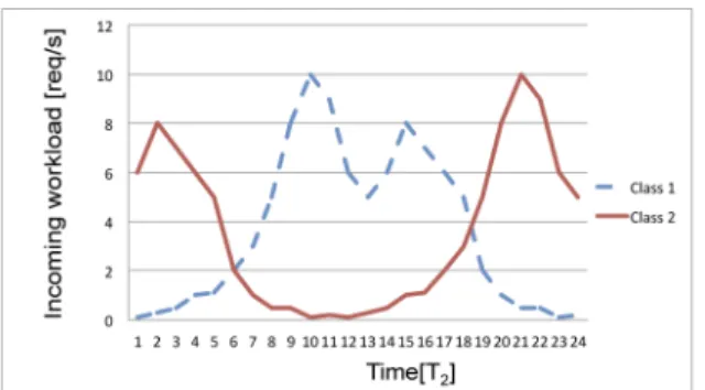
assigning to the same partition classes characterized by complementary profiles, namely classes such that when the workload of one class is at a peak, the other is at a minimum (see Fig. 4).

Another factor that needs to be carefully taken into account is the number of clusters jCj generated (or, alternatively, the maximum number of classesM included in a partition). This factor influences both the time required to find good partitions and the quality of solutions achieved by the overall framework. In fact, introducing a large number of partitions reduces the time to solve individual medium-term problems, but each cluster has a limited amount of computing capacity making the sharing of resources among classes more difficult at finer timescales. On the other hand, considering a small number of partitions, resource sharing among different classes is possible at the expense of increased execution time and complexity for the medium-term algorithm (with a limited number of clusters the framework behaves like the centralized approach characterized by large execution times that are not suitable for very large-scale service centers). The choice of a more profitable size for individual clusters has been performed experimentally and results have shown that our solution is robust with respect to this dimension (see the next section).

Our partitioning algorithm is an iterative procedure that starts from the larger set of possible partitions (i.e., where each partition contains a single class), and then iteratively tries to aggregate them two by two (see Algorithm 2). Before introducing the details of the partitioning algorithm, it is necessary to introduce some preliminary definitions. In particular, we need to introduce a similarity measure among workload profiles to implement the intuitive idea of aggregating classes with complementary profiles.

Algorithm 2. ClassPartitioning(): The class partitioning

Definition 1 (Area Under Workload Profile). Since allnT2

workload sampling steps are equal to1=T2, we define the area under the predicted workload of a request class as the area under the functiont

rðT2Þ: AðrÞ:¼ 1 T2 XnT2 t¼1 t rðT2Þ:

Definition 2 (Maximum Request Function). This function

represents, for a given set of classesPn, the maximumrðtÞat every time intervaltamong the classesr2Pnin the partition, defined as gðPn; tÞ:¼maxr t_rðT2Þ; r2Pn :

Let AðgðPnÞÞdenote the area under the above function,

omitting the time argument for simplicity.

Definition 3 (Area Summation). The area summation of

classes partition Pn, AðPnÞ, at the current iteration of the partitioning algorithm is defined as the summation of areas under the workload profile of the classes assigned toPnin the previous iterations. We, therefore, have

AðPnÞ:¼ X r2Pn AðrÞ; AðPi[PjÞ:¼ X r2Pi[Pj AðrÞ ¼AðPiÞ þAðPjÞ;

where the latter equation follows by Definition 3. Upon clustering two classes into a partition, we seek to overlay the peaks of one class with the valleys of another class so that resources unused by the first class can serve requests from the second class, and vice versa. More generally, we need to decide whether to merge two subsets of classes into a partition. To quantify the desirability of merging two sets of classes, we define the area ratio criterion as follows:

Definition 4 (Area Ratio).LetPiandPjbe two sets of request

classes. Then, the area ratio is given by

ARðPi; PjÞ:¼AðgðPi[PjÞÞ=AðPi[PjÞ:

The area ratio is based on relationships between the maximum request function and the area summation. If we evaluate whether to merge sets of classes Pi and Pj

whose workload profiles are similarly distributed, then the maximum request function is only slightly modified while the area summation is increased by AðPjÞ. Instead, if two

partitions of classes with complementary distributions are evaluated, the maximum request function of their union is (approximately) the sum of the maximum request function of the two partitions, while the area summation always increases by the same value, thus maximizing the ratio.

Let us consider the example workload profiles reported in Fig. 5. Intuitively, clustering classes 1 and 3 is less desirable than clustering classes 1 and 2 (which are complementary). It is easy to verify that the area ratio in the former case equals 0.5, while in the latter case we have an area ratio equal to 1.

We can now consider the partitioning procedure outlined in Algorithm 2. First, construct the list of actual partitions (L1) and initialize it with partitions formed by a single class

(Step 3). Then, we construct another list (L2) with all pairs of

partitions formed by elements ofL1and evaluate their area

ratio (Steps 4-5). Elements are inserted toL2in

nondecreas-ing area ratio order (Step 5), and the iterative procedure of merging partitions begins. We try to merge partitions according to two criteria: AR is above a threshold T

(T ¼0:7, chosen experimentally) and the cardinality of the new partition is less than M. Hence, we avoid creating partitions that are too large or not profitable with respect to AR. In choosing the pair of partitions following the list order, we try to merge partitions that will have the best AR. Every time a new partition is formed, it is inserted inL1and

the resulting new pairs obtained with this partition are added toL2, recalculating the AR value (Steps 11-15). The

algorithm stops when there are no more partitions that can be merged. The final partitionP determined at the end of Algorithm 2 identifies the requests class partitionfRcgused

as input by the medium-term algorithm.

The computational complexity of Algorithm 2 isOðjRj3Þ. In the worst case, therepeat-untilcycle is performedjRj=M times (recall that initially we havejRjpartitions, each one including a single class) and only one class is merged in the new partition at each iteration. The inner cycles include

jRj2pairs in the first iteration,ðjRj 1Þ2in the second, and

ðjRj jRj=Mþ1Þ2in the last.

Fig. 5. Example of workloads for the evaluation of the AR criteria. Fig. 4. Example of request classes with complementary workload profiles.

After assigning classes to partitions, the CM determines the set of servers Stc assigned to each cluster c and time

interval t, while optimizing resource allocation across successive time intervals. An initial solution is found using theInitial_Solution()procedure in Algorithm 1, and then this solution is improved through a local search phase. The local search, using servers from the Free Server Pool and/or moving servers from one partition to another, tries to add or remove capacity to partitions. The CM considers three types of moves and neighborhoods for this local search phase, where each neighborhood is explored in succession to find additional solution improvements. The neighborhoods are explored in a circular fashion (after the last neighborhood, the first one is explored again), until no further improve-ment can be found. The quality of the solutions is based on the their expected revenue, which is calculated as part of the medium-term algorithm (AM) under the workload profile forecast for the given time interval. To reduce the computational time, a simplified version of the medium-term algorithm is used where only server on/off moves are allowed. Several AMs are run in parallel, thus exploiting current multicore architectures.

The first and second types of moves increase and decrease the elaboration of resource capacity, respectively, by moving servers from theFree Server Poolto partitions or moving servers from partitions to the Free Server Pool. The third type of moves focuses on resource sharing, allowing different partitions to exchange some of the allocated capacity. The set of servers identified in this way, Stc, is

assigned at each time interval t to each cluster c for the following day.

5.3 Combined Solution

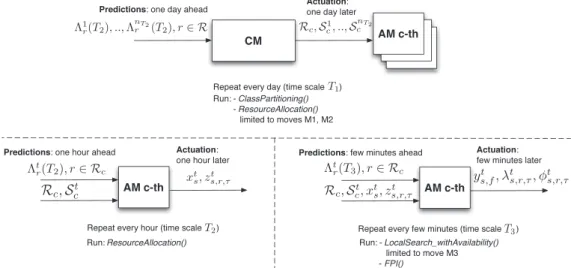
In Fig. 6, we summarize how the different components of our hierarchical solutions interact. The CM, using predic-tions of the workload one day ahead, determines the application class request partitions (Rc) and assigns them

to the different AMs. The sets of servers that will be controlled by individual AMs for each time interval (Stc

with t¼1;. . .; nT2) are also identified. The

ClassPartition-ing() procedure and the ResourceAllocation() procedure exploit only a subset of moves (Moves M1 and M2) in this

phase. The decisions will be actuated in the following day. Then, at runtime, each AM solves a series of optimization problems of type ðRAPT2

c Þ, one for each time interval in

1;. . .; nT2 using as workload estimates the predictions that

can be achieved from runtime monitoring data 1 hour in advance. At timescaleT2, the full algorithm ResourceAlloca-tion() is executed and the active servers and application placements choosen at this stage are held fixed for the following hour. Finally, at timescaleT3, each AM solves the

problem ðRAPT3

c Þ considering as decision variables only

capacity allocation, load balancing, and CPUs frequency, because they introduce a very small system overhead. Control decisions are achieved considering short-term workload predictions rðT3Þ and executing a simplified

version of the local search algorithm (i.e., LocalSearch_-withAvailability() limited to frequency scaling operations and the FPI() procedure).

Note that AMs execute the medium- and short-term algorithms, possibly with the more accurate predictions of the incoming workloadt

rðT2Þ andtrðT3Þas input relative

to the same estimates evaluated one day or one hour ahead, respectively. If an AM acting at the timescales T2 or T3

cannot find a feasible solution, then a recovery algorithm executing the fullResourceAllocation()procedure is executed with an additional set of servers. We assume that additional servers are always available in theFree Server Pooland that a feasible solution can be always found, i.e., the service center is overprovisioned.1

6

N

UMERICAL

A

NALYSIS

Our hierarchical framework has been implemented in Java and the bytecode has been optimized through the Sun Java 1.6 just in the time compiler. The resource management algorithms have been evaluated under a variety of systems and workload configurations. Section 6.1 presents the settings for our experiments, while Section 6.2 reports on the scalability results for our algorithms. Section 6.3 Fig. 6. Interactions among individual solution components at multiple timescales.

1. In the opposite case, our algorithms can provide valuable information to service centers operators on the clusters and request classes that lead to infeasibility, i.e., our solution would help to plan for investments on new servers or to identify request classes with critical SLAs.

evaluates the impact of availability constraints on the net revenues for the PaaS provider and compares the solution proposed in this paper with our previous work [8]. Section 6.4 analyzes the interrelationships among the multiple timescales considered in this paper with respect to the incoming workload prediction error. Finally, Sec-tion 6.5 presents a cost-benefit evaluaSec-tion of our soluSec-tion in comparison with other heuristics and state-of-the-art techniques [50], [41], [61], [57], [6].

6.1 Experimental Settings

Experimental analyses have been performed considering synthetic workloads built from the trace of requests registered at an IBM data center and, for the analysis in Section 6.3, at the website of a large university in Italy. The IBM data center traces dump the memory and CPU utilization of over 10,000 customer VMs running development, test, and production servers of multitiers Internet-based systems, gathered for three months during 2010 at a timescale of 15 minutes. From the CPU utilization, we derived the incoming loadrby applying the utilization

law [19], i.e., by assuming that the workload was propor-tional to the CPU usage. The university website trace contains the number of sessions registered over 100 physical servers for a 1 year period in 2006, on an hourly basis.

Data collected from the logs have been interpolated linearly and oversampled adding also some noise to obtain workload traces varying every 5, 10, and 15 minutes, as in [35]. Realistic workloads are built assuming that the request arrivals follow nonhomogeneous Poisson processes and extracting the requests traces corresponding to the days with the highest workloads experienced during the ob-servation periods.

All tests have been performed on an Intel Nehalem dual socket quad-core CPUs @2.4 GHz with 24 GB of RAM running Ubuntu Linux 2011.4 considering a large set of randomly generated instances. The performance para-meters of the applications and infrastructural resources costs have been randomly generated uniformly in the ranges reported in Table 2, as in [4], [8], [3], [35], according to commercial fees applied by IaaS/PaaS Cloud providers [5], [38] and the energy costs available in the literature [27]. The number of servers jSj has been varied between 20 and 7,200. The number of servers is scaled with the workload to obtain an average servers utilization equal to 80 percent when the workload due by the whole set of

classes reaches the peak over the 24 hours. The number of request classesjRjhas been varied between 20 and 720 and the maximum number of tiers jArj has been varied

between 2 and 4. In each test case, the number of tiers

jArjfor different classes may be different. In this way, we

can consider the execution of both the front end and back end of simple applications deployed in the cloud (e.g.,web

and Worker rolesin Microsoft Azure terminology [38]) but also more complex systems exploiting advanced middle-ware solutions available in PaaS offerings (e.g., Windows Azure Queues and Amazon SQS [5]), involving a larger number of tiers. The value range adopted forr allows us

to obtain revenues for running a service application on a single CPU for 1 hour varying between $1 and $10 according to the current commercial fees (see, e.g., the Amazon RDS service based on Oracle hosted on Amazon EC2, http://aws.amazon.com/rds/). Rr is proportional to

the number of tiersjArjand to the overall demanding time

at various tiers of classrrequests (i.e.,Rr¼10P2Ar1r;). Servers with six P-states (a voltage and frequency setting) have been considered (the working operating frequencies were 2.8, 2.4, 2.2, 2.0, 1.8, and 1.0 GHz, which implies 95-, 80-, 66-, 55-, 51-, and 34-W power consumption, according to the energy models provided in [43]). The overhead of the cooling system has been included in the data center PUE according to the values reported in [27] and the cost of energy per kWh has been varied between 0.05 and 0.25 $/kWh. The switching cost of serverscsshas

been evaluated as in [35] considering the reboot cost in energy consumed, while the cost associated with VMs movementcmhas been obtained as in [49].

The comparison of different solutions is based on the evaluation of the response times through M/G/1 models and considering the objective function values at multiple timescales. The validation of the medium- and short-term techniques in a real prototype environment has been reported in [8].

6.2 Algorithms Performance

Table 3 reports the average optimization time required by our resource management algorithms for problem instances of different sizes. The average values reported in this section have always been computed by considering 10 in-stances with the same size. Results show that the short-term algorithm is very efficient and can solve problem instances up to 120 classes and 1,200 servers in less than 1 minute.

TABLE 2

Performance Parameters and Time Unit Cost Ranges

TABLE 3

Conversely, considering the 1-hour time constraint, which characterizes the medium-term control implemented in modern cloud service centers, the medium-term algorithm can solve systems with up to 100 classes and 1,000 servers, motivating the implementation of a hierarchical approach. As for the long-term solution, problem instances including 720 classes, 7,200 servers, and around 60,000 VMs can be solved in about 16 hours; hence, the long-term algorithm is suitable for the one day ahead planning.

To estimate the speedup and the precision of our hierarchical framework with respect to the centralized approach, we have compared the solution achieved by the long-term algorithm with the solution of the medium-term algorithm without any optimization time limit. Results are reported in Table 4 and show how for small systems (up to 40 classes and 400), the hierarchical algorithm introduces a significant overhead, because the speedup (evaluated as ratio between the optimization times of the medium-term and long-term algorithms) is less or equal to 1. Increasing the size of the systems, the speedup also increases reaching a value close to 8, which is the theoretical speedup that can be achieved in the system supporting our experiments. Furthermore, the gap between the objective functions of the centralized solution computed over the 24-hour period and the long-term algorithm is about 10 percent. This gap can be motivated by the fact that in the hierarchical framework the physical servers are partitioned among the clusters, while in the centralized solution without any time limit the physical

servers can be shared among multiple classes, and hence, the centralized solution has a larger set of degrees of freedom performing the search. However, this lack of precision in the solution is significantly counterbalanced by the speedup achieved by the hierarchical framework, which is suitable for the resource management of very large-scale cloud service centers.

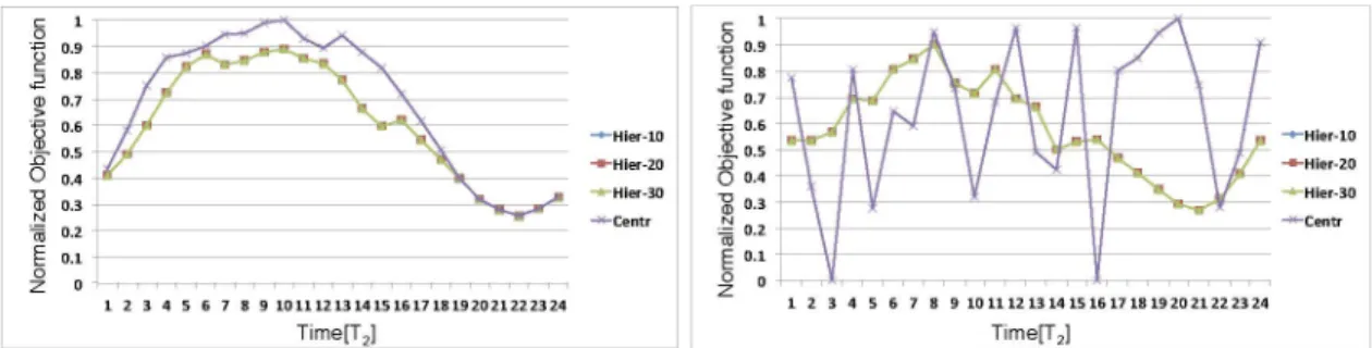
We have also investigated, the optimal number of classes Mto be included in the individual clusters managed by the AMs. In particular, we have considered clusters with 10, 20, and 30 request classes per AM. Figs. 7 and 8 report the normalized objective function value and the optimization times over the 24 hours of some representative test cases with 20, 40, and 100 classes and 200, 400, and 1,000 servers. Results show that our solution is robust to the variation of the parameter M. In the following sections, we will set M¼10, because in this way the medium-term algorithm is slightly more efficient and can compute an optimal solution in less than 1 minute (see Table 3) and can be used effectively at runtime as the recovery algorithm. Hence, if the short-term algorithm cannot find a feasible solution, the medium-term algorithm can be triggered at runtime by the AMs and a new cluster configuration can be determined by exploiting the full set of actuation mechanisms available to the system (i.e., including server switches and VM migra-tions) in case of workload fluctuations or to compensate for workload prediction errors.

As a final consideration, in Fig. 7, we report a zero optimization time for the centralized approach, if the medium-term algorithm without any time limit cannot identify a feasible solution. This plot shows that even for small-sized systems (including 40 classes and 400 servers) in heavy workload conditions, the centralized approach some-times cannot find a feasible solution. Conversely, across the entire set of experiments that we performed, the hierarchical framework always identified a feasible solution. Hence, the partitioning approach is also effective in identifying feasible solutions under critical workload conditions.

TABLE 4

Performance of the Hierarchical Algorithm

Fig. 7. Normalized objective function value for a service center with 20 classes and 200 servers (left) and 40 classes and 400 servers (right).