Dissertations (2009 -) Dissertations, Theses, and Professional Projects
Structural-Functional Brain Connectivity
Underlying Integrative Sensorimotor Function
After Stroke
Benjamin Thomas Kalinosky Marquette University
Recommended Citation
Kalinosky, Benjamin Thomas, "Structural-Functional Brain Connectivity Underlying Integrative Sensorimotor Function After Stroke" (2016).Dissertations (2009 -).Paper 616.
by
Benjamin T. Kalinosky, B.S.
A Dissertation submitted to the Faculty of the Graduate School, Marquette University,
in Partial Fulfillment of the Requirements for the Degree of Doctor of Philosophy
Milwaukee, Wisconsin
STRUCTURAL-FUNCTIONAL BRAIN CONNECTIVITY UNDERLYING INTEGRATIVE SENSORIMOTOR FUNCTION AFTER STROKE
Benjamin T. Kalinosky, B.S.
Marquette University, 2016
In this dissertation research project, we demonstrated the relationship between the structural and functional connections across the brain in stroke survivors. We used this information to predict arm function in stroke survivors, suggesting that the tools
developed through this research will be useful for prescribing individualized
rehabilitation strategies in people after stroke. Current clinical methods for rehabilitating sensorimotor function after stroke are not based on the locus of injury in the brain. Instead, therapies are generalized, treating symptoms such as weakness and spasticity. This results in outcomes that are highly variable, with severity of impairment
immediately following stroke as the best predictor of recovery. By using measures of brain structural and functional relations, we can better prognosticate and plan
rehabilitation interventions.
This research study utilized diffusion and functional magnetic resonance imaging (MRI) to quantify anatomical connectivity and functional networks of the brain after stroke. In the first aim, diffusion MRI was used to track the white matter pathways throughout the entire brain. A new imaging biomarker sensitive to stroke lesions was developed that quantifies the level of anatomical connections between every point in the brain. It was found that cortical areas most responsible for integration of sensorimotor and multisensory integration were the best predictors of motor impairments in chronic stroke subjects. Our second aim investigated the role of multisensory integration during sensorimotor control in healthy adults and stroke survivors. A novel functional MRI task paradigm involving wrist movement was developed to gain insight into the effects of multimodal sensory feedback on brain functional networks in stroke subjects. We found that the loss of functional interactions between the cerebellum and lesioned sensorimotor area were correlated with loss of movement function. Our final aim investigated the relationship between structural and functional connectivity after stroke. A model that marries diffusion MRI fiber tracking and resting-state functional MRI was designed to enhance indirect functional connections with structural information. The technique was capable of detecting changes in cortical networks that were not seen in functional or structural analysis alone. In conclusion, structure is essential to functional networks and ultimately, recovery of functional movements after stroke.
Benjamin T. Kalinosky, B.S.
Dr. Brian D. Schmit has been a great mentor. He is the embodiment of
outstanding. I would like to thank Mary Wesley for being extremely helpful. My family
has kept me alive. I thank God for them. I would also like to thank everyone in the
Integrated Neural Engineering and Rehabilitation Laboratory (INERL) for their
assistance in pilot experiments, feedback at lab meetings, and fellowship. Dr. Sheila
Schindler-Ivens and Dr. Nutta-on Promjunyakul collected the data used in my first aim.
Dr. Reivian Berrios completed the clinical assessments in my second two aims.
I am honored to have had a PhD committee of rock stars, including Dr. Scott
Beardsley, Dr. Peter LaViolette, Dr. Tugan Muftuler, Dr. Christopher Pawela, Dr. Sheila
Schindler-Ivens, and Dr. Taly Gilat-Schmidt. They provided me with excellent feedback
ABSTRACT ... i
ACKNOWLEDGEMENTS ... i
TABLE OF CONTENTS ... ii
LIST OF FIGURES ... viii
LIST OF TABLES ... vii
CHAPTER 1 : INTRODUCTION & BACKGROUND ... 1
1.1 THESIS STATEMENT ... 1
1.2 IMPAIRMENT AND RECOVERY OF MOTOR FUNCTION AFTER STROKE ... 1
1.2.1 Neurophysiology of an infarct ... 1
1.2.2 Neural basis of sensorimotor impairments after stroke ... 2
1.2.3 Neural plasticity following stroke ... 3
1.3 NEURAL MECHANISMS IN SENSORY INTEGRATION AND MOVEMENT ... 4
1.3.1 Sensorimotor and multisensory integration ... 4
1.4 MAGNETIC RESONANCE IMAGING ... 7
1.4.1 The MRI Signal... 7
1.5 DIFFUSION MRI OF WHITE MATTER ... 8
1.5.1 Diffusion-weighted MRI ... 8
1.5.2 Diffusion anisotropy in white matter ... 9
1.5.3 Models for fiber orientation ... 10
1.5.4 Tractography ... 11
1.6 STRUCTURAL CONNECTIVITY... 13
1.7 FUNCTIONAL MRI OF GRAY MATTER ... 13
1.7.3 Slice-time correction, motion correction, detrending ... 14
1.8 FUNCTIONAL CONNECTIVITY ... 16
1.8.1 Correlation-based Functional Connectivity ... 16
1.8.2 Independent Component Analysis ... 16
1.9 STRUCTURAL AND FUNCTIONAL BRAIN NETWORKS ... 17
1.9.1 Human Connectome... 17
1.9.2 Predicting function from structure ... 18
1.9.3 Structure-function relationship in plasticity after stroke ... 18
1.10 IMAGING BIOMARKERS IN STROKE ... 19
1.10.1 Diffusion MRI ... 19
1.10.2 Functional MRI ... 19
1.10.3 Personalized rehabilitation based on network models ... 20
1.11 SPECIFIC AIMS ... 20
1.11.1 AIM 1: Determine whether full brain white matter structural connectivity can predict motor impairment in chronic stroke. ... 21
1.11.2 AIM 2: Show that functional connectivity underlying sensorimotor and multisensory integration is associated with motor function after stroke. ... 21
1.11.3 AIM 3: Demonstrate the relationship between resting-state cortical networks and their anatomical connections in chronic stroke survivors. ... 22
CHAPTER 2 : WHITE MATTER STRUCTURAL CONNECTIVITY IS ASSOCIATED WITH SENSORIMOTOR FUNCTION IN STROKE SURVIVORS ... 23
2.1 INTRODUCTION ... 23
2.2 METHODS ... 26
2.3 RESULTS ... 44
2.3.1 Comparison of VISC, fiber count, and mean fiber length ... 44
2.3.2 Weak correlations of FA with VISC, mean fiber length, and fiber count ... 44
2.3.3 Tractography minimum FA stopping criterion correlates with VISC ... 45
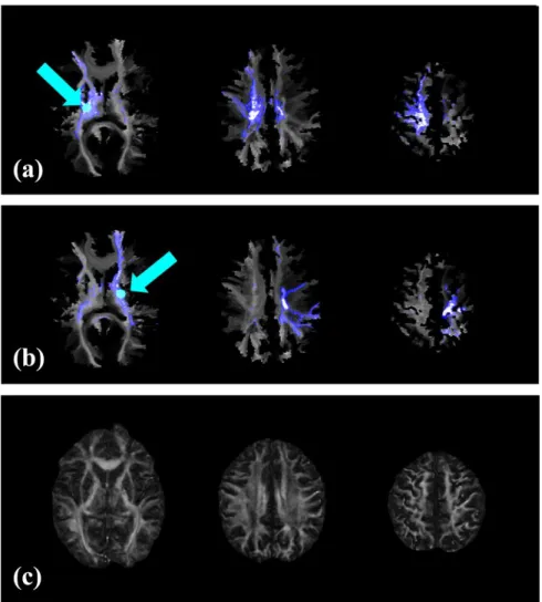
2.3.4 VISC highlighted brain areas distant from the lesion ... 47
2.3.5 VISC metric enhances lesion-related differences ... 51
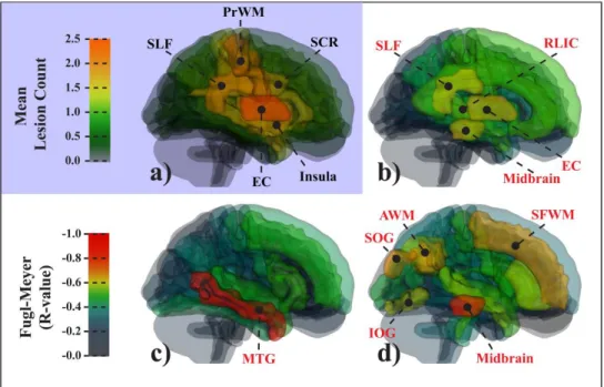
2.3.6 Whole-brain VISC correlates with Fugl-Meyer score ... 52
2.3.7 Association between VISC and Fugl-Meyer Score ... 54
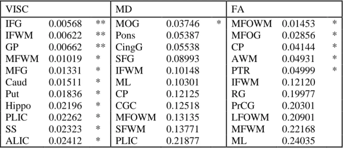
2.3.8 Post-hoc region-based results ... 56
2.4 DISCUSSION AND CONCLUSIONS ... 58
2.5 ACKNOWLEDGEMENTS ... 67
2.6 APPENDIX – Voxel-wise Indirect Structural Connectivity Derivation ... 67
CHAPTER 3 : CEREBELLAR FUNCTIONAL CONNECTIVITY IN MULTISENSORY INTEGRATION DURING MOVEMENT AFTER STROKE ... 71
3.1 INTRODUCTION ... 71
3.2 METHODS ... 75
3.2.1 Data Collection ... 75
3.2.2 Image registration and lesion side normalization ... 81
3.2.3 fMRI data processing ... 82
3.2.4 Statistical analyses ... 88
3.3 RESULTS ... 90
3.3.1 The search task produced cortical activation patterns within motor control and multisensory integration areas. ... 90
survivors depends on sensory feedback modality. ... 91
3.3.3 Stroke subjects have increased contralesional involvement within the task-related sensorimotor network ... 93
3.3.4 Stroke survivors have decreased interhemispheric connectivity and increased intrahemispheric functional connectivity to visual areas. ... 96
3.3.5 Decreased functional connectivity with the cerebellum during sensorimotor integration correlates with motor impairment after stroke. ... 97
3.4 DISCUSSION AND CONCLUSIONS ... 101
CHAPTER 4 : STRUCTURO-FUNCTIONAL CONNECTIVITY REVEALS GREATER IMPACT OF STROKE LESIONS ... 105
4.1 INTRODUCTION ... 105
4.2 METHODS ... 108
4.2.1 Data Collection ... 108
4.2.2 MRI Data Processing ... 110
4.2.3 Statistical Analysis ... 118
4.3 RESULTS ... 120
4.3.1 Stroke survivors have decreased global structural-functional connectivity. ... 120
4.3.2 Additional stroke-related differences in functional connectivity can be delineated with information provided by SFC at different fiber-lengths. ... 123
4.3.3 Structural-functional correlation enhanced areas of the brain within each resting-state network. ... 124
4.3.4 The prefrontal cortex decreases its functional connectivity with its long-distance structural connections after stroke. ... 127
4.3.5 The cerebellum has decreased functional connectivity with structural connections to the prefrontal cortex. ... 127
5.1 SUMMARY OF RESULTS ... 135
5.1.1 Brief Summary ... 135
5.1.2 Potential new insights into brain plasticity and motor recovery ... 136
5.1.3 Translation to personalized rehabilitation strategies... 137
5.2 FUTURE INVESTIGATIONS ... 138
CHAPTER 6 : APPENDIX ... 139
6.1 VISC intersession and intersubject reproducibility ... 139
6.2 Head motion and task performance differences in stroke subjects .. 142
Table 2-1: Description of the Fugl-Meyer scoring system used in this study. ... 29
Table 2-2: Descriptive characteristics of stroke survivors. ... 30
Table 2-3: Subject information. ... 51
Table 2-4: Clinical Correlations with Region-based Mean. ... 56
Table 2-5: Clinical Correlations with Region-based Difference Volume. ... 57
Table 3-1: Locations used for seed-based FC analysis. ... 88
Table 3-2: Localized group differences in BOLD activation. ... 93
Table 3-3: Localized group differences in network spatial maps. ... 96
Table 4-1: Stroke subject information ... 109
Table 4-2: Localized changes the structuro-functional correlation maps. ... 123
Figure 2-1: Overview diagram of image processing... 32
Figure 2-2: Stroke image registration. ... 35
Figure 2-3: Example calculation for VISC. ... 38
Figure 2-4: VISC correlations and contrasts. ... 46
Figure 2-5: Changes in VISC distant from a lesion ... 47
Figure 2-6: Region-based difference volume versus Fugl-Meyer score ... 49
Figure 2-7: Region-based metric means versus Fugl-Meyer score. ... 50
Figure 2-8: Scatterplot of log difference volume versus Fugl-Meyer. ... 52
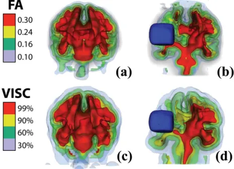
Figure 2-9: 3D isosurfaces of VISC and FA ... 53
Figure 2-10: Scatter plots of mean FA and VISC versus Fugl-Meyer score. ... 55
Figure 2-11: Scatter plots of VISC differences versus clinical score. ... 55
Figure 3-1: Task paradigm for wrist movement and sensorimotor integration. ... 77
Figure 3-2: Search-task BOLD activation maps in healthy individuals. ... 91
Figure 3-3: BOLD activation maps of stroke versus controls. ... 92
Figure 3-4: Stroke versus controls functional network maps. ... 95
Figure 3-5: Group differences in functional connectivity. ... 98
Figure 3-6: Functional trends in seed-based functional connectivity. ... 99
Figure 3-7: Scatterplots of seed-based connectivity versus motor function. ... 100
Figure 4-1: Example of SFC calculation. ... 115
Figure 4-2: Intrinsic structuro-functional correlation in stroke and controls. ... 121
Figure 4-3: Scatter plots of clinical correlations with iSFCmax. ... 122
Figure 4-6: 3D visualization of functional trends in SFC-enhanced networks. ... 128
Figure 5-1: SFC motor network in lowest functioning stroke subject. ... 137
Figure 5-2: Personalized rehabilitation with SFC networks. ... 138
Figure 6-1: Intersession reproducibility of FA and VISC for one subject. ... 141
Figure 6-2: Coefficient of variation of FA and VISC in stroke and controls. ... 141
CHAPTER 1: INTRODUCTION & BACKGROUND
1.1 THESIS STATEMENT
Changes in integrative structural and functional brain networks after stroke can
predict functional outcomes.
1.2 IMPAIRMENT AND RECOVERY OF MOTOR FUNCTION AFTER STROKE
1.2.1 Neurophysiology of an infarct
Stroke is an event of massive cell death within the brain that results from
hemorrhage or a blockage of blood from reaching the neurons. Ischemic stroke is
commonly caused by an embolism of the internal carotid artery. Atherosclerotic plaques
collect in the blood vessels, producing conditions that precede a stroke.
In the acute phase after stroke, there is an area around the lesion with reduced
water diffusion that is thought to be irreducibly damaged. A similar area of impaired
perfusion often exceeds the spatial extent of tissue with reduced water diffusion. This
perfusion-diffusion mismatch area, known as the penumbra (Olivot et al., 2008), has
enhanced oxygen extraction. An infarct can grow during the first 24 hours after an
occlusion, with the amount of necrosis proportional to the drop in cerebral blood flow
(Keir and Wardlaw, 2000). Inflammatory infiltration and vasogenic edema lead occur six
days after the infarction. Additionally, macrophages and lymphocytes accumulate near
the vasculature.
Diaschisis is the hypometabolism and neurovascular uncoupling that occur near a
recovery, which include repair from diaschisis, modification of existing networks, and
new connections formed through neuroplasticity. Imaging studies have found that
functional recovery is positively associated with ipsilesional supplementary motor area
recruitment, while contralesional parietal and frontal activity is more reflective of
incomplete recovery (Murphy and Corbett, 2009).
1.2.2 Neural basis of sensorimotor impairments after stroke
Impairments result from destroyed gray matter structures and white matter
pathways. Functional deficits depend on the location and extent of the lesion. Patients
with motor impairments typically have lesions to the corticospinal tract or the primary
motor cortex. Damage to integrative circuits involving the cerebellum, basal ganglia,
thalamus, and association cortices may also impact fine motor control and recovery.
Loss of function after stroke is not limited to motor networks, but can span a vast
array of disorders in cognition, memory, language, visual perception, and auditory
processing. For example, Bates et al. found that stroke survivors with deficits in auditory
comprehension had a common lesioned area in the middle temporal gyrus (Bates et al.,
2003) .
Neural repair mechanisms are limited after cortical damage, especially after the
brain has fully matured. Some neurons are added to CNS throughout life. Neural stem
cells exist in all ventricles but are usually dormant. Only two regions give rise to new
cells. Stem cells in the subgranular zone of the dentate gyrus produce new granule cells,
while stem cells in the subventricular zone of lateral ventricles produce new inhibitory
1.2.3 Neural plasticity following stroke
Animal studies have shown that movement may be controlled through alternate
motor fibers after severe damage to the corticospinal tract (Lang and Schieber, 2004).
Corticospinal tract integrity measured with diffusion tensor imaging (DTI) also predicts
the amount of motor cortex activation during movement in stroke (Stinear et al., 2007).
One study found that during unilateral movements, the contralesional sensorimotor cortex
had an inhibitory impact on the ipsilesional sensorimotor cortex that was correlated with
impairment (Grefkes et al., 2008). The ipsilesional supplementary motor area had
reduced functional connectivity with the contralesional sensorimotor cortex during
bimanual movements. The functional connectivity within the motor network has been
correlated with impairment (Sharma et al., 2009). The corticospinal tract splits into
ventral and dorsal paths at the ventral pons, and the dorsal path integrity best correlates
with motor function after stroke (Lindenberg et al., 2010). Also, integrity of the
contralesional corticospinal tract correlates with motor skill in chronic stroke survivors
(Schaechter and Fricker, 2009).
Complex tasks involving enhanced environments with interacting sensory
integration and sensorimotor processes may be beneficial in stroke rehabilitation.
Multisensory training has been shown to be more effective than unimodal approaches in
healthy adults. Multimodal stimulation activates a broader range of functional cortical
areas, and it may promote plasticity during recovery after a stroke (Johansson, 2011).
massages. Stroke survivors with left hemineglect have shown improved visuomotor
performance while listening to music (Funes and Guzma, 2009).
1.3 NEURAL MECHANISMS IN SENSORY INTEGRATION AND MOVEMENT
1.3.1 Sensorimotor and multisensory integration
The motor components in the brain are organized both in hierarchy and in parallel
loops (Kandel et al., 2000). Association areas “decide” that movement is needed.
Premotor cortices devise a plan and pass it on to the primary motor areas, which then
send commands to motor neurons. The cerebellum is heavily involved in motor planning
and learning. It optimizes the error between somatosensory input and motor output by
filtering commands from the primary motor cortex. The basal ganglia also modulate
activity of the primary motor cortex via thalamic nuclei. However, the basal ganglia are
involved in forming parallel processing loops in the brain circuitry. Motor commands
from the neocortex are carried by corticospinal fibers, which pass through the posterior
limb of the internal capsule. While half of the corticospinal fibers are provided by
primary motor cortex and pass through the posterior limb of the internal capsule, the
premotor cortex and supplementary motor area provide a third of corticospinal fibers that
travel more anterior.
Without sensory feedback, fine movements are not possible. Sensory information
is processed from bottom up (Kandel et al., 2000). Peripheral sensory fibers synapse to
their dorsal root ganglion, which then connects to the spinal cord. This somatosensory
information is relayed through a thalamic nucleus to the primary sensory cortex, S1.
cortex, where neurons respond to complex combinations of somatotopic inputs. Some of
this unimodal association information is sent to the prefrontal and posterior parietal
multimodal association areas for planning movement. These multisensory neurons are
responsible for integrating visual, auditory, and somatosensory information, which is then
forwarded to the premotor cortex.
Evidence from functional imaging studies suggest that there are superadditive
bimodal neurons in the posterior parietal association cortex that show high gains in
activation during multisensory stimulation (James and Stevenson, 2015). It was
discovered that under stimuli with a high signal to noise ratio, audiovisual activation did
not reach the sum of individual auditory and visual activations. However, superadditivity
was observed when stimuli with lower SNR were presented. Regions that were found to be sensitive to multimodal integration under this “inverse effectiveness” effect included
superior temporal gyrus, inferior parietal lobule, medial frontal gyrus, and
parahippocampal gyrus.
There exists limited knowledge of the distinguished roles of the posterior and
anterior association areas in sensorimotor integration. Filimon et al. suggested that motor
commands sent by frontal motor areas are forwarded to the posterior parietal cortex,
which integrates an efference copy with sensory feedback in order to predict the current
limb state (Andersen and Cui, 2009; Pynn and DeSouza, 2013). This suggests that
commands begin in frontal areas before reaching the posterior parietal areas. In Filimon
2010, they pointed out that task-based fMRI and resting state fMRI both find connectivity
of anterior precuneus to premotor, SMA, the posterior precuneus to the visual cortex, and
In addition to its role as an integrator of multisensory information and motor
commands, the posterior parietal cortex (PPC) projects efferents to the premotor areas for
planning movements (Kandel et al., 2000). Buerze et al. found that the bilateral posterior
parietal cortex and premotor cortex are involved in integrating target and arm cues for
planning movement (Beurze et al., 2007). The parietal cortex had the greatest activity
during reaching. Also dorsal premotor cortex and medial intraparietal sulcus had greater
BOLD signal during uncued versus cued reaching. Another study by Filimon et al.
concluded that the superior portion of the parieto-occipital sulcus participates during
reaching in visual feedback (Filimon et al., 2009).
The cerebellum and basal ganglia also play an important role in both sensorimotor
and multisensory integration. Loss of cerebro-cerebellar circuits due to lesions in rats
impaired the ability to guide behavior with somatosensory feedback (Proville et al.,
2014). Conscious awareness of a phantom limb occurs due to reduced afferent
information and reorganization, specifically an abnormal open
basal-ganglia-thalamocortical loop (Romero-Romo et al., 2010). There is strong evidence of
integrative multisensory neurons in caudate nucleus and substantia nigra (Nagy et al.,
2006). Within these structures there was an extensive coverage of multiple sensory
1.4 MAGNETIC RESONANCE IMAGING
1.4.1 The MRI Signal
Each hydrogen atom from water in the human body has a single-proton nucleus
that spins with a net positive charge. This high velocity charge creates a current loop,
inducing a magnetic field. The magnetic moment of a proton is oriented along its spin
axis. When exposed to an external magnetic field, 𝐁0, the magnetic moments of protons become aligned either parallel or anti-parallel to the direction of the external field. These
two configurations are low energy and high energy states. Slightly more protons are in a
low energy state, leading to a net magnetization, 𝐌, in the direction of 𝐁0. Due to the proton’s mass, its angular momentum causes the magnetic moment to tip away from the
𝐁0. This tipping causes the proton to precess, or wobble like a top, at the
particle-specific Larmor frequency that is proportional to the magnetic field strength.
The external magnetic field is much greater in strength than the net magnetization
of protons. Thus, the portion of the 𝐌 that is parallel with 𝐁0, called the longitudinal magnetization 𝑀𝑍, cannot be measured. However, if an external radio-frequency pulse at Larmor frequency is applied to the biological tissue, the precessing water hydrogen
protons become excited. This causes more protons to enter the higher energy state, which
tips the net magnetization into the transverse plane away from 𝐁0. Additionally, the RF pulse causes the spins to become locked. Since the magnetic moments are
phase-locked, their net transverse magnetization 𝑀𝑋𝑌 can be measured within the axial plane. Note that 𝑀𝑋𝑌 is the amplitude of the measured MRI signal. Once the RF pulse is turned
to the low energy state, 𝑀𝑍 increases back 𝑀0. In an independent process, the transverse magnetization 𝑀𝑋𝑌 decays back to zero due to spin dephasing. The regrowth of 𝑀𝑍 and decay of 𝑀𝑋𝑌 are known as T1 and T2 relaxations. T1 and T2 relaxation times are
unique for white matter, gray matter, and corticospinal fluid in the brain. MRI pulse
sequences are designed to give greater weight to T1 or T2 within the measured signal
with amplitude 𝑀𝑋𝑌.
1.5 DIFFUSION MRI OF WHITE MATTER
1.5.1 Diffusion-weighted MRI
Diffusion of water follows the laws of Brownian motion. If a population of water
molecules beginning at the same location are allowed to move freely, they will randomly
move in all directions with a spatial distribution that is Gaussian with an increasing
standard deviation with time.
During an RF excitation pulse, the water protons will become phase aligned and
the MRI signal will increase. If an additional magnetic field gradient is applied along one
3D direction for a fixed duration and then turned off, the protons will have differences in
phase based on spatial location in that direction. This dephasing will lead to a drop in the
MR signal. If a negative gradient is then applied with the same direction and duration,
the protons will rephased and the MRI signal will return close to its original magnitude.
However, if water molecules are allowed to diffuse over a longer period of time between
the dephasing and rephasing gradients, their phase is no longer a function of location
along the gradient direction. After the rephasing gradient is applied, protons of water
dephasing leads to an MRI signal loss due to diffusion. The diffusion coefficient of a
specific tissue can be accurately estimated from this amount of signal loss by comparing
the final MRI signal with and without the diffusion weighting gradients. If 𝑆(𝑡) is a diffusion weighted signal and 𝑆0(𝑡) is the signal without diffusion weighting, then the
diffusion coefficient is 𝐷 = −
ln(𝑆(𝑡)
𝑆0(𝑡))
𝑏 . The 𝑏-value is a diffusion-weighting parameter
controlled by the time interval between dephasing and resphasing gradients as well as the
field strength of the diffusion-weighting gradient.
1.5.2 Diffusion anisotropy in white matter
It was discovered that diffusion of water in the brain’s white matter is anisotropic
(Chenevert et al., 1990). White matter consists of axonal fibers that are organized in
parallel as densely packed fiber bundles, or fasciculi (Douek et al., 1991). Water
molecules cannot penetrate the axonal membranes and are thus constrained to diffuse
primarily along the fiber bundle orientation. Thus, diffusion is anisotropic in that it has a
preferential direction or orientation. Basser et al. formulated a model that expresses the
3-dimensional distribution of diffusion coefficients as an ellipsoid, expressed
mathematically as a positive-definite symmetric 3x3 tensor (Basser et al., 1994). This
diffusion tensor requires at least 6 diffusion-weighted images with noncollinear gradient
directions. By diagonalizing the diffusion tensor, the largest eigenvector provides the
principle direction of diffusion, which was shown to match the direction of white matter
1.5.3 Models for fiber orientation
A diffusion tensor image defines an ellipsoid at every voxel, with the principle
eigenvector indicating the orientation of the fiber orientation (Alexander et al., 2001).
This inference is only valid under the assumption that a single orientation occupies the
voxel. However, it has been shown that most voxels in the brain contain multiple fiber
orientation populations due to crossing, kissing, or branching. If the partial volumes of
these orientations are similar, then there is not a unique preferential direction of diffusion.
Thus, the diffusion tensor becomes isotropic and fractional anisotropy misleadingly
decreases.
High angular resolution diffusion MRI involves acquiring many (150-200)
diffusion-weighted images in order to support higher order tensor models (Tuch et al.,
2002). These models are used to calculate a voxel’s diffusion Orientation Distribution
Function (ODF), which is a continuous spherical function of calculated by radially
integrating over the diffusion measurements (Tuch et al., 2003). Q-ball imaging uses
HARDI data to model the diffusion ODF (Tuch, 2004; Tuch et al., 2003). Every
diffusion measurement is expressed as a vector in q-space, where the direction matching
the diffusion gradient direction and the magnitude equaling the diffusion coefficient. The
b-value is kept fixed for all DWI’s in order to sample a “ball” in q-space. The ODF is
continuous, which requires that the HARDI data be fit a set of parameters. Some q-ball
imaging studies fit the data to a linear combination of spherical harmonic basis functions or “shells”. These models are effective if a high b-value is used. However, increasing
Alternative models can still detect subtler local maxima in the ODF at lower b-values.
The ball-and-sticks approach (Behrens et al., 2003), supports multiple sharp local
maxima overlaying a nonzero baseline level of diffusion.
1.5.4 Tractography
1.5.4.1 Deterministic Tractography
At each voxel, the primary direction of diffusion is inferred from the diffusion
tensor or q-ball model. Furthermore, fiber trajectories can be reconstructed from this
vector field using tractography techniques. In streamlined tractography, seed points are
distributed throughout the brain or a region of interest. From each seed, a trajectory is
grown by taking small steps along the principle eigenvector until a stopping condition is
met. Typical stopping criteria include a minimum FA threshold or maximum tract
curvature. This approach is deterministic in that each seed point has one possible
trajectory, and it is used most often applied to diffusion tensor image data. Mori et al. in
1999 developed a fiber-assigned continuous tractography (FACT) method for streamlined
tractography that could be applied to diffusion tensor image data. Note that with this
deterministic approach, any seed that is placed along a fiber with result in the same
reconstructed fiber. Thus, there are many degenerate fiber paths.
1.5.4.2 Probabilistic Tractography
Probabilistic tractography takes advantage of higher order diffusion models in
limitations of the second order diffusion tensor model and tractography can be partially
alleviated by using such an approach. If enough diffusion-weighted gradient directions
are acquired to estimate the orientation distribution function, multiple fiber orientations
can be modeled at each voxel. These techniques, such as q-ball imaging, allow for
multiple possible fiber paths to be reconstructed from the same starting point (Behrens et
al., 2003). Unlike deterministic tractography, every voxel is densely seeded from which
thousands of fiber trajectories are reconstructed. The fiber reconstruction process is
similar to the deterministic approach, except that the path is perturbed at every other step.
These small deviations in the path are randomly introduced from the local orientation
distribution, and directions with higher diffusion coefficients have greater weight. After
reconstructing many fibers from a voxel, fiber counts are binned within other voxels to
calculated a structural connectivity probability map. Thus, each voxel has a trajectory
distribution.
A unique feature of probabilistic tractography is path propagation under
uncertainty. Behrens developed an algorithm for this purpose (Behrens et al., 2003). The
orientation space, estimated from the diffusion parameters, is defined as a probability
density function 𝑃(𝜃, 𝜑|𝐘), with θ and φ being 3D polar angles. Tractography is performed with a Marov Chain Monte Carlo (MCMC) Simulation using many Markov
Chains (Behrens et al., 2003). Probability density function P is estimated with the
diffusion coefficients. Directions are sampled from P with greater preference for
directions with higher probability. The propagation is initiated with the diffusion tensor
orientation estimated by least-squares. During propagation, a random direction is
selected direction. The first 500 steps were made without sampling P as a “burnin”
(Behrens et al., 2007), after which P was sampled after every other step for up to 2000
steps.
1.6 STRUCTURAL CONNECTIVITY
Every cortical area in the human brain is densely connected to other regions, and
the topology of these interactions determines its functional capacity. This provides a
basis for describing the brain as a structural network, with gray matter nodes containing
neuron cell bodies that communicate with other nodes through edges made up of white
matter axonal fiber bundles (Kötter and Sommer, 2000).
1.7 FUNCTIONAL MRI OF GRAY MATTER
1.7.1 Neuronal activity and the BOLD signal
Ogawa et al. discovered that T2* signal in gradient-echo MRI scans is sensitive to
the level of blood oxygenation in the brain (Ogawa and Lee, 1990). The paramagnetic
properties of deoxyhemoglobin make it an intrinsic contrast agent in MR imaging. Under
steady state conditions, the flow of deoxyhemoglobin in the venous beds creates a local
magnetic field gradient along the blood vessel. This magnetic field gradient promotes
proton spin dephasing, and thus a faster rate of T2* decay and decrease in the MRI
signal. The signal change measured in these regions is known as the blood-oxygen level
dependent (BOLD) contrast.
In the case of brain activation, neurons will consume ATP after firing and lead to
leads to an increase in levels of deoxyhemoglobin, which causes the T2* signal to briefly
decrease. Decreased levels of oxygen lead to an autoregulatory increase in blood flow to
the brain area. As blood flow increases deoxyhemoglobin is flushed out, no longer
promoting spin-spin interactions. Thus, protons remain in phase longer, and the BOLD
signal increases. The BOLD signal will rise for 5 seconds and then drop back slowly
over another 5-10 seconds. Another consequence of increase blood flow is the dilation of
veins, which causes more blood to be present without a fixed voxel volume. Since the
veins are still dilated after flow returns to normal, the T2* signal undershoots the
baseline. However, it rises back to baseline as the buildup of blood is relieved. This physiological process is the tissue’s hemodynamic response to brain activation.
Importantly, the BOLD signal is an indirect measure of brain activity.
1.7.2 Functional MRI acquisition
Echo-planar imaging is used to collect functional MRI data. A gradient-echo
sequence allows for fast image acquisition, with a full volume collected every one to
three seconds.
1.7.3 Slice-time correction, motion correction, detrending
During an EPI acquisition, data are collected slice-by-slice. Thus, the timing
between slice acquisitions is equal to the repetition time (TR). Moreover, the last slice of
one volume is acquired only one TR before the first slice of the next volume. In an
event-related fMRI experiment, task-related activity may be detected correctly for only a
correlations may be falsely introduced or lost between different slices. The solution is
slice-time correction, which involves resampling the slice data in the temporal domain
such that time is uniform throughout each volume. In an interleaved approach, all even
slices and then all odd slices are collected.
Subject motion is another common source of data artifacts. If a voxel is occupied
by two different substances (e.g. air and gray matter), the effective signal intensity would
be an average of the two uniform substance intensities. This phenomenon is known as
the partial volume effect. If a subject moves during an EPI sequence, the boundary
between tissues may move within or between voxels. Thus, the signal will change
uniquely in each voxel based on its partial volumes. If the motion is correlated with the
task parameters, then voxels with tissue boundaries oriented normal to the motion
direction will be contaminated with erroneous brain activity. The image volumes can be
spatially registered across time to correct for motion. However, the original data must be
interpolated to calculate the corrected images. This interpolation does not correct for
partial volume of multiple tissues. Motion cannot be completely corrected.
Scanner drift is another source of false changes in the BOLD signal over time.
Due to nonideal scanner hardware, magnetic field heterogeneities and external field
sources can lead to a low frequency drift in signal over the course of an experiment. This
artifact introduces false correlations across all voxels, it is typically spatially uniform.
The drift can be removed from each voxel by zeroing the mean signal and normalizing
1.8 FUNCTIONAL CONNECTIVITY
Functional connectivity is the interactive communication between neural units over time. A set of voxels in the brain that share a common activation pattern form a
macroscale functional network.
1.8.1 Correlation-based Functional Connectivity
The first functional connectivity MRI techniques were based on temporal
correlation in the BOLD signal of two or more voxels (Friston, 1994). Behavior-related
changes in functional connectivity have been observed in task-based fMRI paradigm.
However, these coactivation patterns were also observed in the motor cortex at rest
(Biswal et al., 1995). Calculating the correlation coefficient of a voxel’s time course with
the entire brain reveals one or more widely distributed functional networks. Joel et al.
showed that seed-based connectivity maps are a weighted combination of independent
spatial network maps that are extracted with later techniques based on independent
component analysis (Joel et al., 2011).
1.8.2 Independent Component Analysis
The neurons within a single voxel may participate in one or more functional
networks. If a voxel has high membership within multiple cortical networks, its
functional connectivity distribution is greatest locally in regions that are also part of the
same networks. The high degree of overlap between seed-based connectivity maps
allows for common patterns to be extracted. Independent component analysis
automatically extract network components from resting-state fMRI datasets. Each
independent component output from the analysis can be interpreted as a functional
network. It has a time course and a spatial map that specifies the contribution of each
voxel. Multiple subjects and sessions can be concatenated in time to perform a group
ICA (Beckmann and Smith, 2005; Li et al., 2012), from which networks common to the
group are derived. ICA requires a selected number of independent components, and
methods have been proposed for automating this task based on the data (Ray et al., 2013).
Subject-specific spatial maps and amplitude time courses for each network can be
recalculated from the group components by using a dual regression technique (Zuo et al.,
2010). From these maps, voxel-based analysis can be performed to localize
network-specific changes.
1.9 STRUCTURAL AND FUNCTIONAL BRAIN NETWORKS
1.9.1 Human Connectome
The Human Connectome Project (Van Essen et al., 2013) is a current effort to
map the structural and functional connections within the human brain (Sporns, 2013,
2011; Sporns et al., 2005). The term “connectome” was initially exclusive to the
anatomical connections (Sporns et al., 2005). Techniques from graph theory were applied
to study full-brain structural connectivity measured with diffusion MRI tractography
(Bullmore and Sporns, 2009; Hagmann et al., 2008, 2007; Rubinov and Sporns, 2011,
2010). Nonetheless, the scope has evolved to incorporate functional connectomes from
fMRI (Castellanos et al., 2013; Meskaldji et al., 2013; Smith et al., 2013), approaching a
1.9.2 Predicting function from structure
Using converging evidence from functional MRI and positron emission
tomography (PET), Raichle et al. demonstrated that a set of cortical areas form a
default-mode network in the brain (Raichle et al., 2001). This network is most active when an
individual is at rest with the eyes closed and is deactivated during tasks (Forn et al.,
2013). It includes the posterior cingulate gyrus (BA 31/7), bilateral supramarginal gyrus
(BA 40), and prefrontal cortex (BA 10), where BA is Brodman’s area. These same
regions were also found with diffusion MRI to have the densest anatomical connectivity,
forming a structural core of the human brain (Hagmann et al., 2008). The high
correspondence between the default-mode network and the structural core has been
shown (Greicius et al., 2009). Since the discovery of the default-mode network, many
other resting-state networks have been identified with fMRI (van den Heuvel and
Hulshoff Pol, 2010).
1.9.3 Structure-function relationship in plasticity after stroke
Clinical applications of functional connectomes have been proposed (Castellanos
et al., 2013). Specifically, resting-state fMRI allows for individuals to be imaged while
relaxing rather than requiring a specific task. This allows for a fMRI to be incorporated
1.10 IMAGING BIOMARKERS IN STROKE
1.10.1 Diffusion MRI
Diffusion weighted imaging (DWI) has become a clinical standard for acute
stroke patients because it provides unprecedented contrast for ischemic tissue (Rordorf et
al., 1998). Edema within the white matter near the blood-brain barrier leads to
constrained water diffusion, making ischemic tissue in DWIs hypointense. Apparent
diffusion coefficients of less than 5e-4 mm2/sec indicate irreversibly damaged tissue
(Seitz et al., 2005).
With the advent of diffusion tensor imaging, measures such as fractional
anisotropy can detect breakdown in perilesional white matter structure even where
apparent diffusion coefficients appear normal (Thomalla et al., 2004). Decreased FA
within the posterior limb of the internal capsule is an indicator of motor impairment (Jang
et al., 2005). Diffusion MRI tractography techniques have shown that corticospinal tract
integrity is the best predictor of motor function in chronic stroke subjects (Stinear et al.,
2007).
1.10.2 Functional MRI
Functional MRI has provided insight into altered cortical function following a
stroke. However, resting-state paradigms have made fMRI clinically relevant due to the
1.10.3 Personalized rehabilitation based on network models
Determining the optimal strategy for rehabilitating lost function after stroke has
been difficult due to high variability in functional outcome. Grouping stroke survivors
into standardized treatment plans has shown to be ineffective in improving the level of
recovery. Due to the limited success of standardized treatments in after stroke, there has
been a recent shift in direction for towards personalized rehabilitation. Structural and
functional connectivity models can account for the interactions between areas outside of
the lesion. Furthermore, plastic changes in cortical organization during recovery may be
explained by network models.
1.11 SPECIFIC AIMS
This study uses novel imaging and behavioral testing paradigms to examine
chronic stroke sensorimotor deficits in performance involving coordinated fine motor
control. Our approach will investigate fine motor performance during a coordinated wrist
and forearm task. Imaging techniques will be used to characterize the associated changes
in structural and functional connectivity of the entire brain. Our task will incorporate
multiple conditions of wrist and forearm movement and different combinations of
targeted sensory pathways. We will first characterize the relationship between global
anatomical brain connectivity and chronic stroke impairments with a diffusion tensor
imaging voxel-based analysis. We will then delineate functional networks involved in
sensorimotor and multisensory integration using fMRI in chronic stroke subjects
survivors can predict differences in functional connectivity and sensorimotor impairment.
Explaining differences in objective voxel-level connectivity will offer insight into how
changes in overall brain structure lead to plastic changes involved in impairment and
recovery in the context of complex fine motor control. Our specific aims are:
1.11.1 AIM 1: Determine whether full brain white matter structural connectivity can predict motor impairment in chronic stroke.
In our first aim, we will determine whether motor outcomes after stroke can be
determined by the volume of brain tissue anatomically connected to the lesion boundary.
This aim will provide the first metric based on voxel-wise structural connectivity and its application in quantifying a lesion’s impact on functional outcomes after stroke. Chronic
impairments in function after stroke are better predicted by overall anatomical brain
circuitry than differences in regional volumes or conventional DTI metrics.
1.11.2 AIM 2: Show that functional connectivity underlying sensorimotor and multisensory integration is associated with motor function after stroke.
In our second aim, we will invoke highly integrative sensory networks in chronic
stroke subjects to perturb fine motor control. This model could identify mechanistic
changes in how the brain integrates sensory information during movement after stroke.
We hypothesize that altered functional subnetworks involving sensorimotor integration
functioning chronic stroke subjects, perilesional voxels will have increased functional
connectivity with voxels in highly integrative cortical areas.
1.11.3 AIM 3: Demonstrate the relationship between resting-state cortical networks and their anatomical connections in chronic stroke survivors.
In our final aim, we will use a novel model that incorporates voxel-based
structural and functional connectivity information to identify specific neuroanatomical
networks involved in sensorimotor integration and visuospatial attention during fine motor control. This aim’s results will offer the first quantification of temporal and spatial
motor coordination associated with the cost of multimodality sensory processing in
CHAPTER 2: WHITE MATTER STRUCTURAL CONNECTIVITY IS ASSOCIATED WITH SENSORIMOTOR FUNCTION IN STROKE SURVIVORS
2.1 INTRODUCTION
Diffusion tensor imaging (DTI) of brain white matter structural connectivity may
have prognostic value for acute stroke patients at risk of motor impairment. In particular,
DTI of the corticospinal tract has been a primary focus for predicting stroke severity and
clinical outcome (Thomalla et al., 2004; Puig et al., 2010). In the corticospinal tract of
stroke survivors, DTI measures that indicate structural integrity in white matter correlate
with muscle strength (Chen et al., 2008; Puig et al., 2010; Schulz et al., 2012), walking
ability (Jayaram et al., 2012) hand function and motor recovery (Thomalla et al., 2004;
Schaechter and Fricker, 2009; Lindenberg et al., 2010; Vargas et al., 2012).
Corticospinal tract size and damage to the corticospinal tract, estimated using DTI in the
acute setting, also correlate with long-term recovery (Parmar et al., 2006; Pannek et al.,
2009; Zhu et al., 2010). In addition to the natural recovery from stroke, information
about corticospinal tract loss predicts the extent of motor recovery obtained from
therapeutic interventions (Stinear et al., 2007; Riley et al., 2011). Thus, the predominant
approach in developing imaging biomarkers in stroke survivors has been corticospinal
tract-specific measures based on manually-identified or atlas-based regions of interest
(Borich et al., 2012). These previous approaches highlight the potential value in utilizing
DTI data to predict functional outcomes; however, analyses based on specific regions of
interest require subjective region selection, and might not account for impairments
associated with damage to or connections to other regions of the brain. The purpose of
sensorimotor function in stroke survivors based on a whole brain, voxel-wise analysis of
anatomical connectivity.
Although DTI measures of the corticospinal tract provide valuable information
about stroke, a whole brain voxel-based analysis of brain structure might have advantages
over corticospinal tract region of interest approaches. Namely, voxel-based analyses are
simple to apply, objective, and test the structural changes across the entire brain. A
voxel-based analysis involves the normalization of images (through registration and
spatial filtering) followed by statistical comparisons of DTI parameters of the resulting
maps (Wright et al., 1995; Ashburner and Friston, 2000). These analyses have been
applied to DTI parameters of the brain in normal development and aging (Della Nave et
al., 2007; Snook et al., 2007), following traumatic injury (Bendlin et al., 2008; Chu et al.,
2010) and during progressive disease (Agosta et al., 2007; Thivard et al., 2007; Sage et
al., 2009). Conversely, there are limitations to voxel-based analyses including
dependence on the quality of image registration across subjects and effects of smoothing
applied to the images (Ashburner and Friston, 2001; Bookstein, 2001; Abe et al., 2010;
Van Hecke et al., 2011). Consequently, an alternative voxel-based approach for
assessing brain white matter, Tract-Based Spatial Statistics (TBSS) (implemented within
the FMRIB Software Library (FSL)) has been developed (Smith et al., 2006). This technique accounts for the registration and smoothing issues by using a tract ‘skeleton’
obtained from fractional anisotropy (FA) values. In addition to a number of other
applications, TBSS has been applied to the brain of stroke survivors and detects FA
changes in white matter tracts that correlate to upper extremity function (Schaechter and
Incorporating measurements of white matter structural connectivity of the brain
within DTI voxel-based approaches may offer additional opportunities for the
characterization of structural changes after stroke. The loss of white matter tracts after
stroke has implications throughout the brain, including functional processes that require
the integration of information from multiple brain areas. The primary tool for
characterizing the structural connectivity between brain regions is DTI tractography
(Conturo and Lori, 1999; Jones and Simmons, 1999; Mori et al., 1999). The results of
tractography models have been used to identify anatomical tracts and features of the
tractography analysis, such as the number of fibers passing through a voxel (Roberts et
al., 2005; Calamante et al., 2010). A structural connectivity matrix can then be obtained
by combining white matter fiber trajectories with gray matter anatomical regions of
interest segmented from a high resolution anatomical MR image (Hagmann et al., 2007;
Sporns, 2011). This matrix represents the anatomical connectivity of the specific regions
of the brain, but depends on the parcellation of specific regions of gray matter as nodes in
the connectivity matrix. In contrast, voxel-based connectivity models make no
assumptions about the parcellation of voxels into ROIs, nor do they require a proiri
knowledge about the physiology of the tissue within that voxel (Scheinost et al., 2012).
The absence of assumptions in a voxel-based approach is appealing for generalizing
connectivity models for clinical application.
In this study, we developed a unique metric of structural connectivity as a
biomarker for loss of sensorimotor function in subjects with chronic stroke. Our metric
characterized the anatomical connectivity of each voxel of the brain based on diffusion
metric was designed to have high sensitivity to lesions of prominent white matter tracts,
which normally connect large numbers of voxels. A voxel-based analysis of stroke and
control brains was conducted on the VISC metric and compared to a voxel-based analysis
of FA and mean diffusivity in the same samples. Sensitivity to sensorimotor function
was tested by correlating the volume of differences in VISC, between stroke subjects and
controls, with sensorimotor impairment measured by the Fugl-Meyer Assessment
(Fugl-Meyer, 1975).
2.2 METHODS
2.2.1 Data Collection
2.2.1.1 Subject Recruitment and Fugl-Meyer Testing
Ten subjects with chronic post-stroke hemiparesis (5 female, age 55.20 ±7.06
years, at least 1.1 years since stroke) and nine age-matched control subjects (6 female,
age 53.40 ±13.10 years) participated in this study. Each subject provided written consent
to the experimental protocol, which was approved by the Institutional Review Boards at
Marquette University and the Medical College of Wisconsin. In recruiting subjects, a
sample of convenience was used. General inclusion criteria were ability to provide
informed consent and the ability to move the legs with no contraindications to light
exercise. Additional inclusion criteria for stroke survivors were a single cortical or
subcortical stroke at least 6 months earlier, clinically detectable movement impairment on
and no neurological impairments other than stroke. Control subjects had to be free of
stroke or other neurological impairments.
Each stroke subject completed a slightly modified upper extremity (UE) and
lower extremity (LE) portions of the Fugl-Meyer (FM) Assessment (Fugl-Meyer, 1975)
for global impairment (maximum possible score is 130 for UE and 96 for LE). The
scoring system for the FM Assessment is shown in Table 2-1, and the FM scores for each
subject are shown in Table 2-2. Note that lower scores indicate greater impairment. FM
assessments were completed by a physical therapist with 9 years of clinical experience.
Reliability and validity assessments were not done for this study; however, the FM has
been shown to have excellent construct validity, good concurrent validity with other
stroke motor scores, satisfactory predictive validity for functional level at discharge from
hospital (r=0.72), and excellent intra- and inter-tester reliability (ICC=0.98) (Gladstone
et al., 2002; Hsueh et al., 2008). The maximum score for the UE portion of FM is 130
because it includes UE reflexes (max=6), UE movements in and out of synergy
(max=30), voluntary movements of the wrist and hand (max=24), and UE coordination
(max=6), parachute responses (max=4), UE light touch (max=4), UE proprioception
(max=8), UE ROM (max=24), and UE pain (max=24). Nevertheless, the scale required
adjustment to better reflect the possible range of scores. Since the control subjects did
not have any lesions and the Fugl-Meyer assessment is a measure of impairment,
2.2.1.2 MRI Scans
After completing MRI safety screening, the nineteen subjects were imaged with a
3T clinical MR system (GE Signa Excite, GE Healthcare, Milwaukee). For each subject,
an axial DTI sequence was acquired with one b0 image, 25 noncollinear, equally spaced
diffusion directions, b-value = 1000 s/mm2, matrix = 128 x 128, FOV = 24 cm, slice
thickness = 4 mm, TE = 86.5 ms, TR = 10 s, NEX = 2. As an anatomical reference, a
sagittal T1-weighted image with 1 mm isotropic resolution was acquired using a spoiled
Fugl-Meyer Scoring System Maximum Possible Score Grand Total 226 UE + LE Motor 100 UE + LE Balance 14 UE + LE Sensation 24 UE + LE ROM 44 UE + LE Pain 44 UE Total 130 UE Motor 66 Parachute Responses 4 UE Light Touch 4 UE Proprioception 8 UE ROM 24 UE Pain 24 UE Motor Total 66 UE Reflexes 6
UE Movements in and out of Synergy 30
Voluntary Movements of Wrist and Hand 24
UE Coordination 6
LE Total 96
LE Motor 34
Standing Balance 8
Sit without Support 2
LE Light Touch 4 LE Proprioception 8 LE ROM 20 LE Pain 20 LE Motor Total 34 LE Reflexes 6
LE Movements in and out of Synergy 22
LE Coordination 6
U E=upper ext rem ity , LE =l ow er ex tr em ity , m ax=m axi m u m poss ibl e sc or e ob ta ina bl e, f=f em al e, m = m al e. T able 2 -2 : D es cri p ti v e c haract er ist ic s o f st roke su rvi vo rs .
2.2.2 Subject-Specific Data Processing
2.2.2.1 Diffusion Tensor Calculation
From the diffusion weighted images acquired for each subject, twenty-five
diffusion coefficients were calculated at each voxel as the signal loss between the
diffusion-weighted signal and zero-diffusion signal. These diffusion coefficients were fit
to a second order tensor model by the least squares method. The diffusion tensor matrix
was then diagonalized to derive three eigenvalues and eigenvectors. The three
eigenvalues (
1, ,2 3) were used to calculate the MD and FA (Basser et al., 1994).2.2.2.2. Image Registration
Anatomical brain images from all control and stroke subjects were registered to a
reference image (Fig 2-1b) in order to compare DTI metrics between individual stroke
subjects and the control group. The control subject with characteristics closest to Talairach space was selected as the reference. Each subject’s T1-weighted image was
then registered to the reference subject using a deformable image registration framework
implemented in Tactful Functional Imaging Research Environment (TFIRE,
http://www.eng.mu.edu/inerl/tfire), an in-house Java-based software platform. A
nine-parameter affine transform was performed before proceeding with Thirion’s demons
deformable image registration method (Thirion, 1998). The output from this process was
a 3D displacement field that mapped each voxel center in the fixed reference control
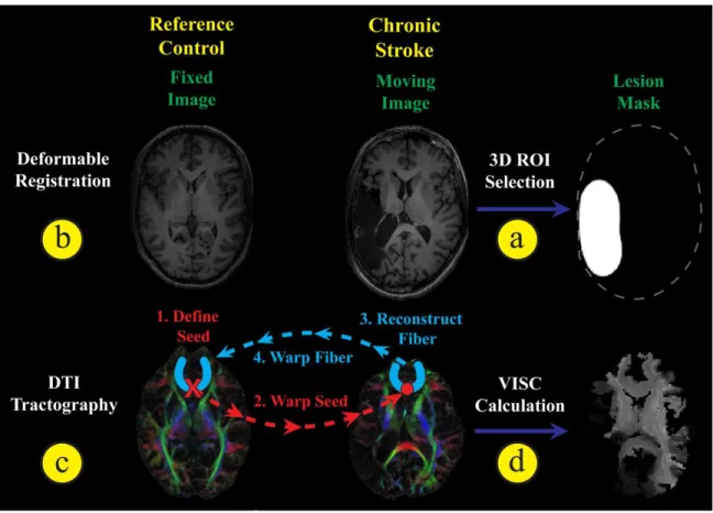
Figure 2-1: Overview diagram of image processing.
Overview of image registration, DTI tractography, and VISC calculation. (a) A lesion mask was manually selected from the stroke subject’s SPGR image, and then (b) the stroke subject was registered to the reference control subject. (c) The registration transform was used to warp seeds from the reference control space to perform DTI tractography in the stroke subject’s space. Reconstructed fibers were then transformed back into the reference control space and (d) used to perform structural connectivity analysis. Furthermore, a novel voxel-wise indirect structural connectivity (VISC) metric was calculated.
2.2.2.2.1 Stroke Lesion Selection and Correction
Initial registration results for stroke subjects were determined unacceptable based
on visual observation. In particular, areas in the control image were mapped to the lesion
boundary of the stroke subject. Lesion masking and a modified smoothness constraint
were introduced to preserve anatomical features near the lesion boundary (Fig 2-2). A
Although some lesions were discontinuous in some slices, they were not broken up
volumetrically. Only one contiguous unilateral lesion was selected for each subject.
During the registration, displacements that mapped the fixed image to locations inside the
lesion mask region were not updated. An edge-preserving Gaussian filter was used to
impose piece-wise continuity. This modified filtering allowed tissue surrounding the
lesion to register, while preserving the lesion features.
2.2.2.2.2 Inverse Deformation Estimate
Aside from challenges with stroke lesion mapping, the deformable registration
was performed in a small deformations setting, which led to a non-invertible deformation
field. However, an inverse transform was needed for our subsequent tractography
approach. We mitigated this problem by approximating an inverse with the following
method. First, a 3D displacement field was initialized to zero at each location. The
forward transform was used to map each physical coordinate in the fixed subject image
space to a location in the reference (control) image space. The displacement of the
inverse transform at this location was forced to map back to the fixed image coordinate.
Since this update step resulted in inhomogeneous mappings in the fixed image space, the
inverse transform was smoothed with a 2 mm full-width half-max Gaussian filter. The
update and smoothing steps were repeated for 10 iterations. This iteration number was
chosen heuristically to balance the tradeoff between computation time and residual error.
The mean and standard deviation of the final error magnitude across subjects was 0.5622
subject and the reference control based on the anatomical (T1 weighted) images. These
transformations were subsequently used for the diffusion image data.
2.2.2.2.4 Diffusion to Anatomical MRI
In order to use the anatomical image transformations for aligning the subjects in DTI space, each subject’s T1-weighted image was registered to his or her FA image. The
SPGR and FA images were histogram-matched, and then a nine-parameter 3-dimensional
affine transformation was optimized using a gradient descent algorithm with a mean
squared difference cost function.
2.2.2.3. Tractography and Voxel-wise Indirect Structural Connectivity Metric
2.2.2.3.1 DTI Tractography
Our in-house software, TFIRE, was also used for DTI tractography (Fig 2-1c) and
structural connectivity analysis (Fig 2-1d). We chose to define of a voxel by the location
of its center. This convention allowed for a straight-forward one-to-one mapping
between a connectivity matrix and an image space. Further detail is provided in the
Appendix.
Using the reference control DTI image, tractography was initialized by seeding
with uniform 1 mm spacing in all areas with an FA above 0.3. The coordinate of each
seed was transformed from control into subject space. The FACT method (Mori et al.,
1999) was implemented in TFIRE and used to reconstruct fiber trajectories seeded at
integrated using a 4th order Runge-Kutta technique with a step size of 0.1 mm. A
maximum angle of curvature of 60 degrees was used to terminate propagation at voxels
with crossing white matter fiber bundles. Since the endpoints of fibers often converge at
gray matter voxels, a minimum FA stopping criterion of 0.15 was used to allow the fibers
to propagate into the gray matter. Including white matter voxels in the VISC calculation
was intended to account for bifurcating and converging fiber pathways. After
construction was completed, all fibers with length < 1 cm or > 14 cm were excluded.
Each reconstructed white matter fiber was transformed back into the reference control
space using the inverse registration transform.
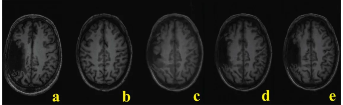
Figure 2-2: Stroke image registration.
In registering a stroke brain (a) to the template control (b), the original deformation algorithm (c) was modified to include lesion masking (d) and anisotropic smoothing (e) to produce the best result.
2.2.2.3.2 Theoretical Framework
In order to model the effects of a stroke lesion at the voxel-level, a measure of
voxel-wise indirect structural connectivity (VISC) was developed. The desired properties
connectivity of the entire brain, and to intrinsically measure these effects at the
voxel-level. We started by defining the structural connectivity of the whole brain based on the
voxel-wise direct and indirect connections obtained from DTI tractography (Fig 2-3). As
an example, consider an axonal fiber pathway that structurally connects three voxels; A,
B, and C in Figure 2-3. We defined B and C to be direct neighbors to A by their
structural connection. There are also axonal pathways that connect B or C to voxels other
than A. These pathways indirectly connect A to voxels D, E, and F, which we define as
indirect neighbors of voxel A. A connectivity graph for this example is shown in Figure
2-3b. The VISC of voxel A is the average number of connections to indirect neighbors D,
E, and F. Since F has one direct connection, and D and E each have two direct
connections, the VISC of A is 5/3.
2.2.2.3.3 Voxel-wise Indirect Structural Connectivity (VISC) Calculation
As a foundation for deriving a voxel-wise connectivity metric, the reconstructed fiber trajectories were expressed as sets of coordinates in the template control subject’s
DTI image-space. Binary matrix X represents the direct connectivity between the voxels penetrated by one reconstructed fiber, where xij is 1 if the ith and jth voxels are
both penetrated by that fiber and 0 otherwise. Matrix X represents the direct
connectivity between all voxels in an image, where xij is 1 if the ith and jth voxels are
both penetrated by at least one fiber and 0 otherwise. Thus, X is the union of individual
X across all fibers. Directly calculated from X, matrix Y represents the indirect connectivity between all voxels in an image, where yij is 1 if the ith and jth voxels share a
directly connected voxel but are not directly connected to one another. Then row vector
( )i
y from Y represents the indirect connections of the ith voxel. Using
1
as the summation vector, the VISC of the ith voxel in an image is its total number of directconnections to its indirect neighbors (expressed as y X1( )i ) divided by its total number of
indirect neighbors (expressed as y 1( )i ).
( ) ( ) VISC N N ij jk j k i i N i ij j y x y
y X1 y 1 (Eq. 1)Previously introduced voxel-wise metrics based on DTI tractography, such as
fiber count and mean fiber length (Roberts et al., 2005), are correlated with FA. In order
to consider whether fiber count information affected the correlation of VISC with FA, we
incorporated a connection count weighting factor α. This contrast mechanism gives weight to the total number of connections to a voxel’s indirect neighbors. As α is
decreased from 1 to 0, the VISC approximates the total number rather than the mean
number of direct connections to a voxel’s indirect neighbors, with VISC parameterized
by α as ( ) ( ) VISC( ) ( ) i i i y X1 y 1 . (Eq. 2)
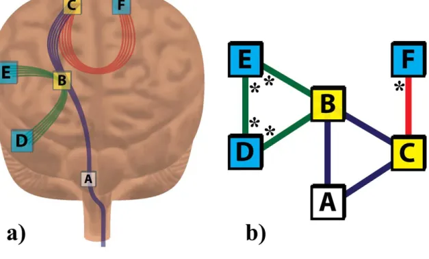
Figure 2-3: Example calculation for VISC.
The “anatomical” diagram (a) and the theoretically equivalent network graph (b)
provide the information necessary to calculate the VISC of voxel A. Voxels B and C
(yellow) are directly connected to voxel A by at least one common fiber. Voxels D, E,
and F (aqua) are indirect neighbors to voxel A because they are not directly connected to
A by any fiber but do share a common direct neighbor (B or C) with A. The VISC of
voxel A is the average number of direct connections to its indirect neighbors. These
direct connections are marked with an * in (b). Since there are 5 total direct connections