www.elsevier.com/locate/peva
Power-law vs exponential queueing in a network traffic model
Konstantinos P. Tsoukatos
a,∗,
Armand M. Makowski
baDepartment of Communications and Computer Engineering, University of Thessaly, Gklavani 37, Volos 38221, Greece bDepartment of Electrical and Computer Engineering and Institute for Systems Research, University of Maryland, College Park, MD 20742,
United States
Received 28 March 2005; received in revised form 8 January 2007 Available online 11 February 2007
Abstract
We examine the impact of network traffic dependencies on queueing performance in the context of a popular stochastic model, namely the infinite capacity discrete-time queue with deterministic service rate andM|G|∞arrival process. We propose approximations to the stationary queue size distribution which are generated by interpolating between heavy and light traffic extremes. This is done under both long- and short-range dependent network traffic. Under long-range dependence, the heavy traffic results can be expressed in terms of Mittag–Leffler special functions which generalize the exponential distribution and yet display power-law decay. Numerical results from exact expressions (when available), approximations and simulations support the following conclusions: Network traffic dependencies need to be carefully accounted for, but whether this is accomplished through a short-or long-range dependent stochastic model bears little impact on queueing perfshort-ormance. The differences between exponential and power-law queueing are negligible at the “head” of the distribution, and manifest themselves only for large buffers.
c
2007 Published by Elsevier B.V.
Keywords:Power-law queues; Mittag–Leffler function; Long-range dependence; Fractional powers; Interpolations
More than a decade of network measurement studies [24] have brought about the widespread belief that communication network traffic exhibits persistent dependencies and statistical self-similarity across a wide range of time scales. The observed dependencies are evident in sample autocorrelation functions that decay in a slower-than-exponential manner, and may often be considered non-summable. As such, they cannot be captured by Markovian models with finite exponential moments. These findings have generated a sustained interest in measuring, analyzing, simulating and forecasting network traffic, e.g., see [1] and references therein. They have also spurred intense research on the impact of high traffic variability and dependence on network performance. As a result, there is a growing body of analytical work concerning queueing models with long-range dependent inputs under a variety of scheduling disciplines [8,9,39]. When strong dependencies are present, diverse queueing patterns may arise, e.g., Weibull [12,17, 28], power-law [17,23,26] or even exponential [27]. Such conclusions mark a departure from the exponential decay commonly encountered in traditional traffic models. However, some have argued that the actual relevance of long-range dependence for network performance is questionable [21]. To complicate matters, its presence under large scale aggregations within the network core appears to be diminishing [13].
∗Corresponding author.
E-mail address:[email protected](K.P. Tsoukatos).
0166-5316/$ - see front matter c2007 Published by Elsevier B.V.
In this paper, we look into the impact of network traffic dependencies on queueing performance from a different perspective. We do so by relying on heavy and light traffic limit theorems, under both long- and short-range dependent network traffic. To the best of our knowledge, there does not seem to be prior work addressing light traffic limits under long-range dependence. We then combine asymptotic theory (through approximations) and simulation experiments in order to contrastexponentialqueueing, typically associated with short-range dependent arrivals, againstpower-law queueing, often induced by heavy-tailed traffic. At first, these dissimilar asymptotics seem to call for different buffer provisioning practices. Our work sheds some light on the actual differences between these two (apparently) vastly different queueing regimes.
The study is carried out in the context of a specific discrete-time queueing model with a deterministic service rate, a system often used as a surrogate for a multiplexer at a network node. Incoming packet traffic arrives in bursts; their durations follow an arbitrary, possibly long-tailed, distribution (or pmf)G and burst initiation epochs form a Poisson process. This family of traffic processes has come to be known asM|G|∞processes. A fluid queue fed by the continuous time version of such processes was studied earlier by Cohen [14]. Later, it was observed by Cox [15] that theM|G|∞busy server process with Pareto-tailedGis a second order asymptotically self-similar process; this important special case is also called a Poisson Pareto burst process [2]. The recent popularity of M|G|∞processes can be attributed to some measure of analytical tractability [29], and to the fact that they arise as the aggregation limit of many sporadic on/off traffic sources. From a more practical viewpoint,M|G|∞processes are attractive due to their flexibility in providing a good match to correlation functions of actual network traffic, a feature exploited in the case of VBR video modeling [25].
Our focus is on the steady-state (or stationary) queue length distribution at this network multiplexer fed by an M|G|∞ traffic process with arbitrary burst duration pmf G. When G is geometric, a two-dimensional Markov chain formulation can be developed, leading to a functional equation for the z-transform of the stationary queue length [11]. For an arbitrary pmfG, expressions for thisz-transform are available under slightly different modeling assumptions [16,37]. However, the evaluation of the stationary queue length distribution by numerical inversion techniques seems to offer little insight. The difficulties of an exact analysis can be bypassed by relying on the information gleaned from various asymptotic regimes. A promising approach consists in deriving approximations with the help of large buffer asymptotics [16,23,26,29]; these estimates are exact in the limit as the buffer level goes to infinity. Here, we follow an alternative approach and develop approximations which are anchored bylightandheavy traffic limit theorems. Such approximations become exact in the limit as the system utilization goes to zero and one, respectively.
The needed results concerning the heavy traffic regime can be found in [33,35]. When the M|G|∞process is short-range dependent, the associated limit for the queue size has an exponential distribution. Under long-range dependence, the corresponding distribution can be expressed with the help of a Mittag–Leffler special function which generalizes the exponential distribution and yet displays power-law decay. The role of Mittag–Leffler functions in the infinite variance setting is akin to the one assumed by the exponential distribution in classical queueing models with finite variance, suggesting that Mittag–Leffler special functions may serve as canonical representatives of power-law queueing. In this paper, we derive an alternative expression for the Mittag–Leffler function which is much more useful for numerical evaluations. This expression also underpins a particularly illuminating comparison with the exponential distribution, which helps illustrate the impact of the transition between short- and long-range dependent traffic where it can be most succinctly summarized, namely in the heavy traffic limit.
Next, turning to light traffic, we take advantage of the fact that theM|G|∞arrival process is obviously “Poisson driven”, so that the light traffic theory originally developed by Reiman and Simon [30] applies under an appropriate moment assumption. The light traffic limits for the queue withM|G|∞arrivals are notably different from those for the classicalM|G I|1 queue. This is a manifestation of the fact that work joins the system gradually (as is the case with M|G|∞inputs) and generates less queueing than work that arrives instantaneously. In addition, we show that under long-range dependence, fractional powers appear in light traffic; this suggests that the queue length distribution is not an analytic function of the arrival rate under long-range dependence. Approximations to the queue size distribution are generated by interpolating between the heavy and light traffic extremes. We use the approach of Fleming and Simon [20] when considering short-range dependent arrivals, and postulate heuristics for the case of long-range dependence.
We provide examples of approximations for several common pmfsG; in some cases the approximants assume a simple final form. Numerical results from exact expressions, approximations, and simulations support the following
conclusions: Network traffic dependencies need to be carefully accounted for, but whether this is achieved through a short- or long-range dependent stochastic model for the input has little quantitative impact on queueing performance. Power-law queueing, which arises as a consequence of infinite variance (or non-summable correlations), is mainly about the behavior far out in the tail. For practical purposes, the choice between a stochastic model with sufficiently large correlations and one with non-summable correlations bears no catastrophic consequences, as the sharp differences between exponential and power-law queues manifest themselves only for large buffers.
The interpolation method used here has the advantage of capturing accurately the “head” of the queue size distribution at small buffer levels. Hence, it naturally complements large deviations approximations which offer large buffer asymptotics but which may be irrelevant when failing to fit the “head” of the distribution. On the other hand, when Ghas finite exponential moments, we do not expect the heavy–light traffic approximation to be accurate for buffer levels much larger than the maximum burst length. It simply does not possess the correct decay rate — it does so only as the system utilization tends to one, i.e., in the heavy traffic limit. Surprisingly, this drawback is often absent under long-range dependence, since there are cases where the queue size distribution has power-law asymptotics with the same exponent for all traffic intensities! Then an approximation is more valuable, especially when considering that, in the presence of heavy tails, alternative estimates by means of simulation take an unreasonably long time to obtain. Yet, this approach is somewhat compromised by a lack of rigorously established light traffic limits under long-range dependence. Here, we rely on a postulated fractional expansion in Section5.2, but the problem is still unresolved.
The paper is organized as follows: The system model is presented in Section1. Section2 summarizes the main conclusions from the heavy traffic analysis developed in [35]; this section also discusses a useful relationship between Mittag–Leffler special functions and exponential distributions. In Section3we introduce an auxiliary queueing system with instantaneous inputs; in one important special case this system allows us to develop exact analytical expressions for the original system withM|G|∞inputs. In Section4, the light traffic expansions are developed under both long-and short-range dependent arrivals. These asymptotic results in both light long-and heavy traffic regimes are then combined into an approximation which is presented in Section5. In Section 6 we discuss various examples with particular emphasis on the accuracy of the approximations against simulations. Several proofs are given inAppendixfor sake of completeness.
1. The system model withM|G|∞arrival processes
We introduce the queueing model of interest, together with the needed notation. We start by presenting the class of M|G|∞arrival processes and some of its properties; additional facts can be found in [15,29].
Consider an infinite population of information sources operating synchronously in discrete-time as follows. Time is organized in contiguous slots of equal duration. During such a slot, a source can be in one of two states, active or idle. Information is organized into packets of equal size, and while active, a source generates information at a constant rate of one packet per time slot. When its activity period ends, a source switches off permanently, never to generate packets again.
More formally, for eachn = 0,1, . . ., letβn+1 denote the number of new sources which become active during the time slot[n,n+1). Source j, j =1, . . . , βn+1, begins generating information by the start of slot[n+1,n+2) and its activity period has durationσn+1,j (expressed in time slots). Letbn denote the number of active sources, or equivalently, the number of packets generated by the active sources, at the beginning of time slot[n,n+1). If initially (i.e., at timen =0) there were alreadybactive sources, letσ0,j denote the residual activity duration (in time slots) for the jth active source, j=1, . . . ,b.
The following assumptions are enforced throughout on the N-valued rvsb,{βn+1, n = 0,1, . . .},{σn,j, n = 1,2, . . .;j =1,2, . . .}and{σ0,j, j =1,2, . . .}: (i) These rvs are mutually independent; (ii) The rvs{βn+1, n =
0,1, . . .}arei.i.d.Poisson rvs with parameterλ >0; (iii) The rvs{σn,j, n =1, . . .;j =1,2, . . .}arei.i.d.rvs with common pmfGon{1,2, . . .}. Withσ denoting a genericN-valued rv distributed according to the pmfG, we always assumeE[σ]<∞; (iv) The rvs{σ0,j, j =1,2, . . .}arei.i.d.N-valued rvs distributed according to theequilibrium
pmfGeassociated withG, i.e., ifσedenotes a genericN-valued rv distributed according to the pmfGe, then
P[σe=n]= P [σ ≥n]
E[σ] ,
In summary, the process{bn, n = 0,1, . . .}results from “discrete-time Poisson arrivals” of information bursts with burst duration distributed according to the pmfGand with packet generation rate set at one packet/slot during the activity period of a burst — we refer toλas the burst arrival rate. Under the enforced assumptions, the sequence
{bn, n =0,1, . . .}can be identified as thestationaryversion of the busy server process of a discrete-timeM|G|∞
queue. For this reason, it is customary to refer to this packet arrival process{bn, n = 0,1, . . .}as the (stationary) M|G|∞arrival process(λ,G)(or equivalently,(λ, σ )).
As shown in [29], the correlation structure of the dependent rvs{bn, n =0,1, . . .}is controlled by the pmfGof σ. In particular, it is well known that
∞
X j=0
|cov(bn+j,bn)| = λ
2E[σ (σ+1)]
so that{bn, n=0,1, . . .}is short-range (resp. long-range) dependent if and only ifEσ2
is finite (resp. infinite). We feed this M|G|∞ arrival stream {bn, n = 0,1, . . .} into a discrete-time multiplexer with infinite buffer capacity. Letqn denote the number of packets remaining in the multiplexer buffer by the end of slot[n−1,n). If the multiplexer output link transmits at the rate ofcpackets/slot, then the buffer content sequence{qn, n =0,1, . . .}
evolves according to the Lindley recursion
q0=0; qn+1= [qn+bn+1−c]+, n =0,1, . . . . (2)
The average input rate to the multiplexer isE[bn] = λE[σ], and the system isstableif the system utilization
ρ := λE[σ]/csatisfiesρ < 1. More specifically, we haveqnH⇒nq∞for some R+-valued rvq∞ known as the
stationaryqueue size.
We are interested in evaluating the probabilityP(b, λ)that the stationary buffer contentq∞exceeds levelbwhen the burst arrival rate isλ, namely
P(b, λ):=Pλ[q∞>b], b≥0. (3)
Here, and elsewhere in the paper, we use the notationPλto emphasize the fact that theM|G|∞input process(λ,G) (together with related quantities to be introduced shortly) is parametrized byλ.
In what follows, we focus on obtaining explicit expressions for P(b, λ)in two asymptotic regimes, namely the heavy traffic limit (i.e., asλ→c/E[σ] from below) [38] and the light traffic limit (i.e., asλ→0) [30]. When doing so, it is understood that bothcandσ (or equivalentlyG) are held fixed whileλis allowed to vary to its appropriate limit withλ→c/E[σ] from below andλ→0, respectively.
2. Heavy traffic limits and Mittag–Leffler functions
We start with results on the heavy traffic behavior of the queue withM|G|∞arrivals. We tacitly assume that the heavy traffic limit of the stationary distribution is given by the stationary regime of the heavy trafficdiffusionlimit; see the references [34–36] for a similar approach and the recent paper [3] for a formal validation of this equivalence in a setting related to the one discussed here.
Throughout, for eachν >0, the Mittag–Leffler special functionEν :R→Ris defined [18, p. 206] by Eν(x):= ∞ X n=0 xn Γ(νn+1), x∈R (4)
with the Gamma functionΓ :(0,∞)→R+given by Γ(p)=
Z ∞
0
xp−1e−xdx, p>0.
With 0< ν <1, classical asymptotics for Mittag–Leffler functions [18, p. 207] imply Eν(−x)∼ 1
Γ(1−ν)·
1
In principle, the distribution of the stationary rvq∞depends jointly, and in a complicated manner, on the triplet λ,Gandc, and not just on the utilizationρ. Yet, the relevant facts from Theorems 6.1 and 6.3 of [35, p. 113] given below inProposition 1are expressed solely in terms of the utilizationρ. This practice should not create any confusion since by virtue of the convention introduced earlier,ρ → 1 is understood to meanλ→ c/E[σ] from below, while
bothcandσare held fixed.
Proposition 1. The heavy traffic limits of the stationary queue length distribution associated with the Lindley recursion(2)can be classified as follows:
(a)If Eσ2<∞ , then lim ρ→1P x 1−ρ, λ =exp −2E[σ] Eσ2 x ! , x≥0. (6)
(b)If σis distributed according to the Pareto distribution
P[σ >n]=n−α, n=1,2, . . . (7)
for some1< α <2, then lim ρ→1P x(1−ρ)−1/(α−1), λ =Eα−1 −(α−1)E[σ] Γ(2−α) x α−1 , x≥0. (8)
Part (a) ofProposition 1addresses the classical short-range dependent case, for which the heavy traffic normalizer is(1−ρ)and the limiting heavy traffic distribution is exponential. Part (b) deals with a long-range dependentM|G|∞
traffic process sinceEσ2= ∞under(7), and the heavy traffic queue length distribution is now expressed through
a Mittag–Leffler special function with power-law decay. This decay is a simple consequence of(5)(withν=α−1) which yields Eα−1 −(α−1)E[σ] Γ(2−α) x α−1∼ 1 (α−1)E[σ] · 1 xα−1 (x→ ∞). (9)
Part (b) was stated for a Pareto distribution with a specific tail, in order to make the power-law form(1−ρ)1/(α−1)
of the heavy traffic normalizer immediately apparent. However, we refer the reader to [35, p. 113] for corresponding results whenσ is distributed according to a general regularly varying distribution.
The Mittag–Leffler functions can be viewed as generalizing the exponential function (which is obtained by setting ν = 1 in (4)). We now introduce an alternative expression for the Mittag–Leffler functions [33] which makes the connection with exponential functions much more apparent. This representation has its origin in Bernstein’s characterization of Laplace transforms of probability distributions as completely monotonefunctions on R+ [19, Thm. 1, p. 439]: For 0 < ν <1, it is known [18, p. 207] that the functionx → Eν(−x)is completely monotone on
R+, i.e., for alln=0,1, . . ., we have (−1)n d
n
dxnEν(−x)≥0, x≥0.
The functionx → xν having a completely monotone derivative, a well-known composition result [19,Criterion 2, p. 441] implies that the functionx → Eν(−xν)is itself completely monotone onR+, hence is the Laplace–Stieltjes transform of some distribution and can be viewed as a mixture of exponential distributions [19, p. 439]. The precise sense in which this holds is now given.
Proposition 2. For0< ν <1, the functionR+→R:x→Eν(−xν)admits the representation Eν(−xν)=
Z ∞
0
e−x yfν(y)dy, x≥0 (10)
as a mixture of exponentials with mixing density given by fν(y)= sin(νπ)
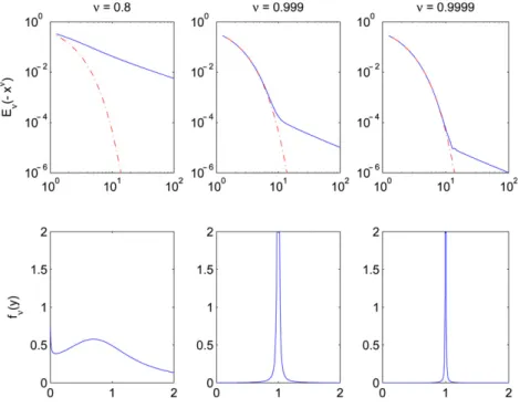
Fig. 1. Mittag–Leffler distributionsEν(−xν)and spectral densities fν(y).
The change of variablesy=(tanθ)1/νin(10)and(11)readily yields the equivalent representation Eν(−xν)= sin(νπ) νπ Z π/2 0 e−x(tanθ)1/ν 1+sin(2θ)cos(νπ)dθ, x≥0. (12)
This last expression involves an integral over a bounded interval, and is therefore more convenient for carrying out numerical calculations (as is done in Section6).
When 0< ν <1, the expression(11)yields limy↓0 fν(y)= ∞, thereby precluding thatEν(−xν)contains a single dominant exponential with strictly positive parameter. This infinite mixture of exponentials is to be contrasted with the heavy traffic queue size distribution under short-range dependence, classically given by a single exponential, the one to which expression(10)collapses asν →1 (as can be seen from the original representation(4)).
InFig. 1we illustrate the representation(10)and the convergence to the exponential distribution asν → 1. The bottom plots show the density function fν(y)forν =0.8, 0.999 and 0.9999, while the top log–log scale plots show the corresponding functionEν(−xν). The dash–dotted line depicts the negative exponential e−x. Asν→1, it is clear that the density fν(y)tends to place all of its mass aty =1, i.e., at a single exponential, a fact which also becomes apparent from the top plot for ν = 0.9999. In addition, forν = 0.9999, we observe that e−x and Eν(−xν)are very close for small values of the argumentx, yet their respective exponential and power-law tails remain strikingly different asx grows unboundedly large. We interpretFig. 1as roughly saying that “when crossing from a large, yet finite variance, to an infinite variance model, the transition in the queue length distribution occurs far out in the tail!”
3. An auxiliary system and the emptiness probability
In order to derive light traffic limits for the distribution of the stationary queue sizeq∞, we find it useful to consider a related system withinstantaneousinputs where each burst brings its entire workload into the system during asingle time slot, immediately upon arrival. These inputs are to be contrasted with the gradualM|G|∞inputs where incoming work from a burst is spread over the entire duration of the burst. Such instantaneous arrivals are represented by the sequence ofN-valued i.i.d. rvs{un,n =0,1, . . .}given by
un+1:=
βn+1 X
i=1
where the mutually independent families of i.i.d. rvs{βn+1,n =0,1, . . .}and{σn+1,i,n = 0,1, . . . ,i =1,2, . . .}
are as introduced in Section1. These arrivals are also characterized by the pair(λ,G)and letudenote the generic rv for the i.i.d. sequence{un,n=0,1, . . .}.
The instantaneous inputs{un,n=0,1, . . .}are offered to the same multiplexer with constant release ratec. With the queue initially empty, the Lindley recursion for the corresponding queue length sequence{qn(u),n =0,1, . . .}is simply
q0(u)=0; qn(u+1) = [qn(u)+un+1−c]+, n =0,1, . . . . (14) IfE[u]=λE[σ]<c, standard results for theG I|G I|1 queue [4, Cor. 6.4, p. 94] imply system stability in the sense
thatqn(u)H⇒nq∞(u)for someR+-valued rvq∞(u).
Owing to the independence of the rvs{un,n =0,1, . . .}, the recursion(14)can, at least in principle, be handled by standard generating function techniques. When the multiplexer release rate isc=1, it is straightforward to show by this method [33, Section 2.3.2, p. 24] that
Pλ h
q∞(u)=0
i
=(1−λE[σ])eλ. (15)
Furthermore, by adapting the arguments of [31] we obtain the following fact, whose proof is also available in [33, Lemma 4.3.2, p. 92].
Proposition 3. Consider the Lindley recursions(2)and(14)with respective inputs characterized by the common pair (λ, σ). If c=1andλE[σ]<1, then Pλ[q∞=0]=Pλ h q∞(u)=0 i 1+P[β=1] P[β=0]E [min(σ,X)−1] (16) whereβ is a Poisson rv with parameterλ, and X denotes a rv which is independent of the rvσ and geometrically distributed according to
P[X >k]=P[β=0]k, k=0,1, . . . . (17)
Related results, yet for a slightly different recursion, can be found in [16,37]. Combining(15)and(16), we arrive at the desired exact expression for the probabilityPλ[q∞=0] whenc=1.
Proposition 4. Consider the Lindley recursion(2)with c=1. Under the stability conditionλE[σ]<1, it holds that Pλ[q∞=0]=(1−λE[σ])eλ 1+λ ∞ X k=1 e−λkP[σ >k] ! . (18)
4. Light traffic limits
We now turn to the system behavior in light traffic. The right-hand derivatives at λ = 0 of the queue length probabilities are evaluated by means of a methodology first developed by Reiman and Simon [30], and further refined by Blaszczyszyn [6,7]. The basic advantage of this approach is to reduce the evaluation of thenth order derivative of performance measures of interest atλ=0+to calculations under scenarios where at mostnsource bursts ever arrive into the system.
For the technique to be applicable, a moment assumption is needed onσ[7].
Assumption 1. The generic burst duration rvσ satisfiesEσmax{2,c}<∞.
The light traffic analysis is straightforward but tedious, and we summarize its conclusions in the following result which is established inAppendix A.2.
Proposition 5.Consider the Lindley recursion(2)with release rate c≥1and let b≥0. If Assumption1is satisfied, then the following statements hold:
(a)For each n=0,1, . . . ,bcc, we have ∂n
∂λnP(b,0+):=limλ↓0 ∂n
∂λnP(b, λ)=0. (19)
(b)Moreover, for c=1, we have ∂2 ∂λ2P(b,0+):=limλ↓0 ∂2 ∂λ2P(b, λ) = Eh(σ−b)+2iP[σ >b]+2E(σ− b)+2− 3E(σ− b)+ P[σ >b]+P[σ >b]2. (20)
We next seek to develop some understanding into the light traffic asymptotics whenAssumption 1fails, as would be the case ifEσ2= ∞. To that end, we develop light traffic expansions which are baseddirectlyon the closed-form
expression(18)obtained whenc=1.
Using this approach we first revisit the short-range dependent case. In the process we confirm that the leading term in the light traffic expansion ofP[q∞>0] is indeed of orderλ2, and we evaluate it explicitly.
Corollary 1 (Short-range Dependence).In the setup of Proposition4withEσ2<∞, it holds that
lim λ↓0 1 λ2Pλ[q∞>0]= 1 2(E[σ (σ −1)]+2E[σ](E[σ]−1)+1) . (21)
A proof ofCorollary 1using(18)is straightforward [33, Cor. 4.3.1, p. 94]. Note that(21)is already implied by (19)and(20)forb=0.Assumption 1here takes the formEσ2<∞, which is precisely what is needed to obtain
a finite limit in(21).
More interestingly, we can exploit(18)to collect a light traffic limit for long-range dependent inputs. Such a result could not have been obtained via the Reiman–Simon theory (at least in its present form). In particular, we turn our attention to the situation whereσhas a regularly varying tail.
Corollary 2 (Long-range Dependence).In the setup of Proposition4, with the tail of σ given by(7), it holds that lim λ↓0λ −α Pλ[q∞>0]= Γ(2−α) α−1 . (22)
The light traffic result(22)can be extended to general regularly varying distributions [33, Cor. 4.3.2, p. 95]. This will not be done here in the interest of brevity, especially given that all numerical examples will be carried out under (7).
Proof. First, we observe that ∞ X k=1 e−λkP[σ >k]= 1 e−λ−1 ∞ X k=1 e−λkP[σ =k]−e−λ ! . (23)
With the help of this relation we can manipulate terms in(18)to obtain
Pλ[q∞>0] =1−eλ(1−λE[σ]) 1−λ− λ 2 e−λ−1E[σ] (24) − λe λ e−λ−1(1−λE[σ]) ∞ X k=1 e−λkP[σ =k]−1+λE[σ] ! . (25)
As this last expression explicitly displays the Laplace–Stieltjes transform ofσ, we can now invoke a Tauberian result on the asymptotic behavior of Laplace–Stieltjes transforms at the origin. In particular, Theorem 8.1.6 in [5, p. 333] provides the asymptotics of the leading term at(25)as
∞ X k=1 e−λkP[σ =k]−1+λE[σ]∼λα Γ(2−α) α−1 (λ↓0). (26)
To handle the term at(24), we first note that
lim
λ→0
e−λ−1+λ
λα =0, 1< α <2
while straightforward calculations show that
lim λ→0 1 λα 1−eλ(1−λE[σ]) 1−λ− λ 2 e−λ−1E[σ] =0. (27)
Consequently,(24)and(25)lead to(22)with the help of(26)and(27).
The impact of the distribution of σ, and in particular of its second moment, on the light traffic asymptotics of
Pλ[q∞>0] is now more apparent. Asλ ↓0, the “busy” queue probabilityPλ[q∞>0] exhibits aλ2-decay under short-range dependence. When the tail ofσ satisfies(7), theM|G|∞process is long-range dependent and the “busy” queue probability has a slower λα-fractional power decay. This provides an example of a Poisson-driven system where the performance measure of interest is not an analytic function of the Poisson rateλ. The limit(22)prompts us to conjecture that whenc=1, under(7), this fractionalλα decay of the tail probabilityPλ[q∞>b] holds more generally forall b≥0. This conjecture remains open as at the writing of this paper.
Each active source in the M|G|∞arrival process generates one packet/slot. The conditionc=1 corresponds to the case where the amount of service in one slot is exactly equal to the amount of work generated by asingleactive source during one slot. Thus, whenc=1, a single active source already utilizes the full server capacity, and there is never any leftover capacity to simultaneously serve more than one source. On the other hand, whenc>1, the server can attend to more than one source during a time slot, resulting in a multiple service feature. An exact or approximate analysis in this regime is more difficult.
Only recently has the limitation c = 1 been successfully removed in the literature on large buffer asymptotics of queues with long-range dependent inputs. In particular, a key insight obtained by large deviations arguments for heavy tails (e.g., see [10] and references therein) is that it suffices to consider events where the minimal number of simultaneously active sources generates queueing. This insight is also helpful in the present context under short-range dependence. Exactlybcc +1 active sources indeed suffice to yield the first non-zero light traffic derivative of Proposition 5(although calculations quickly get complicated forc>1). A similar argument can also be used under long-range dependence to obtain the light traffic expansion by considering scenarios with onlybcc +1 active sources. This reasoning leads us to conjecture that the desired fractional expansion forPλ[q∞>b] is of the formλ1+bcc(α−1) forallbuffer levelsb≥0. This conjecture also remains open as at the writing of this paper.
5. Heavy–light traffic interpolations
We now rely on the results in the light and heavy traffic regimes in order to construct approximations to the buffer content distribution(3)which are valid across the entire range of stable system utilization.
5.1. The short-range dependent case
UnderAssumption 1, the probabilityPλ[q∞>b] is max{c,2}times differentiable with respect toλatλ=0, and can therefore be approximated by combining heavy traffic limits and light traffic derivatives into a Taylor series-like expansion. To this end, we enforceAssumption 1throughout Section5.1and follow the approach proposed in [20]. Its main steps are given below:
For eachρin the interval[0,1)and allx≥0, we define F(x, ρ):=Pλ[(1−ρ)q∞>x]=P x 1−ρ, λ (28) where as before it is understood thatρandλare related throughρ=λE[σ]/c, and set
F(x,1):= lim
ρ→1Pλ[(1
−ρ)q∞>x]. (29)
Fixx≥0. Assume now that for somen =1,2, . . ., the partial derivatives ofF(x, ρ)with respect toρup to ordern, are available in a neighborhood ofρ =0. For notational convenience, we write
∂i ∂ρiF(x,0+)=ρlim→0 ∂i ∂ρiF(x, ρ) , i =1, . . . ,n.
Thenth order interpolation approximationbFn(x, ρ)toF(x, ρ)is the polynomial (inρ) given by
b Fn(x, ρ):= n X i=0 ρi i! ∂i ∂ρiF(x,0+)+ F(x,1)− n X i=0 1 i! ∂i ∂ρiF(x,0+) ! ρn+1
on the range 0≤ρ ≤1. With obvious notation, we observe thatbFn(x,1)=F(x,1)and that ∂i
∂ρiFnb(x,0+)=
∂i
∂ρiF(x,0+), i=0,1, . . . ,n.
In other words, bFn(x, ρ)is precisely that unique polynomial (inρ) of degreen +1 which matches then +1 first partial derivatives ofF(x, ρ)(namely those partial derivatives of degreek=0,1, . . . ,n) atρ=0 and its heavy traffic limit. By reversing the(1−ρ)normalization in bFn(x, ρ), we generate thenth order interpolation approximation to
Pλ[q∞>b] as
Pλ[q∞>b]≈bFn((1−ρ)b, ρ). (30)
This quantity may lie outside[0,1], in which case it is obviously a poor approximation.
We rely on the results of Sections2and4to implement this approach in the present setup. UnderAssumption 1, the second momentEσ2is finite andProposition 1yields
F(x,1)= lim ρ→1exp −2E[σ] Eσ2 x ! , x≥0.
Ifc≥1, then thebccth order interpolation approximation toPλ[q∞>b] is taken to be
Pλ[q∞>b]≈bFbcc((1−ρ)b, ρ)=ρbcc+1exp − 2E[σ] Eσ2( 1−ρ)b ! . (31)
In postulating(31), although we have followed the approach outlined above, we have conveniently neglected mixed partial derivatives; see [33, p. 105] for more details. This is also done for the casec=1 discussed next.
More can be accomplished whenc=1: Part (b) ofProposition 5supplies the second partial derivative, leading to the 2nd order interpolation by means of the polynomial
b F2(x, ρ)= 1 2ρ 2(1−ρ) ∂2 ∂ρ2P(x,0+)+ρ 3exp −2E[σ] Eσ2 x ! (32) and this leads to the 2nd order interpolation
5.2. The long-range dependent case
The light traffic results ofProposition 5do not cover distributions withEσ2= ∞becauseAssumption 1is now
violated, and the interpolation approach outlined above does not apply. However, we address the case of long-range dependence by constructing a sharp approximation based on the following heuristic arguments:
Consider the Pareto distribution (7) with 1 < α < 2. SinceAssumption 1 does not hold, the expression(20) fromProposition 5yields now an infinite value. This indicates that under long-range dependence,Pλ[q∞>b] may not be an analytic function ofλatλ = 0. As argued in Section4, whenc = 1,Corollary 2strongly suggests that limλ↓0λ−αPλ[q∞>b] is the non-trivial sought-after limit for allb≥0. Thus, whenc=1, these considerations lead us to postulate the existence of the limits
lim
λ→0λ −α
Pλ[q∞>b]=K(b), b≥0 (34)
for some unknown mapping K : R+ → R+. ByCorollary 2we already have K(0)= Γ(2−α)/(α−1). On the other hand, the heavy traffic result of Proposition 1(b) hints at a possible approximation around the normalized rv (1−ρ)1/(α−1)q∞, leading us to propose the approximation
Pλ[q∞>b]≈Eα−1 −(α−1)E[σ] Γ(2−α) 1−ρ ρα bα−1 , c=1. (35)
This expression is in agreement with the heavy traffic limit(8)sinceρ−α(1−ρ)∼(1−ρ)asρ → 1. In addition, from the asymptotics(5), asb→ ∞, we also find that
Eα−1 −(α−1)E[σ] Γ(2−α) 1−ρ ρα bα−1 ∼ 1 (α−1)E[σ] · ρ α 1−ρ · 1 bα−1.
This ensures that, asρ→ 0, the approximation(35)conforms with the conjectured light traffic limit(34). However, it remains unclear what form should the higher order terms assume in the fractional expansion under long-range dependence, and whether there exists a relationship between heavy and light traffic limits that generalizes a result of Simon [32].
6. Numerical results
To quantify the impact of dependencies on queueing behavior, we collect numerical results from the proposed approximations and from simulation experiments. The accuracy of the approximations is gauged by comparing with simulation data under various choices for the distributionGof the burst duration rvσ. The experimental values are obtained by regenerative simulation [22] and the relative widths accompanying them correspond to 95% confidence intervals. We almost exclusively (with one exception) confine ourselves to the simple situation where the multiplexer release rate isc=1. While the list of examples below is not exhaustive, the discussion does illustrate the ability of the heavy–light traffic interpolation to “ballpark” the true tail probabilities, as well as its limitations. It also highlights the fact that emerging power-law queueing patterns under long-range dependence are not captured by finite variance models, but that this failure occurs only as buffers grow large.
DeterministicWhen the burst duration is deterministic, sayσ = Da.s. for some positive integer D, approximation (33)reads Pλ[q∞>b]≈ ρ 2(1−ρ) 2D2 (3[D−(1−ρ)b] +([D−(1−ρ)b]+−1) +1[D> (1−ρ)b])+ρ3exp −2 D(1−ρ)b for allb≥0.
With D =3, we obtain simulation estimates for the steady state probabilityPλ[q∞>0]. Of course, in this case the exact expression is available for b = 0 at(18). InTable 1we list simulation estimates and numerical values from(18)and from the light–heavy traffic interpolation. There is excellent agreement between the values generated through the exact formula(18)and through the light–heavy traffic interpolation. Since we expect the approximation to
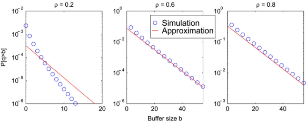
Fig. 2. Geometric burst duration withγ =2/3 and release ratec=4. Table 1
Pλ[q∞>0] for deterministic burst durationσ=3
ρ Exact Simulation Approximation Error (%)
0.1 1.0478e−02 1.0469e−02±0.2% 1.0500e−02 −0.21
0.2 4.1622e−02 4.1668e−02±0.3% 4.1778e−02 −0.38
0.3 9.3042e−02 9.3020e−02±0.2% 9.3500e−02 −0.49
0.4 1.6441e−01 1.6442e−01±0.2% 1.6533e−01 −0.56
0.5 2.5545e−01 2.5533e−01±0.2% 2.5694e−01 −0.58
0.6 3.6594e−01 3.6607e−01±0.1% 3.6800e−01 −0.56
0.7 4.9573e−01 4.9601e−01±0.1% 4.9817e−01 −0.49
0.8 6.4470e−01 6.4488e−01±0.1% 6.4711e−01 −0.37
0.9 8.1279e−01 8.1264e−01±0.1% 8.1450e−01 −0.21
be asymptotically exact at the endpointsρ=0 andρ=1, it is not surprising that the largest errors occur in moderate traffic.
GeometricIfσ follows a geometric distribution, e.g.,P[σ >n]=γn,n=0,1, . . ., with 0< γ <1, then we obtain
from(33)that Pλ[q∞>b]≈ ρ2 2 (1−ρ)(1+γ ) 2γ2(1−ρ)b+ρ3exp −21−γ 1+γ(1−ρ)b for allb≥0.
Ifc> 1, then the expression(33)is not applicable, the first non-zero light traffic derivative is not available, and the only available heavy–light traffic approximant is(31). We illustrate its behavior by means of an example where γ =2/3 andc=4. The resulting log–linear plots inFig. 2correspond to system utilizationsρ =0.2,ρ =0.6 and ρ = 0.8. The approximation fares very well in moderate to heavy loads, but obviously yields inaccurate results for ρ=0.2 due to insufficient light traffic information.
ParetoLet the burst duration rvσ follow the Pareto distribution(7) with 1 < α < 2, in which case theM|G|∞
process is long-range dependent and the approximation(35)is in effect. Assessing the performance of(35)requires a numerical evaluation of the Mittag–Leffler function, a task carried out by numerical integration with the help of the alternative expression(12).
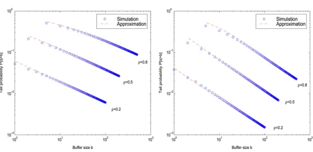
We have tested the approximation(35) for system utilizationsρ = 0.2,0.5 and 0.8, and release ratec = 1. Under long-range dependence, simulation estimates converge very slowly. Moreover confidence intervals based on the regenerative method cannot be constructed because the underlying regenerative period has infinite variance. In the results shown inFig. 3, the runs were 109time slots long, by which time the estimates had stabilized. The log–log scale plots correspond to two Pareto distributions with parametersα=1.5 andα=1.7, respectively. As expected, the heavier Pareto tail withα=1.5 induces larger tail probabilities than the Pareto tail withα=1.7, at thesamesystem utilizations. InFig. 3, simulated and approximate values are seen to be very close, suggesting that the expression
Fig. 3. Pareto burst duration withα=1.5 (left) andα=1.7.
(35)provides a satisfactory approximation. Note the almost linear shape of the curves in log–log scale, reflecting the power-law asymptotics of the queue size distribution announced in [23,26].
Truncated Pareto When σ follows a truncated Pareto distribution, the resulting M|G|∞ process is short-range dependent. Yet, over a finite range of time scales, it can display dependences similar to those of a long-range dependent M|G|∞process. Specifically, for 1< α <2, pick someN =2,3, . . .and consider the truncated Pareto distribution on{1,2, . . . ,N}given by P[σ >n]= 1 1−N−α(n −α− N−α), n=1,2, . . . ,N. (36)
The distribution(36)has finite support and clearly satisfiesAssumption 1. The integer parameterNprovides a means to control the tail behavior ofσ, hence the dependencies in theM|G|∞arrivals. When N =2, the corresponding rv σ is deterministic withσ =2 a.s. AsNincreases, the second moment of the burst duration distribution also increases, thus leading to stronger dependences in theM|G|∞process. AsN goes to infinity, the rvσ converges weakly to the standard Pareto distribution(7). As a result, we move from a rvσwith finite exponential moments to a rv with infinite variance, hence to a correspondingM|G|∞process that is long-range dependent.
To illustrate the effect of dependences in the traffic process on the resulting queue size distribution, we carry out simulation experiments withα=1.7 and for the two truncation levelsN =50 andN =1000. Results are collected for system utilizationsρ =0.2,0.5,0.8. As approximation(33)does not assume any simple closed form expression in this case, we evaluated numerically the various quantities entering(33). InFig. 4we compare simulation results for truncation level N =50 with the approximate values obtained from(33)(labeled SRD) and those from expression (35)(labeled LRD). Confidence intervals widths are not shown since, with the exception of the three points at the bottom of the plot, they were well within 10% of the mean. The curves corresponding toρ=0.2,0.5 and 0.8, show that the SRD approximation tracks the true queue size probabilities satisfactorily, especially for small buffer sizes. As the target probabilities become smaller and the buffer size of interest increases, it is clear that the quality of the SRD approximation degrades.
Further increase in N is expected to reveal the limitations of the SRD approximation(33). Still withα = 1.7, increasing N from 50 to 1000 results in a small increase in the expectation fromE[σ] = 2.9 to E[σ] = 3.035,
and in a large increase in the second moment fromEσ2 = 15.863 toEσ2 = 42.49. Obviously, the larger the
variance of the truncated Pareto rv, the closer the simulation curve will be to that of the LRD approximation(35). Moreover, for a fixed variance of the rvσthe match between the simulation curve and that of the LRD approximation is better at smaller buffer sizes. On the other hand, as the buffer size grows to infinity, the LRD approximation(35) will also eventually fail: It exhibits a power-law decay, while, as follows from the developments in [29], the queue size distribution induced by truncated Pareto burst durations decays exponentially fast.
Fig. 4. Exponential vs. power-law approximations; truncated Pareto bursts withα=1.7 andN=50.
Fig. 5. Simulations: Pareto vs. truncated Pareto withα=1.7 andN=1000.
This contrast between the queueing behavior of truncated Pareto with N = 1000, and standard Pareto burst durations is more evident when comparing the log–log plots of simulated values for Pareto and truncated Pareto bursts inFig. 5. Although the shape of the left part of all curves inFig. 5is almost linear, thus suggestive of a hyperbolic initial segment, the rightmost part of the truncated Pareto curves decreases rapidly and the curves turn concave, in agreement with the anticipated exponential decay. Nevertheless, in spite of the different buffer asymptotics, it is clear that all numerical values from simulations, and both LRD and SRD approximations remain close at the “head” of the distribution. Also recall that the present queueing model withc =1 exhibits the smallest possible degree of traffic aggregation, as a single active source suffices to exhaust the link capacity. Hence the effect of long range dependence is expected to remain rather pronounced. Still,Fig. 5shows that for buffer levels that are roughly up to 10, i.e., three times the average burst sizeE[σ], any infinite variance effects go virtually unnoticed. This pattern should emerge more forcefully in the casec>1; unfortunately light traffic limits are then unavailable. These observations underscore the fact that the time dependencies of theM|G|∞arrivals, namely long-range vs. short-range dependence, do not have significant quantitative impact for small buffers. The transition between exponential and power-law queueing, and the so-called ineffectiveness of buffering for long-range dependent traffic emerge as buffer sizes grow to infinity.
Fig. A.1. Integration path.
Acknowledgments
The authors would like to thank the Editor and the referees for suggestions that considerably improved the paper. The work of the first author was supported through an ARCHIMEDES grant by the Greek Ministry of Education.
Appendix
A.1. A proof ofProposition2
Fix 0< ν <1. From [18, Eq. (18) p. 209] (or [33, Eq. (3.20) and (3.23) p. 43]), we collect the Laplace transform pair Z ∞ 0 e−s xEν(−xν)dx= 1 s 1 1+s−ν, s≥0. (A.1)
A representation of the form(10)is obtained forEν(−xν)by using the definition of the Laplace inversion integral Eν(−xν)= lim L→∞ 1 2πj Z d+j L d−j L es x1 s 1 1+s−νds, x≥0 (A.2)
where we pickd to be any strictly positive abscissa on the real axis. To evaluate(A.2), we note that the denominator 1+s−νhas roots of the formsm=e−j
2m+1
ν π for allm=0,±1, . . .. Since 0< ν <1, we have|2mν+1| >1 for every m=0,±1, . . ., so that there is no root with argument in[−π, π]. Thus, by standard arguments, the integral(A.2)can be evaluated along the clockwise path fromHtoAshown inFig. A.1through
Eν(−xν)= lim R→∞ r→0 1 2πj Z A H es x1 s 1 1+s−νds, x ≥0. (A.3)
In the limit, as the radiusR goes to infinity, the contributions of the arcsC BandG Fto the integral above are zero by Jordan’s lemma. The limiting contributions of the arcs H GandB Aare also zero, because their length is bounded and es x is also bounded along these arcs. Finally, on the circular arcE Dwe sets=rejφ,φin[−π, π], and see that the resulting integrand vanishes asr → 0. Thus, in(A.3)only the integrals along the segmentsF E andDC remain in the limit. Settings=ye−jπ ands=yejπ,y>0, forF E andDC, respectively, we collect
Eν(−xν)= 1 2πj Z ∞ 0 e−x y1 y 1 1+yνe−jνπ − 1 1+yνejνπ dy, x≥0 and manipulating we readily arrive at(10)with density(11).
Fig. A.2. Queue length evolution under the event{t1,t2;k1,k2}.
A.2. A proof ofProposition5
A proof of Part (a) can be found in the thesis [33] and is omitted as it proceeds along the same lines as the proof of Part (b) which we now provide. We apply the methodology outlined in [7,30]; see [33] for additional details. With the functionalψ taken to beψ := 1[q0>b] for someb ≥ 0, we see that the performance measure of interest is φ(λ)= Eλ[ψ]=Pλ[q∞>b], i.e., the probability that the queue content exceeds levelb. From the developments in [7,30] we get d2 dλ2φ(0+)=E e ψ(σ1, σ2) (A.4) whereσ1andσ2are i.i.d. copies of the generic activity duration rvσ andψeis defined by
e ψ(k1,k2):= +∞ X t1=−∞ +∞ X t2=−∞ ψ({t1,t2;k1,k2}) (A.5)
for allk1,k2=0,1, . . ., where for allt1,t2=0,±1,±2, . . ., we write ψ({t1,t2;k1,k2}):=1[q0>b]({t1,t2;k1,k2})
for the indicator function that the queue length at timet =0 exceedsb, conditioned on the event{t1,t2;k1,k2}where only two source bursts ever join the system, in slots[t1−1,t1)and[t2−1,t2), with activity durationsk1 andk2, respectively.
We thus need only examine the queue length process induced by events of the form{t1,t2;k1,k2}. If
min(t2+k2,t1+k1) >max(t1,t2), (A.6)
the two sources arriving in slots[t1−1,t1)and[t2−1,t2)are simultaneously active from time max(t1,t2)until min(t2+k2,t1+k1). In that case the queue size evolves as shown inFig. A.2. Otherwise, i.e., if min(t2+k2,t1+k1)≤ max(t1,t2), the queue size is identically zero. By inspection, under(A.6), the queue lengthq0({t1,t2;k1,k2})at time
t=0 is given by
−max(t1,t2) if max(t1,t2)≤0 and 0≤min(t1+k1,t2+k2)
min(t1+k1,t2+k2)−max(t1,t2) if min(t1+k1,t2+k2) <0 and 0≤max(t1+k1,t2+k2) min(t1,t2)+k1+k2 if max(t1+k1,t2+k2) <0 and 0≤min(t1,t2)+k1+k2
Fig. A.3. Values of1
q0>b({t1,t2;k1,k2})fork1<k2.
By symmetry we need only calculateψefork1<k2. Clearly, in order forq0to be greater thanb, it is necessary that
k1>b. If this is not true, i.e. ifk1≤b, then1[q0>b]=0, henceψecorresponding toψ :=1[q0>b] is also zero and(20)follows via(A.5)and(A.4). Now, ifk1 >bthen thet1t2-plane does indeed contain a region whereψ =1. We showψ({t1,t2;k1,k2})corresponding toψ :=1[q0>b] and identify this region inFig. A.3. Using this graph, calculation ofψ(ek1,k2)from the double sum(A.5)is a matter of algebra. From the points along the linet1 = −k1, which splits theψ=1 region in two trapezoids, we collect
−b−1
X
i=−(k1+k2)+b+1
1=k1+k2−2b−1 (A.7)
while on the right trapezoid the double sum can be calculated as k2−b−2 X j=0 (j+k1−b)= 1 2(2k1+k2−3b−2)(k2−b−1). (A.8)
On the left trapezoid we find k1−b−2 X j=0 (k1+k2−2b−2−j)= 1 2(2k2+k1−3b−2)(k1−b−1). (A.9)
Collecting the expressions(A.7)–(A.9), and inserting back into(A.4)and(A.5), we readily conclude to(20).
References
[1] P. Abry, R. Baraniuk, P. Flandrin, R. Riedi, D. Veitch, The multiscale nature of network traffic, IEEE Signal Processing Magazine 19 (3) (2002) 28–46.
[2] R.G. Addie, T.D. Neame, M. Zukerman, Performance evaluation of a queue fed by a Poisson Pareto burst process, Computer Networks 40 (3) (2002) 377–397.
[3] J. Alvarez, B. Hajek, A queue with semi-periodic traffic, Advances in Applied Probability 37 (1) (2005) 160–184. [4] S. Asmussen, Applied Probability and Queues, second ed., Springer-Verlag, New York, NY, 2003.
[5] N.H. Bingham, C.M. Goldie, J.T. Teugels, Regular Variation, in: Encyclopedia of Mathematics and its Applications, Cambridge University Press, Cambridge, UK, 1987.
[6] B. Blaszczyszyn, Factorial-moment expansion for stochastic systems, Stochastic Processes and their Applications 56 (1995) 321–335. [7] B. Blaszczyszyn, Factorial moment expansion for functionals of point processes with application to approximations of stochastic models,
[8] S. Borst, O.J. Boxma, R. Nunez-Queija, A.P. Zwart, The impact of service discipline on delay asymptotics, Performance Evaluation 54 (2) (2003) 175–206.
[9] S. Borst, M. Mandjes, M. van Uitert, Generalized processor sharing with light-tailed and heavy-tailed input, IEEE/ACM Transactions on Networking 11 (5) (2003) 821–834.
[10] S. Borst, B. Zwart, Fluid queues with heavy-tailedM/G/∞input, Mathematics of Operations Research 30 (4) (2005) 852–879.
[11] A. Brandt, M. Brandt, H. Sulanke, A single server model for packetwise transmission of messages, Queueing Systems. Theory and Applications 6 (1990) 287–310.
[12] F. Brichet, J. Roberts, A. Simonian, D. Veitch, Heavy traffic analysis of a storage model with long range dependent on/off sources, Queueing Systems. Theory and Applications 23 (1996) 197–215.
[13] J. Cao, W. Cleveland, D. Lin, D. Sun, Internet traffic tends to Poisson and independent as the load increases, Technical Report, Bell Labs, 2001.
[14] J.W. Cohen, Superimposed renewal processes and storage with gradual input, Stochastic Processes and their Applications 2 (1974) 31–58. [15] D.R. Cox, Long-range dependence: A review, in: H.A. David, H.T. David (Eds.), Statistics: An Appraisal, Iowa State University Press, Ames,
IA, 1984, pp. 55–74.
[16] T. Daniels, C. Blondia, Asymptotic behavior of a discrete-time queue with long-range dependent input, in: Proceedings of the IEEE Infocom’99, New York, NY, 1999.
[17] N.G. Duffield, N. O’Connell, Large deviations and overflow probabilities for the general single server queue, with applications, in: Mathematical Proceedings of the Cambridge Philosophical Society, vol. 118, 1995, pp. 363–374.
[18] A. Erd´elyi, Higher Transcendental Functions, vol. 3, McGraw-Hill, New York, NY, 1955.
[19] W. Feller, An Introduction to Probability Theory and its Applications, vol. II, John Wiley and Sons, New York, NY, 1972. [20] P.J. Fleming, B. Simon, Interpolation approximations of sojourn time distributions, Operations Research 39 (2) (1991) 251–260.
[21] M. Grossglauser, J.-C. Bolot, On the relevance of long-range dependence in network traffic, IEEE/ACM Transactions on Networking 7 (5) (1999) 629–640.
[22] R.K. Jain, The Art of Computer Systems Performance Analysis: Techniques for Experimental Design, Measurement, Simulation, and Modeling, Wiley, 1991.
[23] P.R. Jelenkovi´c, A.A. Lazar, Asymptotic results for multiplexing subexponential on-off processes, Advances in Applied Probability 31 (2) (1999) 394–421.
[24] T. Karagiannis, M. Molle, M. Faloutsos, Long range dependence: Ten years of Internet traffic modeling, IEEE Internet Computing 8 (2004) 57–64.
[25] M.M. Krunz, A.M. Makowski, Modeling video traffic usingM|G|∞input processes: A compromise between Markovian and LRD models, IEEE Journal on Selected Areas in Communications 16 (5) (1998) 733–748.
[26] Z. Liu, Ph. Nain, D. Towsley, Z.-L. Zhang, Asymptotic behavior of a multiplexer fed by a long-range dependent process, Journal of Applied Probability 1 (36) (1999) 105–118.
[27] A.M. Makowski, Long–range dependence does not necessarily imply non-exponential tails, IEEE Communications Letters 6 (12) (2002) 550–552.
[28] I. Norros, A storage model with self-similar input, Queueing Systems. Theory and Applications 16 (1994) 387–396.
[29] M. Parulekar, A.M. Makowski, Tail probabilities for M|G|∞processes (I): Preliminary asymptotics, Queueing Systems. Theory and Applications 27 (1997) 271–296.
[30] M.I. Reiman, B. Simon, Open queueing systems in light traffic, Mathematics of Operations Research 14 (1989) 26–59.
[31] K. Sigman, G. Yamazaki, Fluid models with burst arrivals: A sample path analysis, Probability in the Engineering and Informational Sciences 6 (1992) 17–27.
[32] B. Simon, A simple relationship between heavy and light traffic limits, Operations Research 40 (1992) S342–S345.
[33] K.P. Tsoukatos, Heavy and light traffic regimes forM|G|∞traffic models, Ph.D. Thesis, University of Maryland, College Park, MD, May 1999.http://techreports.isr.umd.edu/reports/1999/PhD 99-6.pdf.
[34] K.P. Tsoukatos, A.M. Makowski, Heavy traffic analysis for a multiplexer driven byM|G I|∞input processes, in: Proceedings of the 15th International Teletraffic Congress, Washington, D.C., June 1997, pp. 497–506.
[35] K.P. Tsoukatos, A.M. Makowski, Heavy traffic limits associated withM|G|∞input processes, Queueing Systems. Theory and Applications 34 (1–4) (2000) 101–130.
[36] K.P. Tsoukatos, A.M. Makowski, Asymptotic optimality of the Round–Robin policy in multipath routing with resequencing, Queueing Systems. Theory and Applications 52 (3) (2006) 199–214.
[37] S. Wittevrongel, H. Bruneel, Correlation effects in ATM queues due to data format conversions, Performance Evaluation 32 (1–4) (1998) 35–56.
[38] W. Whitt, Stochastic-Process Limits: An Introduction to Stochastic-Process Limits and their Applications to Queues, Springer-Verlag, New York, NY, 2002.
[39] A. Zwart, O.J. Boxma, Sojourn time asymptotics in theM|G|1 processor sharing queue, Queueing Systems. Theory and Applications 35 (1–4) (2000) 141–166.
Konstantinos (Kostas) Tsoukatosreceived the Diploma degree from the National Technical University of Athens, Greece in 1992, a M.Sc. and a Ph.D. in Electrical Engineering from the University of Maryland, College Park, in 1994 and 1999 respectively. He was a recipient of an Eugenides Foundation Scholarship for graduate studies in the United States in 1993, and a summer intern at the IBM T.J. Watson Research Center, NY, in 1994 and 1995. During 2000–2001 he was a research associate with the Telecommunications Laboratory, National Technical University of Athens. Since February 2003 he is as an adjunct assistant professor at the Communications and Computer Engineering Department, University of Thessaly, Volos. His interests are in performance modeling of wireless and wireline networks; topics include queueing analysis of self-similar Internet traffic, optimal scheduling in parallel systems, and resource allocation in wireless.
Armand M. Makowskireceived the Licence en Sciences Math´ematiques from the Universit´e Libre de Bruxelles in 1975, the M.S. degree in Engineering-Systems Science from U.C.L.A. in 1976 and the Ph.D. degree in Applied Mathematics from the University of Kentucky in 1981. In August 1981, he joined the faculty of the Electrical Engineering Department at the University of Maryland College Park, where he is Professor of Electrical and Computer Engineering. He has held a joint appointment with the Institute for Systems Research since its establishment in 1985.
Armand Makowski was a C.R.B. Fellow of the Belgian-American Educational Foundation (BAEF) for the academic year 1975–76; he is also a 1984 recipient of the NSF Presidential Young Investigator Award and he became an IEEE Fellow in 2006.
His research interests lie in applying advanced methods from the theory of stochastic processes to the modeling, design and performance evaluation of engineering systems, with particularemphasis on communication systems and networks.