High Dynamic Range Video Using Split Aperture Camera

High Dynamic Range Video Using Split Aperture Camera

Hongcheng Wang

, Ramesh Raskar

, Narendra Ahuja

†

_{Beckman Institute, University of Illinois at Urbana-Champaign (}

_{), IL, USA}

_{Mitsubishi Electric Research Laboratories (}

_{), MA, USA}

Abstract

We present a new approach to display High Dynamic Range (HDR) video using gradient based high dynamic range compression. To obtain HDR video, we utilize the split aperture camera. We apply a spatio-temporal gradient based video integration algorithm for fast and accurate in-tegration of the three input HDR videos into a low dynamic range video, which is suitable for display. The spatio-temporal video integration generates videos with spatio-temporal coherency and without artifacts. In order to improve the computational speed, we propose using a diagonal multi-grid algorithm to solve the Poisson equation. We show ex-perimental results on a variety of dynamic scenes.

1

Introduction

A conventional digital camera typically provides a dy-namic range of two orders of magnitude through theCCD’s analog-to-digital converter (The ratio in intensity between the brightest pixel and the darkest pixel is usually referred to the dynamic range of a digital image). However, many real-world scenes have a larger brightness variation. Thus, some areas of the images captured by digital cameras are undersaturated or oversaturated.

Tonemapping (also called tone reproduction) is used to establish an efficient way to reconstruct faithfully the high dynamic range radiance on a low dynamic range image for display. Display of HDR video is the main problem we address in this paper. To capture a high dynamic range image, several images with different exposures are usually taken to cover the whole range of a real scene using con-ventional cameras. Those images are combined into a sin-gle high dynamic range image (radiance map). High dy-namic range radiance maps are then recovered from these images [3]. Tonemapping methods are then applied to the radiance maps to reduce the dynamic range. The resultant low dynamic range (LDR) image can be viewed on conven-tional display devices.

Capturing high dynamic range video involves dealing

with motion in the scene and hence it is not possible to capture the radiance map via a single camera with succes-sive multi-exposures. In addition, for tone mapping HDR videos, we cannot trivially tonemap successive frames of the video. This naive approach will lack temporal coherence resulting in flicker. Thus capture and compression of HDR video has remained a challenging problem. As described later, some commercial and research hardware approaches have been proposed to this problem. In one of the few soft-ware solutions presented to this problem, Kang et. al. [7] describe an approach by varying the exposure of alternate frames. It requires a burdensome registration of features in successive frames to compensate for motion. Given the feature correspondence problem, rapid movements and sig-nificant occlusions cannot be dealt with easily. In addition, the two different exposures may not capture the full radi-ance map of a scene. More exposures will make the feature registration problem more difficult.

In this paper, we propose a new approach for display-ing HDR video usdisplay-ing gradient based HDR compression ap-proach. We use a camera rig composed of three built-inCCD sensors, which share the same view on a shared optical axis. Hence, we can capture truly dynamic scenes without frame registration. Our major contribution is a new 3D integration algorithm for HDR video compression. We use diagonally oriented grids to fast and accurately obtain the solutions of the resulting Poisson’s Equation in three-dimension space.

2

Related Work

Though capturing high dynamic range video is not our main contribution, a specially designed camera is used in our HDR video display framework to overcome the disad-vantages of the work by Kang et.al’s [7]. Therefore, we first present a brief review on HDR capturing followed by the related work in tonemapping.

2.1

Capture

To capture HDR video, sequential exposure change [12, 13, 11] is not an option. Some researchers have proposed

using specially designed single sensor [2, 21, 9] or multi-ple image sensors [1, 19], as well as spatially varying [13] or spatio-temporally varying [14] pixel exposures sensors. SomeCCDsensors are designed with each pixel having two elements with different sensitivity [21, 9]. In [2], authors describe a sorting computational sensor on which each pixel can measure the time to obtain full potential well capacity. All pixels of the input image are sorted according to their intensities. Many of these techniques trade spatial resolu-tion for dynamic range while maintaining the video frame rate.

Several methods have been proposed that do not entail the above tradeoff. [14] adapts the exposure of each pixel on the image detector using a controllable attenuator based on the radiance of the corresponding scene point.

Multiple image sensors [1, 19] are often used to capture video-rate HDR video while keeping the spatial resolution of original sensors. For example, Aggarwal and Ahuja [1] use a mirror-based beam splitter to split the light refracted from the lens into three beams, which reach three different sensors. The camera has video-rate capacity and controlled exposure time for each of the sensors. We use a similar 3 channel camera in our prototype.

2.2

Display (Tonemapping)

Many tonemapping algorithms for compressing and dis-playing HDR images have been proposed [4, 5, 22, 17]. Du-rand et al. [4] propose using bilateral filtering to decompose an HDR image into a base layer and a detail layer, and then compress the contrast of the base layer. Reinhard et al. [17] achieve local luminance adaptation by using photographic technique of dodging-and-burning. Tumblin and Turk [22] propose the low curvature image simplifier LCIS by apply-ing anisotropic diffusion to prevent halo artifacts. Fattal et al. [5] propose a method to attenuate high intensity gradi-ents while magnifying low intensity gradigradi-ents. The lumi-nance is recovered from the compressed gradients by solv-ing a Poisson equation.

In spite of the great efforts onHDR IMAGEdisplay, ro-bust algorithms for tonemapping HDR VIDEO are not yet common. Kang et.al. [7] propose a solution to prevent flick-ering in the mapping due to temporal inconsistency. But only a global mapping is applied which is not adaptive to the coarse temporal intensity variations.

In this paper, we propose a gradient domain technique to compress high dynamic range videos. Our work is inspired by that of Fattal et.al. [5]. The resulting images have no halos and other artifacts. However, we can not apply the dynamic range compression method directly in a frame-by-frame manner. This is because the temporal consistency will be violated, and undesired flickering and color shift will result due to shift and scale ambiguity in image integration

and tonemapping exponents in color assignment.

3

Gradient Domain Video HDR

Compres-sion

Gradient domain techniques have been widely used in computer vision and computer graphics. The idea is to min-imize the gradient difference between the source and tar-get images when the gradient field of the source image is modified to obtain the target one. This technique is in-spired by the retinex theory originally proposed by Land and McCann in 1971 [10]. Since then a number of appli-cations based on this technique have been proposed, such as image editing [15], shadow removal [6], multispectral image fusion [20], image and video fusion for context en-hancement [16] and HDR image compression [5]. Most re-cently, we extended the gradient based technique to three-dimensions by considering both spatial and temporal gradi-ents, and applied to video editing [23]. This paper addresses a new application, HDR video compression, for split aper-ture camera.

3.1

Video as 3D Cube

The gradient domain method proposed by Fattal et.al. [5] can be considered 2D integration of modified 2D gradi-ent field. As mgradi-entioned earlier, the integration involves a scale and shift ambiguity in luminance plus an image de-pendent exponent when assigning colors. Hence, a straight-forward application to video will result in lack of temporal coherency in luminance and flicker in color. We instead treat the video as a 3D block of pixels and solve problem via 3D integration of a modified 3D gradient field.

3.2

3D Video Integration

Our video HDR compression problem is stated as fol-lows: Given n synchronized LDR videos, I1, I2, . . . , In, with different exposures, find an HDR video, I, which is suitable for typical displays. First, the radiance map from the input videos can be computed using a method such as in [3] for corresponding images in the videos (We will not discuss the details of recovering the radiance map here). Then our task is to generate a new video,I, whose gradi-ent field is closest to the gradigradi-ent of the HDR radiance map video,G. The general algorithm for HDR video display is described in Algorithm 1.

One natural way to achieve this is to solve the equation

∇I=G (1)

However, since the original gradient field is modified in some way (attenuated high gradient and magnified low gra-dient in our case), the gragra-dient field G is not necessarily

Algorithm 1: General algorithm for HDR video display Data:LDRvideoI1, I2, . . . , In

Result: HDR videoI

Recover the radiance map;

Attenuate large gradients and magnify small ones (Sec. 3.3);

Reconstruct new videoIby solving a Poisson equation;

integrable. Some part of the modified gradient may violate

∇ ×G= 0 (2) (i.e. the curl of gradient is 0). This is a special case of the formulation by Kimmel et.al. [8] in the sense that only the gradient field is considered here. Kimmel et.al. proposed minimizing a penalty function of gradient and intensity us-ing a variational framework. A projected normalized steep-est descent algorithm was proposed to solve this problem. Since we consider only gradient field, we use a formula-tion similar to that of Fattal et.al [5], and extend it to 3D space by considering both spatial and temporal gradients. Then, our task is to find a potential function , whose gra-dients are closest to in the least squared sense by searching the space of all 3D potential functions, that is, to minimize the following integral in 3D space (hence the reference to 3D video integration in the sequel):

Z Z Z F(∇I, G)dxdydt (3) where, F(∇I, G) = k∇I−Gk2 = (∂I ∂x −Gx) 2_{+ (}∂I ∂y −Gy) 2_{+ (}∂I ∂t −Gt) 2

According to the Variational Principle, a function F that minimizes the integral must satisfy the Euler-Lagrange equation: ∂F ∂I − d dx ∂F ∂Ix − d dy ∂F ∂Iy − d dt ∂F ∂It = 0 We can then derive the 3D Poisson Equation:

∇2_{I=∇ •G (4)} where∇2_{is the Laplacian operator,}

∇2_I= ∂2I ∂x2 + ∂2_I ∂y2 + ∂2_I ∂t2

and∇ •Gis the divergence of the vector fieldG, defined as

∇ •G= ∂Gx ∂x + ∂Gy ∂y + ∂Gt ∂t

3.3

Gradient Attenuation

Our goal is to compress the high dynamic range by at-tenuating large gradients and magnifying low gradients. If we attenuate the 3D log-gradients in a straightforward way, some artifacts may result since the temporal gradients will get attenuated and the motion will be smoothed. This is ob-vious by imagining that a ball is moving in a scene. If we compress the temporal gradient of the sequence, the recon-struction of the scene will be blurred. Therefore, we choose to attenuate only spatial gradients. We use a similar gradi-ent attenuation function as in [5], and the modified gradigradi-ent is defined by

G0 _{= (α/k∇I}0_k)β_{· ∇I}0 ₍₅₎

where, G0 _andI0 _{are defined in the log-domain in spatial}

domain; α= 0.1 times the average gradient norm of∇I0_;

β is a constant with a value between 0 and 1. To reduce halo artifacts due to modified gradients, A Gaussian pyra-mid technique is used in a top-down manner. Readers are encouraged to refer to [5] for more details.

3.4

Discretization and Implementation

In order to solve the 3D Poisson equation (Equation 3), we use the Neumann boundary conditions ∇I· n = 0, wherenis the boundary normal vector. For 2D image in-tegration, we can simply use a 4 neighbor grid to compute the Laplacian and divergence using discretization approx-imation as in [5]. For 3D video integration, due to larger data and computational complexity, we need to resort to a fast algorithm. For this purpose, we use a diagonal multi-grid algorithm originally proposed by Roberts [18] to solve the 3D Poisson equation. Unlike conventional multigrid al-gorithms, this algorithm uses diagonally oriented grids to make the solution of 3D Poisson equation converge fast.

In this case, the intensity gradients are approximated by forward difference:

∇I= 

 I(x_{I(x, y}+ 1, y, t)_{+ 1, t)}−₋I(x, y, t)_{I(x, y, t)} I(x, y, t+ 1)−I(x, y, t)

 

We represent Laplacian as:

∇2_{I = [−6·I(x, y, t) +I(x−1, y, t) +I(x+ 1, y, t)}

+I(x, y+ 1, t) +I(x, y−1, t) +I(x, y, t+ 1) +I(x, y, t−1) ]

The divergence of gradient is approximated as:

∇ •G = (Gx(x, y, t)−Gx(x−1, y, t) +Gy(x, y, t)

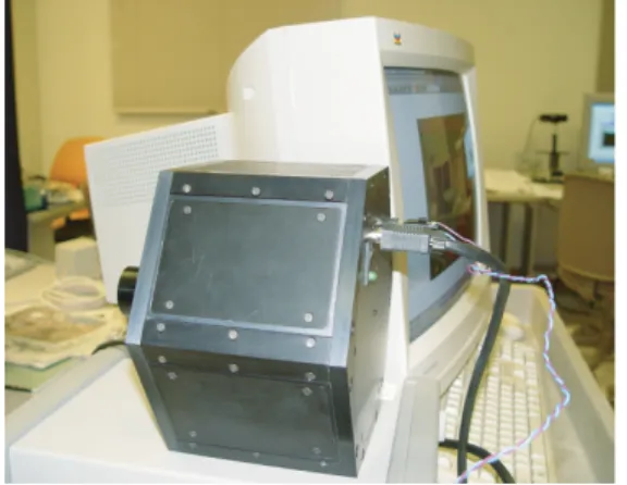
Figure 1. The camera developed to capture HDR video

This results in a large system of linear equations. We use the fast and accurate 3D multigrid algorithm in [18] to it-eratively find the optimal solution to minimize Equation 1. Due to the use of diagonally oriented grids, this algorithm does not need any interpolation when prolongating from a coarse grid onto a finer grid. Actually, a ’red-black’ Jacobi iteration of the residual between the intensity Laplacian and divergence of gradient field avoids interpolation. Most im-portantly, its speed of convergence is much better than usual multigrid scheme.

4

Experimental Results

4.1

HDR Video Capture

We use a split aperture camera [1] developed to capture the HDR video. The camera uses a corner of a cube as a 3-faced pyramid and three CCDsensors. Three thin-film neutral density filters with transmittances of 1, 0.5 and 0.25 are put in front of the sensors respectively. We use Matrox multichannel board capable of synchronizing and capturing three channels simultaneously. The three sensors and the pyramid were carefully calibrated to ensure that all the sen-sors were normal to the optical axes. The setup of our HDR video capture devices is shown in Fig. 1.

4.2

Results

We test our 3D video integration algorithm for video HDR compression on a variety of scenarios. To maintain Neumann boundary conditions, during preprocessing, we pad the video cube with 5 pixels in each direction. The first and last 5 frames, and first and last 5 row/column pix-els of each frame input to the algorithm are all black. The

attenuation parameterβ in Equation 5 is set to 0.15 in all experiments.

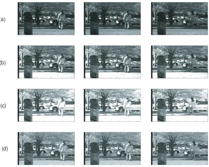
Fig. 2 shows an example of three videos captured using our camera. Due to the shadow of the trees and strong sun-light, none of the individual sensors can capture the whole range of this dynamic scene. For example, the trees and the back of the walking person are too dark in (a) and (b), but too bright in (c). The light bar in (a) is almost totally dark, and the ground is overexposed in (b) and (c). How-ever, the video obtained using our 3D video integration al-gorithm can capture almost everything clearly in the scene. The detailed motion of the tree leaves is also visible.

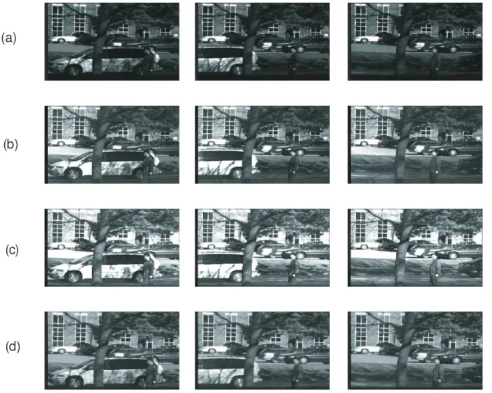
Fig. 3 shows a challenging example with large move-ment in the scene, a walking person with car in motion on the road. The shadow of the tree on the car is clear in (a) but washed out in (b) and (c). The details of the tree are lost in (a) and (b). The background buildings are overexposed in (b) and (c). The cars, shadow, person and background are all captured in our reconstructed video using 3D video integration algorithm, while achieving temporal coherence in luminance. The motion blur of the moving car is main-tained. We believe our results are superior to other HDR hardware or software solutions shown for scenes with large motion.

In our practice, the computational speed of 3D Poisson Solver using diagonal multigrid can speed up the integra-tion step, though it is still computaintegra-tionally intensive. The diagonal multigrid algorithm has improved the speed up to twice as fast as correspondingly simple multigrid algorithm. Currently, our Matlab implementation takes approximately 900 seconds for256×256resolution video with 35 frames. A C/C++ implementation will help to further improve the speed.

5

Conclusions and Future Work

In this paper, we have presented a new approach to cap-ture and display high dynamic range videos. Using a split aperture camera, we capture a high dynamic range real-world scene. Using a gradient-based 3D integration algo-rithm applied to video, we compress the high dynamic range of the video for display on low dynamic range devices.

Achieving the integrability of gradient field is still an open problem. To apply this method to high resolution videos, we need to avoid the minor but perceptible spatial smoothing of intensities. We are investigating the theoret-ical aspects and applications of a set of techniques for im-age reconstruction from mixed gradient fields. In addition, some other methods may also provide temporal consistent video. In the future, we will explore other methods for com-parison with our method. Finally, a modified approach to improve efficiency which is using two-frame constrains in-stead of the whole video is under development.

(a)

(b)

(c)

(d)

Figure 2. Experimental results on high dynamic range video. Rows (a)-(c): The three video sequences obtained by split aperture camera; The brightness of the three videos are in ratios 1:2:4; Row (d): The video obtained using our 3D video integration algorithm. The size of video is256×256×35

References

[1] M. Aggarwal and N. Ahuja. High dynamic range panoramic imaging. Proc. International Conference on Computer Vi-sion (ICCV), pages 2–9, July 2001.

[2] V. Brajovic and T. Kanade. A sorting image sensor: An ex-ample of massively parallel intensity-to-time processing for low latency computational sensors. IEEE conf. on Robotics and Automation, pages 1638–1643, Apr. 1996.

[3] P. Debevec and J. Malik. Recovering high dynamic range ra-diance maps from photographs. SIGGRAPH 97, Aug. 1997. [4] F. Durand and J. Dorsey. Fast bilateral filtering for the dis-play of high-dynamic-range images. ACM Transactions on Graphics (TOG), 21(3):257–266, 2002.

[5] R. Fattal, D. Lischinski, and M. Werman. Gradient domain high dynamic range compression. ACM Transactions on Graphics (TOG), 21(3):249–256, July 2002.

[6] G. Finlayson, S. Hordley, , and M. Drew. Removing shad-ows from images. ECCV, pages 823–836, 2002.

[7] S. Kang, M. Uyttendaele, S. Winder, and R. Szeliski. High dynamic range video. SIGGRAPH’03, 61:1–11, 2003. [8] R. Kimmel, M. Elad, D. Shaked, R. Keshet, and I. Sobel. A

variational framework for retinex. HPL-1999-151R1, 1999. [9] M. Konishi, M. Tsugita, M. Inuiya, and K. Masukane. Video camera, imaging method using video camera, method of operating video camera, image processing apparatus and method, and solid-state electronic imaging device. U.S. Patent5420635, May 1995.

[10] E. Land and J. McCann. Lightness and the retinex theory. J. Opt. Soc. Am., 61:1–11, 1971.

[11] S. Mann, C. Manders, and J. Fung. Painting with looks: Pho-tographic images from video using quantimetric processing. ACM Multimedia, pages 117–126, 2002.

(a)

(b)

(c)

(d)

Figure 3. Experimental results on high dynamic range video. Rows (a)-(c): The three video sequences obtained by split aperture camera; The brightness of the three videos are in ratios 1:2:4; Row (d): The video obtained using our 3D video integration algorithm. The size of video is256×256×35

[12] T. Mitsunaga and S. Nayar. Radiometric self calibration. IEEE Computer Society Conference on Computer Vision and Pattern Recognition (CVPR’99), 1:374–380, 1999. [13] T. Mitsunaga and S. Nayar. High dynamic range imaging:

Spatially varying pixel exposures. IEEE Computer Soci-ety Conference on Computer Vision and Pattern Recognition (CVPR’99), 1:372–479, 2000.

[14] S. K. Nayar and V. Branzoi. Adaptive dynamic range imag-ing: Optical control of pixel exposures over space and time. ICCV, 2003.

[15] P. P`erez, M. Gangnet, and A. Blake. Poisson image editing. Siggraph, pages 313–318, 2003.

[16] R. Raskar, A. Ilie, and J. Yu. Image fusion for context en-hancement and video surrealism. NPAR’04, 2004.

[17] E. Reinhard, M. Stark, P. Shirley, and J. Ferwerda. Photo-graphic tone reproduction for digital images. SIGGRAPH, pages 267–276, 2002.

[18] A. Roberts. Fast and accurate multigrid solution of poissons equation using diagonally oriented grids. Numerical Analy-sis, July 1999.

[19] K. Saito. Electronic image pickup device. Japanese Patent07-254965, Feb. 1995.

[20] D. Socolinsky and L. Wolff. A new visualization paradigm for multispectral imagery and data fusion. CVPR, 1, June 1999.

[21] R. Street. High dynamic range segmented pixel sensor array. U.S. Patent 5638118, June 1997.

[22] J. Tumblin, J. Hodgins, and B. Guenter. LCIS: A bound-ary hierarchy for detail-preserving contrast reduction. Proc. ACM SIGGRAPH, pages 83–99, 1999.

[23] H. Wang, R. Raskar, and N. Ahuja. Seamless video com-positing. IEEE, International Conference on Pattern Recog-nition (ICPR), 2004.