Development and Application of a Satellite-based Convective Cloud Object-Tracking Methodology: A Multipurpose Data Fusion Tool

Development and Application of a Satellite-based Convective Cloud Object-Tracking Methodology: A Multipurpose Data Fusion Tool

Justin M. Sieglaff, Daniel C. Hartung, Wayne F. Feltz, Lee M. Cronce

Cooperative Institute for Meteorological Satellite Studies, University of Wisconsin-Madison, Madison Wisconsin

Valliappa Lakshmanan

Cooperative Institute for Mesoscale Meteorological Studies, University of Oklahoma and NOAA/National Severe Storms Laboratory, Norman Oklahoma

Corresponding author address: Justin Sieglaff, 1225 West Dayton Street, Madison, Wisconsin

53706. E-mail: [email protected] Telephone: 608.265.5357 Fax: 608.262.5974

Submitted to Journal of Applied Meteorology and Climatology on: 07 February 2012

ABSTRACT

Studying deep convective clouds requires the use of available observation platforms with high temporal and spatial resolution, as well as other non-remote sensing meteorological data (i.e. numerical weather prediction model output, conventional observations, etc.). Such data is often at different temporal and spatial resolutions, and consequently there exists the need to fuse these different meteorological datasets into a single framework. This paper introduces a

methodology to identify and track convective cloud-objects from convective cloud infancy (as few as 3 GOES infrared (IR) pixels) into the mature phase (hundreds of GOES IR pixels) using only geostationary imager IR-window observations.

The object tracking system described within builds upon the Warning Decision Support System – Integrated Information (WDSS-II) object tracking capabilities. The system uses an IR-window based field as input to WDSS-II for cloud-object identification and tracking and a UW-CIMSS developed post-processing algorithm to combine WDSS-II cloud-object output. The final output of the system is used to fuse multiple meteorological datasets into a single cloud-object framework. The cloud-object tracking system performance is quantitatively measured for 34 convectively active periods over the central and eastern United States during 2008 and 2009. The analysis shows improved object-tracking performance with both increased temporal resolution of the geostationary data and increased cloud-object size. The system output is demonstrated as an effective means for fusing a variety of meteorological data including: raw satellite observations, satellite algorithm output, radar observations and derived output,

1. Introduction

Deep convective clouds develop on the order of minutes to hours. To observe the growth of deep convection from infancy to maturity, it is necessary to monitor these clouds at high temporal and spatial resolution. Geostationary imagers (e.g. GOES, SEVIRI, JAMI, etc.) are ideal instruments for investigating these clouds as they offer expansive spatial coverage (regional to fulldisk), high temporal resolution (5-15 minutes), and high spatial resolution (1-4 km)

(Menzel and Purdom 1994; Aminou 2002; Puschell et al. 2002). Ground-based weather radar is another essential tool for examining the development of deep convection. In particular, the Next-Generation Weather Radar (NEXRAD) network provides data at 5-minute temporal resolution and very fine spatial resolution with coverage over the majority of the continental United States (CONUS) (NEXRAD 1985; Leone et al. 1989). In addition to remote sensing tools, forecasting and analyzing deep convection requires the integration of other meteorological datasets including, but not limited to: rawinsonde observations, surface observation networks, numerical weather prediction (NWP) model guidance, lightning detection, and aircraft data (e.g. Benjamin et al. 1991; Johns and Doswell 1992; Moller 2001).

With the variety of available datasets at different spatial and temporal resolutions, there exists a need for an automated system that is capable of fusing the array of meteorological data types into a single framework. Working toward this goal, the University of Oklahoma developed the Warning Decision Support System-Integrated Information (WDSS-II; Lakshmanan et al. 2007a), which has been shown to successfully track radar-based objects through space and time using a variety of NEXRAD fields (Lakshmanan et al. 2003). Lakshmanan et al. (2007a) also showed that WDSS-II can be used for fusing a variety of meteorological data. For the purposes

of this study, an ‘object’ simply refers to a collection of adjacent data pixels grouped into a single entity and given a unique identification tag.

Creating and tracking convective objects using NEXRAD data requires a cloud to produce radar-detectable precipitation. However, clouds grow both vertically and horizontally prior to the detection of a corresponding radar echo. Therefore, it is beneficial to begin tracking cloud-objects prior to significant NEXRAD-observed reflectivity since cloud growth rates can be used to nowcast storm development and future intensity ahead of such NEXRAD signatures (Roberts and Rutledge 2003).

Satellite-based object tracking systems have been developed to assist in the forecasting and nowcasting of convection and for fusing convective-related meteorological datasets. In particular, cloud-object tracking systems such as the Rapidly Developing Thunderstorms (RDT, Morel et al. 2002), Maximum Spatial Correlation Tracking Technique (MASCOTTE, Carvalho and Jones 2001), and Forecast and Tracking the Evolution of Cloud Clusters (ForTraCC; Vila et al. 2008) algorithms are designed to identify convective cloud-objects at the onset of maturity and continue tracking throughout the mature stage. These methods primarily focus on

nowcasting the intensification and areal coverage of convection. Zinner et al. (2008) describes a daytime-only convective cloud-object tracking system (Cb-TRAM) designed to diagnose

convective cloud initiation and growth by fusing satellite observations and NWP model information. However, Cb-TRAM is not capable of retaining a history of the properties of multiple meteorological fields through a cloud-object’s lifetime. Unlike the above satellite-based tracking methods, WDSS-II offers the capability to track and retain historical properties for individual cloud-objects at any user-defined stage of the convective lifecycle.

Lakshmanan et al. (2009) demonstrated through proof-of-concept that it is possible to identify objects within WDSS-II using satellite imager infrared (IR)-window brightness

temperatures. This study presents a convective cloud-object identification and tracking system that utilizes a single geostationary satellite IR-window-based field, the 11-µm top of troposphere cloud emissivity (εtot; Pavolonis 2010a). This convective cloud-object tracking system employs the WDSS-II framework and an additional post-processing utility developed at the Cooperative Institute for Meteorological Satellite Studies at the University of Wisconsin (UW-CIMSS).

The satellite-based convective cloud-object identification and tracking system presented herein is unique in many ways. First, the system is designed to monitor the growth stage of convective clouds from infancy (as few as 3 GOES IR pixels) to satellite maturity (hundreds of GOES IR pixels). Second, the tracking system input (εtot) is derived from IR satellite

observations, allowing for operation both day and night. Moreover, εtot does not rely on brightness temperature (BT) thresholds; this permits the full range of the input data to be processed and object identification to remain independent of season and latitude. Finally, the convective cloud-object tracking system is multipurpose in that it can be used to validate convective initiation algorithms with respect to other meteorological data fields from an object-based perspective, to conduct basic research for further understanding the growth stage of deep convection, and to serve as a foundation for a CI nowcasting tool. This paper is organized in the following format: 1) data used, 2) comprehensive description of convective cloud-object tracking system components, 3) analysis and discussion of system performance, 4) example utility of the system, and 5) conclusions and future work.

High temporal resolution geostationary imager data is used as input into the convective cloud-object tracking system. In this paper, GOES-12 and GOES-13 imager data over the central and eastern CONUS and adjacent oceanic regions (bounded by approximately 25N to 52N and 108W to 65W) are used to demonstrate and test the performance of the system for 34

convectively active periods during 2008 and 2009 (periods selected include both daytime and nighttime scenes). The input dataset for the WDSS-II component of the convective cloud-object tracking system is the 11-µm top of troposphere cloud emissivity (εtot; Pavolonis 2010a), which can be described as a background-corrected emissivity (clear-sky absorption and surface emissivity) that a cloud would exhibit if it were located at the tropopause. The unitless values range from 0.0 to 1.0, where 1.0 signifies that the cloud is at the tropopause and a value near 0.0 is indicative of a cloud just above the Earth’s surface. The εtot employs the tropopause height extracted from the Global Forecast System (GFS; Kanamitsu 1989) output, although any NWP model data could be used. Spatially, the εtot maintains the gradients observed in the 11-µm brightness temperature (BT) field; but unlike BT, the εtot field is nearly independent of season and latitude. Therefore, εtot was chosen over the IR BT for cloud-object creation. For example, a mature convective cloud nearing the tropopause will always have εtot values approaching 1.01, whereas the BT of such a cloud can vary on the order of tens of degrees Kelvin both latitudinally and by season. In addition, εtot is only calculated for cloudy pixels [as determined by the

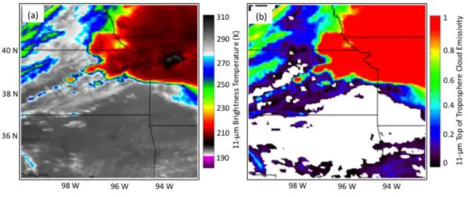
Heidinger (2010) cloud mask] and as a result, clear-sky pixels are excluded from cloud-objects. Figure 1 shows an example of the εtot field compared to the IR-window BT field. It is evident that spatial gradients observed in the BT field are preserved in the εtot field; thunderstorm anvils

have εtot values approaching 1.0, signifying that they are at or near the tropopause, while εtot values are not computed for clear-sky pixels (Fig. 1).

3. Convective Cloud-Object Tracking Methodology

The convective cloud-object tracking system is broken down into two main components: 1) a WDSS-II component that uses εtot for cloud-object generation and initial tracking and 2) a UW-CIMSS developed post-processing system that reduces broken convective cloud-object tracks. A high level flow chart of the processing system is shown in Figure 2 and is referenced throughout Section 3. The output from the convective cloud-object tracking system and

statistical post-processing methodology can be used to fuse any type of meteorological data into the cloud-object framework.

3a. WDSS-II using εtot

The primary WDSS-II algorithm utilized in the convective cloud-object tracking methodology is w2segmotionll (simply referred to as WDSS-II throughout the text). WDSS-II not only builds cloud-objects at any number of user-specified size scales using the enhanced watershed transform method (Lakshmanan et al. 2009), but also provides a variety of options for tracking cloud-objects through space and time. The WDSS-II cloud-object creation and tracking process is discussed in moderate detail throughout the remainder of this section; for complete details on the WDSS-II object identification algorithm, the reader is referred to Lakshmanan et al. (2003) and Lakshmanan et al. (2009).

In our configuration, the εtot field is processed by WDSS-II on three spatial scales (Fig. 2, Section a). Each scale refers to the minimum number of pixels that a cloud-object must achieve before the growth is terminated by WDSS-II on that particular scale. Additionally, if a cloud-object does not achieve the minimum number of pixels required for a given scale, it is pruned by the enhanced watershed technique (Lakshmanan et al. 2009). WDSS-II builds cloud-objects on each scale by first determining all local maxima in the εtot input field. Each cloud-object is then filled down from the local maxima to smaller values of εtot based upon the user-configured data depth and scale size thresholds. It should be noted that the configuration discussed here was chosen heuristically after testing multiple configurations; the results of each individual test configuration are not shown. Although the system is referred to as a convective cloud-object tracking system, all clouds (εtot values) are input into WDSS-II for object creation and tracking. The WDSS-II configuration described below is specifically tailored for tracking convective clouds from infancy to maturity; we are not concerned with the object tracking performance for synoptic cloud systems, clouds associated with jet streaks, or large cirrus shields.

Cloud-objects are grown within WDSS-II from the local maxima in the εtot field by first grouping continuous pixels with εtot values greater than 0.5 into unique clusters. Values between 0.5 and 1.0 are grouped together in order to maximize computational efficiency and to delineate middle- to upper-tropospheric cloud features as single entities. Specifically, this configuration does not seek to capture small areas within a developing thunderstorm anvil, but rather is designed to encompass the entire developing thunderstorm tower and anvil in one cloud-object. The cloud-object building continues on each scale in 0.025 increments for εtot values between 0.50 and 0.10. Each cloud-object on a given scale grows until the minimum size threshold for

minimum size for particular scales are pruned. The small bin-size (0.025) for lower- to middle- tropospheric clouds is chosen to keep cloud-objects from spatially growing too large (i.e. merging features into large objects that a human analyst would consider separate entities).

Cloud-objects are grown on three scales: 3, 15, and 30 pixels [the pixels are a 0.04-degree grid, which is approximately the resolution of the input GOES Imager IR data (Menzel and Purdom 1994)]. After testing a range of sizes (not shown), the above combination yielded the best performance. The smallest scale (3 pixels) is necessary to capture convective clouds in the very early stages of growth. The two larger scales (15 and 30 pixels) allow cloud-objects to grow large enough to encompass the vast majority of the convective cloud. These multiple scales are designed to resolve convective clouds at different stages of growth from infancy to maturity. A single WDSS-II output scale by itself is not sufficient for capturing all phases of convective cloud growth, and it is therefore necessary to combine all three WDSS-II output scales into a merged file through a post-processing step.

Within WDSS-II, cloud-objects are assigned unique object ID numbers and tracked across space and time. WDSS-II offers several options for tracking cloud-objects. Many of the WDSS-II object tracking options do not rely on object overlap between two times, but rather minimize a cost function (TITAN, Dixon and Wiener 1993; Lakshmanan and Smith 2010) for a given object at one time versus candidate objects at the following scan time. The reader is referred to Lakshmanan and Smith (2010) for a complete description of WDSS-II object tracking methods.

The WDSS-II OLDEST object tracking option was determined most skillful for our application, with preference for maintaining the oldest cloud-object when multiple candidates

investigate relationships between real-time, historical and forecast data sets for individual

evolving cloud-objects, methods such as Multiple Hypothesis Tracking (MHT; Root et al. 2011), which allow for the modification of historical object tracks based on current information, are not applicable to this work. The WDSS-II OLDEST object-tracking methodology uses a user-configurable search radius for each scale. The search radius configuration selected for the convective cloud-object tracking system is equal to the greater of the object radius and 20 km. The radius of a cloud-object is defined as the radius of a circle with the same total area of the cloud-object. WDSS-II uses an object’s centroid location and search radius to look for

companion objects; in other words, an object’s centroid from one time to the next must be within the search radius to be successfully tracked (unique object ID maintained between two times). The dynamic and 20 km maximum search radii thresholds allow small objects to be successfully maintained between GOES imager scans. Additionally, the WDSS-II user configuration

specifies to only consider adjacent times when tracking objects [e.g. an object ID is not allowed to coast (disappear and then later reappear at a later time)].

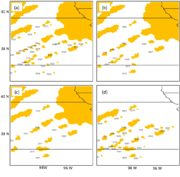
The two-dimensional fields for each of the three cloud-object scales (and their associated object ID numbers) are then combined in a post-processing step to create one unique set of merged objects. An example of the three individual WDSS-II cloud-object scales and the final post-processed merged objects valid at the same time as Figure 1 (2002 UTC 15 May 2009) are shown in Figure 3. Figure 3a clearly illustrates the ability of small convective objects to be identified on scale 1. Some of the small objects on scale 1 are part of larger objects on scales 2 and 3 (Figs. 3b,c), while other objects are unique to scale 1. The UW-CIMSS post-processing component of the system that combines the three WDSS-II scales (Fig. 3d) is fully described in

3b. Cloud-object Post-Processing System 3.b.1 – Main Cloud-Object Post-Processing

After WDSS-II cloud-object creation and tracking are complete, a post-processing routine combines the three cloud-object scales into a set of final merged objects at each time. These cloud-objects are used for fusing meteorological data (Fig. 2, Section b) into a single framework. This post-processing step is an essential part of the system as it ensures that cloud-objects encompass the fullest possible extent of a convective cloud while not allowing cloud-objects to grow spatially unbounded, similar to how a human would identify convective cloud-objects. In addition to merging the three WDSS-II scales into a set of final cloud-objects, a series of tests are conducted to assign and maintain temporally consistent object IDs between consecutive satellite scans. This step is critical when the WDSS-II object tracking fails and a cloud-object

undesirably changes ID between two satellite scans. The main cloud-object post-processing procedure and two user options are described in detail below and illustrated in Tables 1-3.

The post-processing algorithm loops through the cloud-objects on scale 1 (smallest scale) in descending order of maximum cloud-object εtot. Each cloud-object on scale 1 is potentially grown larger by combining overlapping objects on the larger scales 2 and 3. The newly grown cloud-object is stored as a temporary merged cloud-object (Table 1: Steps 1-3d) and is assigned the scale 1 object ID so long as the particular ID is not already in use. It is necessary to use the object ID from the smallest scale since small objects (less than 15 pixels) will only be identified on scale 1. As a consequence of how the merged object field is populated (i.e. descending order

is imperative that two objects never be assigned the same final merged object ID, if the scale 1 object ID is already in use within the field of temporary merged cloud-objects, the temporary merged object is assigned an object ID of -333. The procedure for reassigning object IDs to temporary merged objects previously assigned a placeholder ID of -333, will be discussed later.

Table 1, step 3e, and associated subtests, are used to assign the temporary merged cloud-object a final merged cloud-object ID. Recall that temporary merged cloud-cloud-objects are initially assigned their corresponding scale 1 object ID. Scale 1 objects often have limited spatial extent (sometimes just a subset of a cloud) because the WDSS-II object-building enhanced watershed technique stops as soon as an included bin of data results in an object size of at least 3 pixels. These small, scale 1 objects include both full cloud-objects that are in their infancy as well as the ‘cores’ of more developed cloud-objects. Since the scale 1 objects only capture the ‘core’ of more developed convection, scales 2 and 3 are used to fill out the merged cloud-object to encompass more of the storm.

One limitation of the WDSS-II object tracking system is that it has the highest failure rate for scale 1 objects due to their small spatial extent, rapid storm evolution during the growth stage, and a potentially large distance traveled during GOES scan gaps relative to their size (i.e. especially 3-hourly, 30-minute temporal data gaps). In this context, failure refers to when a scale 1 object incorrectly changes ID between the previous (tprev) and current (tcurr) satellite scan-times. Further analysis of this assertion is explored in Section 3c. To overcome these challenges, a series of tests were devised within the UW-CIMSS post-processing algorithm that utilizes the final merged cloud-object field at tprev and the WDSS-II cloud-objects on scales 2 and 3 at tprev and tcurr to assign final merged object IDs at tcurr.

Step 3e (Table 1) initially identifies all final merged cloud-objects at tprev that spatially overlap with the temporary merged cloud-object, similar to the overlap association technique used by Morel et al. 1997. It is assumed that any object at tprev that overlaps with the temporary merged cloud-object at tcurrmay be the same object; these objects are termed ‘candidate objects’. The WDSS-II object tracking (and associated object ID assignment) in our application improves for scales 2 and 3 relative to scale 1 (further discussed in Section 3c). This improvement stems from cloud-objects on scales 2 and 3 being larger, and consequently less sensitive to the distance traveled between GOES scans relative to the object tracking search radius. Each candidate object is tested for WDSS-II scale 2 or scale 3 ‘consistency’ between tprev and tcurr. Any object that has the same scale 2 or scale 3 object ID at tprev and tcurr exhibits ‘consistency’ and is retained, while all others are no longer considered. The areal overlap between the temporary merged object and the remaining candidate objects is computed. Finally, the temporary merged cloud-object is assigned the ID of the candidate object that has the most areal overlap and whose ID is not already in use within the temporary merged cloud-object field. If no candidate objects qualify, the object is purged.

If the WDSS-II scales and final merged cloud-object fields do not exist at tprev, (e.g. the first time-step when running the convective cloud-object system), step 3e in Table 1 is skipped and processing continues at step 3f. Table 1, step 3f simply purges objects that were not assigned an object ID other than -333 by the aforementioned tests (e.g. their temporary merged object did not overlap with any unused final merged cloud-objects at tprev).

Since the primary motivation for developing this convective cloud-object tracking system was to fuse a variety of meteorological datasets for studying the growth and maturation of deep convection, it is desirable to track final merged objects into the mature phase of the thunderstorm lifecycle. One research project at UW-CIMSS utilizes this system to validate the University of Wisconsin Convective Initiation/Cloud-Top Cooling (UWCI/CTC) algorithm (Sieglaff et al. 2011) against a variety of NEXRAD fields. Initial results of this project have suggested that even though a number of final merged cloud-objects achieved a moderate to strong radar

reflectivity (45- to 55-dBZ), many failed to strengthen to intense reflectivity values (60+ -dBZ). It is understood that each convective cloud-object that develops a 45-dBZ radar echo will not necessarily intensify to 60-dBZ; however, the drop off in sample size between the two

reflectivity classifications was larger than expected given the convectively active periods that were being evaluated. Further investigation revealed that many convective cloud-objects were merged into conjoined larger objects due to spatially connected thunderstorm anvils. These much larger cloud-objects were then purged since their size exceeded the maximum 1000-pixel size threshold described in Section 3.b.1. The top-down satellite observations, in combination with horizontal anvil expansion, prevented the objects from being treated as individual entities for a sufficient amount of time. In order to address this problem from a validation perspective, an option was added to the UW-CIMSS post-processing methodology that tracks the core of mature thunderstorms for one to four additional GOES imager scans than was otherwise possible with the system. It is important to note that tracking the core of mature thunderstorms is

sufficient for a validation type study in which collocating satellite algorithm and radar signals within a cloud-object is necessary to compute Probability of Detection (POD) and Probability of

False Detection (POFD) statistics, but is undesirable for other tasks such as objectively quantifying the areal size or rate of areal expansion of a cloud-object with time.

The mature object extension is included in the final merged cloud-object field upon completion of Section 3.b.1. The implementation of the mature object extension uses a secondary WDSS-II cloud-object tracking run and similar overlap concepts as discussed in Section 3.b.1 (Fig. 2, Section b). The mature object extension methodology is detailed below and illustrated in Table 2.

A secondary WDSS-II run, similar to the primary WDSS-II run, is performed for the mature object extension. Three larger WDSS-II object scales (e.g. 20, 40, and 60 pixels for scales 1, 2, and 3, respectively) are used for the mature configuration. In addition, the mature extension only uses εtot values from 0.9 to 1.0 with a binsize of 0.025. Similar to the initial WDSS-II object-tracking run, the mature run utilizes the OLDEST object ID tracking method with an object search radius of the maximum of the object radius and 50 km.

The three mature WDSS-II size scales are combined in a similar manner as to that described in Section 3.b.1. (Table 2, steps 1-3d). After the merged mature objects are created, each object is looped through (Table 2, step 3e). Merged mature cloud-objects that do not overlap with final merged cloud-objects at tcurr, but overlap with final merged cloud-objects at tprev, are considered candidate objects. This routine identifies situations where 1) a mature merged object exists based upon the secondary WDSS-II configuration at tcurr, and 2) the mature merged object overlaps with a final merged object at tprev, but 3) does not overlap with a final merged object at tcurr. This suggests that without the mature extension applied, the final merged cloud-object disappeared between tprev and tcurr.

In these situations, the disappearance of a final merged cloud-object is often due to the merging of convective anvils into a larger object that exceeds the maximum size threshold. When this is the case, a new cloud-object, identical to the mature merged cloud-object, is temporarily inserted into the final merged object field at tcurr (Table 2, step 3e). The new object is assigned the final merged object ID from tprev that had the maximum overlap with the mature merged object and does not already exist in the final merged cloud-object field at tcurr. Should no object meet the above criteria, the temporary object in the final merged cloud-object field is purged.

Figure 4 demonstrates how the mature object extension can preserve a cloud-object longer in time than otherwise possible with the convective cloud-object tracking system. Note that in Figure 4b, the developing convection in central Kansas is no longer a valid object. Figure 4d demonstrates how incorporating the merged objects from the mature extension (Fig. 4c) into the final merged objects from the main cloud-object procedure (Fig. 4b) allows for the cores of objects 6056 and 5312 to be restored to the final merged object field (compare Figs. 4b and 4d).

3.b.3 –User Option: Merged-Object Absorption

When using the convective cloud-object tracking system as a validation tool, it is essential to identify when two cloud-objects at tprev merge into one cloud-object at tcurr. The following scenario further illustrates this point: Two adjacent developing thunderstorms are each characterized by a unique final merged object ID at tprev, a satellite indication of convective cloud growth (i.e. a cooling cloud-top signal), and have an observed radar reflectivity of 35-dBZ. At tcurr, the two cloud-objects merge into a single cloud-object (maintaining one of the two object

eventually develops a 60-dBZ reflectivity on radar. In a validation framework, the object ID that was tracked until it developed a 60-dBZ reflectivity echo would count as a ‘hit’ for that particular reflectivity threshold. However, the object that disappeared as a result of merging would count as a miss for all reflectivity thresholds in excess of 35-dBZ when in actuality, it may have strengthened on radar after the two satellite objects at tprev merged. Therefore it is important to define an attribute for each final merged cloud-object that identifies if and when it merges with another object in order for validation statistics to dismiss such objects upon absorption. To address this need, the UW-CIMSS post-processing system has incorporated a merged-object absorption option that identifies the time that an object is absorbed by another object at tcurr. The full methodology of this option is described in detail below and illustrated in Table 3.

After the tcurr final merged object field has been created as described by Section 3.b.1 (and optionally 3.b.2) and when final merged objects at tprev are available (e.g. not the first time in a processing sequence), each final merged object at tprev is checked for existence within the tcurr final merged object field. The objects at tprev that do not exist at tcurr are looped over as shown in Table 3. The steps in Table 3 help identify when an object at tcurr absorbs an object that existed at tprev. If the object at tprev overlaps with an object at tcurr, yet does not exist at tcurr, it is assigned an absorbed time of tcurr. Table 3, step 1.b.ii accounts for objects that existed at tprev but do not exist at tcurr and do not reside within an object at tcurr. In these cases, the εtot field is sampled at the tprev footprint; if the maximum εtot at tcurr within the tprev footprint is greater than or equal to 0.50, the object is considered to have been absorbed into an object at tcurr that exceeded the

maximum object size threshold and hence was purged2. Finally, the object from tprev is assigned an absorbed time of tcurr.

3c. Discussion of Convective Cloud-object Tracking Performance

One metric for determining the performance of the cloud-object tracking system is the amount of time (in minutes) that cloud-objects are successfully tracked as a function of the maximum εtot achieved during the object’s lifetime (Fig. 5). Figure 5 and Table 4 show that as cloud-objects grow higher into the troposphere (and consequently exhibit larger εtot values), the mean lifetime increases from ~35 minutes for cloud-objects remaining in the lower troposphere (maximum εtot between 0.20 and 0.30) to near 155 minutes for cloud-objects approaching the tropopause (maximum εtot greater than 0.90). The progression to longer lifetimes for objects with increased vertical development is consistent with the concept that a cumulonimbus is more organized and hence longer-lived than a towering cumulus, and likewise a towering cumulus is more organized and often longer-lived than a shallow cumulus cloud (Wallace and Hobbs 1977). The distributions of object lifetime are much wider for convective cloud-objects near the

tropopause (thunderstorms) than lower tropospheric cloud-objects (shallow cumulus fields) (Fig. 5). In fact, the cloud-object lifetime distribution for thunderstorms (cloud-objects with

maximum εtot greater than 0.90) weakly peaks near 80 minutes with a substantial tail extending to 300+ minutes. An analysis of thunderstorm cloud-objects (not shown) suggests that the weak peak near 80 minutes can be attributed to storms that develop in linear regimes and merge into large anvil objects that eventually become pruned; the linear convection from 15 May 2009 in

Figure 4a is one such example. Thunderstorm cloud-objects lasting for 120+ minutes consist largely of isolated storms, often dryline scenarios or initial cells in linear regimes. These distributions lend confidence that the convective cloud-object tracking system is performing as expected.

A strength of the cloud-object tracking system is that it can be used with data from any geostationary satellite platform (with sufficient temporal resolution). The εtot field is computed using 11-µm IR observations measured by all operational geostationary imagers (GOES, Menzel and Purdom 1994; SEVIRI, Aminou 2002; JAMI, Puschell et al. 2002, etc.) and the Heidinger (2010) cloud mask is adaptive to the different available spectral channels on various satellite imagers.

In general, as the temporal resolution of the satellite increases, the cloud-object tracking becomes more accurate. Current GOES imagers have a routine temporal resolution of ~15 minutes over CONUS (alternating 13- and 17-minute scans); though in cases of expected severe convection, rapid scan mode is invoked, providing up to 5-minute temporal resolution over CONUS (Hillger and Schmit 2007). Independent of the GOES scan mode, 30-minute gaps occur every 3 hours (beginning at 00 UTC) due to scheduled fulldisk scans. The 30-minute gaps can be a significant source of error in the cloud-object tracking system, especially for spatially small objects and objects that grow tremendously within those 30-minute periods. Convective cloud-objects that have already developed an anvil are typically tracked successfully through these 30-minute temporal gaps.

Figure 6a demonstrates how the temporal resolution of a GOES scan pattern impacts the convective cloud-object tracking system performance. For periods in which GOES is in rapid

cloud-objects retained following a rapid scan gap (Fig. 6a). As the temporal resolution of the satellite coarsens, the object tracking performance degrades with the cloud-object retention rate decreasing to 59% for the GOES routine scan mode (13- to 17-minute scan gaps) and 40% for larger 20+ minute GOES scan gaps (Fig. 6a). The absolute retention rates are not necessarily important since the baseline rate is not quantified; however, the overall increase in retention rate with increased satellite temporal resolution is noteworthy3. The future GOES Advanced

Baseline Imager (ABI) onboard GOES-R will provide 5-minute temporal coverage over CONUS and at least 15-minute coverage over the fulldisk (possible 5-minute fulldisk depending on which scanning pattern is chosen) (Schmit et al. 2005). Based on the above analysis, the increased temporal sampling of GOES-R ABI will greatly reduce the errors associated with the cloud-object tracking system. Though not extensively tested nor shown in the text, this cloud-cloud-object tracking system has been initially tested with SEVIRI data (15-minute fulldisk coverage) with encouraging results. Porting to other operational geostationary imagers is also possible, although this has not been exercised. However, it is recommended that the imager have predominately 15-minute or better temporal resolution to successfully use the tracking system.

As referenced in Section 3.b.1, the spatial size of cloud-objects also impacts the system performance. Previously it was stated that a limitation of the WDSS-II object tracking system is that it has the highest failure rate for scale 1 objects due to their small spatial extent, rapid storm evolution in the growing stage of convection, and potentially large distance traveled during GOES scan gaps. Figure 6b shows the convective cloud-object retention rate as a function of cloud-object size in number of pixels. The smallest objects (less than 15 GOES IR pixels) that

only exist on scale 1 exhibit the lowest retention rate (49%), and the retention rate increases as the cloud-object size increases (Fig. 6b). For cloud-objects with at least 15 pixels but less than 30 pixels (objects that exist on scale 1 and scale 2), the retention rate increases to 64%. A

similar upward trend is observed for cloud-objects with at least 30 pixels and less than 100 pixels (objects existing on scales 1, 2, and 3) with a retention rate of 74% and for cloud-objects of 100+ pixels exhibiting a retention rate of 81%.

In summary, as the temporal resolution of the geostationary imager increases, the object tracking system performance improves. Twenty minute and larger scan gaps with GOES data can significantly decrease system performance. In addition, object tracking performance increases as object size increases and object tracking lifetime increases as cloud-objects reach higher into the troposphere. These two points give confidence that the objects of greatest interest (i.e. those that begin to develop into and have developed into thunderstorms) have the highest likelihood of successful tracking.

3d. Example of Fusing Convective Cloud-object Tracking Output and Meteorological Fields After the cloud-object post-processing routine is complete, the final merged cloud-objects can be used as a vehicle to fuse any meteorological datasets for a wide array of potential utilities. UW-CIMSS has developed an additional statistical post-processing system that uses the

convective cloud-objects to fuse raw satellite observations, satellite algorithm output [e.g. UWCI/CTC Cloud-Top Cooling Rate (Sieglaff et al. 2011), GOES cloud phase (Pavolonis and Heidinger 2004; Pavolonis et al. 2005; Pavolonis 2010b), GOES cloud height (Heidinger 2011), GOES visible optical depth and effective radius (Walther et al. 2012), etc.], NEXRAD

reflectivity, Vertically Integrated Liquid (VIL), Maximum Expected Size of Hail (MESH), etc.], NWP model fields and derived parameters, National Lightning Detection Network (NLDN) data (Cummings et al. 1998), and Storm Prediction Center (SPC) storm reports. The focus of this paper is not to technically detail the statistical post-processing system, but rather to demonstrate the utility and ease of fusing meteorological data using the convective cloud-object tracking system output.

On a high level, the statistical post-processing system is simply a data structure with a unique entry for each cloud-object ID. For each cloud-object (data structure entry), any number of statistics for any number of meteorological (or non-meteorological) data fields and object-related metadata can be stored. For example, each data structure entry might include the first time and last time that an object exists, as well as histograms of different satellite, radar, and NWP fields for each time the object was present or at the temporal resolution of the respective meteorological field. From these histograms it is possible to compute and extract information such as the first time that specific radar thresholds are attained for a given cloud-object, the time rate of change of different satellite observations and derived products, and when the first NLDN strike was detected within a cloud-object.

Figure 7a shows the final merged cloud-object output from the convective cloud-object tracking system for 2215 UTC 13 May 2009 over the Central Plains of the US. The large object over eastern Kansas is a mature, supercell thunderstorm with a line of developing convective clouds extending to the southwest into south-central Kansas and northwestern Oklahoma. Northeast of the cell over northwestern Missouri, the cloud-objects have been purged because they have grown in excess of the user-defined 1000-pixel maximum size threshold described in

Section 3.b.1. The εtot panel in Figure 7b is shown as a reference from which the cloud-objects were built.

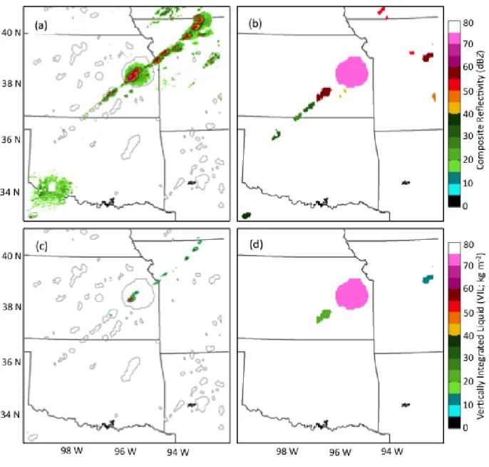
Figure 8 illustrates how NEXRAD fields are fused into the cloud-objects by the statistical post-processing system. Quality-controlled NEXRAD data from the National Severe Storms Laboratory (NSSL; Lakshmanan et al. 2007b) is remapped from its native 0.01-degree horizontal resolution to a 0.04-degree latitude/longitude grid to match the satellite grid, while retaining the 9x9 neighborhood maximum of the original data at each coarsened point. Figures 8a,c show cloud-objects from Figure 7a outlined in gray with composite radar reflectivity and VIL valid at 2216 UTC 13 May 2009 shaded, respectively. Figures 8b,d demonstrate data fusion of cloud-objects filled by the maximum of the composite reflectivity and VIL fields, respectively. The supercell thunderstorm over eastern Kansas has a maximum composite reflectivity in excess of 70-dBZ (maximum VIL in excess of 70 kg m-2), while the developing convective clouds to the southwest have maximum composite reflectivity values ranging from 20 to 55-dBZ (maximum VIL ranges from 0 to 15 kg m-2). The intense composite reflectivity to the northeast of the supercell thunderstorm in eastern Kansas is not shaded on the cloud-object plots because those objects exceeded the maximum size threshold and were pruned.

Figure 9 demonstrates how additional meteorological data is fused into the cloud-object output. Figures 9a,c have cloud-objects from Figure 7a outlined in gray with NLDN lightning strikes colored by age prior to 2215 UTC 13 May 2009 and Rapid Update Cycle (RUC;

Benjamin et al. 1994) Most Unstable CAPE (MUCAPE) shaded and valid at 2200 UTC 13 May 2009, respectively. Figures 9b,d demonstrate data fusion of cloud-objects filled by the elapsed time since the first NLDN strike and by maximum RUC MUCAPE, respectively. The supercell

2215 UTC, while the developing convection to the southwest has yet to produce an NLDN-detected lightning strike. The supercell thunderstorm over eastern Kansas and developing line to the southwest exist in a ribbon of locally high RUC MUCAPE (generally 3500+ J kg-1 K-1), while cloud-objects to the north and west behind the surface cold front (not shown) over central and northern Kansas have much smaller values of MUCAPE.

Two projects at UW-CIMSS currently utilize the convective cloud-object tracking and statistical post-processing systems. The first, described in Section 3.b.2, uses the cloud-object tracking system to determine relationships between UWCI/CTC Cloud-Top Cooling rates and a variety of NEXRAD fields and first NLDN strikes. The goal of that project is to determine the POD and POFD of the UWCI Cloud-Top Cooling rates as a function of different NEXRAD fields. In addition, a lead-time analysis of cloud-top cooling rates as a function of the same NEXRAD fields is being generated. The second project leverages the two systems to compute the time rate of change of an array of satellite cloud-retrieved fields (e.g. εtot, cloud phase, visible optical depth), combined with NWP data and NEXRAD data to probabilistically nowcast the likelihood that a developing convective cloud will produce surface severe weather reports in the subsequent 0-2 hour timeframe. The lead-time of such probabilistic nowcasts ahead of severe weather warnings and radar indicated severe signatures is also being computed.

4. Conclusions and Future Work

Deep convective clouds develop on small spatial and temporal scales (minutes to hours). In order to monitor the growth of convective clouds from infancy into the mature phase, it is necessary to observe these clouds with sufficiently high spatial and temporal resolution.

of high quality data. When using these observational datasets, human analysts do not view individual pixels, but rather individual convective towers or storms (groups of pixels). With the goal of mimicking a human’s subjective interpretation of cloud-objects in an objective automated manner, UW-CIMSS has developed a convective cloud-object tracking system that utilizes the WDSS-II framework developed at the University of Oklahoma to group adjacent cloudy satellite pixels into cloud-objects, similar to how a human would analyze satellite or radar data, and track these cloud-objects through space and time. A UW-CIMSS post-processing utility then merges the WDSS-II output and performs steps to minimize the broken tracks of convective cloud-objects. The convective cloud-object tracking system presented herein is designed to track convective clouds from infancy into the mature phase and provide a means to generate statistics of any number of meteorological fields for each cloud-object within a time period of interest.

The convective cloud-object tracking system uses the 11-µm top of troposphere cloud emissivity (εtot) as input into WDSS-II for cloud-object identification and tracking. The input εtot field is derived using only 11-µm IR radiances (or equivalent), and thus the system is capable of operating both day and night for any geostationary imager with sufficient temporal resolution. The UW-CIMSS developed post-processing system combines three different size scale outputs from WDSS-II into a final set of cloud-objects, minimizing broken cloud tracks in the process.

The performance of the convective cloud-object tracking system was quantitatively discussed. The key findings consist of the following: 1) the finer the satellite temporal

resolution, the better the cloud-object tracking system performs, 2) the larger an object grows, the better the cloud-object tracking system performs (key for tracking cumulus with vertical growth and newly developed cumulonimbus), and 3) cloud-objects that grow higher in the

troposphere (i.e. shallow cumulus). While not discussed within the text, it should be noted that the typical linux research system run-time on a domain covering the central and eastern CONUS and adjacent oceanic regions is approximately 6 minutes per satellite scan, which suggests that this system has the potential to be used in real-time applications.

Since cloud-objects are output on a 0.04-degree grid, it is straightforward to fuse a variety of meteorological data fields into one framework by projecting the data onto the same grid. With the use of a statistical post-processing system, the cloud-object output can be used to fuse raw satellite observations, satellite derived/retrieved fields, NEXRAD observations and algorithm output, NWP fields, NLDN data, and SPC storm reports. In fact, any geo-referenced dataset, including non-meteorological data, can be fused with the cloud-objects through the statistical post-processing system. Two research projects at UW-CIMSS are utilizing the convective cloud-object tracking system and future publications from those projects will further demonstrate the utility of the system.

While the convective cloud-object tracking system was shown to perform well with the current configuration, future work will focus on ways to improve the system. Specifically, focus will be on situations in which a human would analyze two separate convective cloud-objects based on satellite observations, but the two clouds are undesirably merged into a single object using the current configuration (i.e. largely thunderstorm anvils that are connected, but still obviously separate objects to a human analyst). The authors understand that given the top-down perspective from the satellite and nature of thunderstorm anvil expansion, objects will always merge into larger scale convective systems that are pruned by the convective cloud-object tracking system. However, it is desirable to keep two objects separate for an additional few

satellite scans. In essence, one additional routine GOES scan can allow for up to an additional three NEXRAD scans to be incorporated into a cloud-object’s history.

5. Acknowledgements

We would like to extend our appreciation for having the opportunity to perform this work under the NOAA GOES Product Assurance Plan (GIMPAP) program, federal grant number NA10NES4400013. We would also like to acknowledge John Cintineo for his insight and careful review of the manuscript.

References

Aminou, D. M. A., 2002: MSG’s SEVIRI Instrument. ESA Bull., 111, 15-17.

Benjamin, S. G., K. J. Brundage, and L. L. Morone, 1994: The Rapid Update Cycle. Part I: Analysis/model description. NOAA/NWS Tech. Procedures Bulletin 416, 16 pp.

Benjamin, S. G., K. A. Brewster, R. L. Brummer, B. F. Jewett, T. W. Schlatter, T. L. Smith, and P. A. Stamus, 1991: An isentropic three-hourly data assimilation system using ACARS aircraft observations. Mon. Wea. Rev.,119, 888-906.

Carvalho, L.M.V., and C. Jones, 2001: A Satellite Method to Identify Structural Properties of Mesoscale Convective Systems Based on the Maximum Spatial Correlation Tracking Technique (MASCOTTE). J. Appl. Meteor., 40, 1683–1701.

Cummings, K. L., M. J. Murphy, E. A. Bardo, W. L. Hiscox, R. B. Pyle, and A. E. Pifer, 1998: A combined TOA/MDF technology upgrade of the U.S. National Lightning Detection Network. J. Geophys. Res., 103, 9035-9044.

Dixon M., and G. Wiener, 1993: TITAN: Thunderstorm identification, tracking, analysis and nowcasting—A radar-based methodology. J. Atmos. Oceanic Technol.,10, 785-797. Heidinger, A.K., 2011: ABI Cloud Height Algorithm Theoretical Basis Document. NOAA

NESDIS Center for Satellite Applications and Research (STAR), 77 pp.

---, 2010: ABI Cloud Mask Algorithm Theoretical Basis Document. NOAA NESDIS Center for Satellite Applications and Research (STAR), 67 pp.

Hillger, D. W., and T. J. Schmit, 2007: The GOES-13 Science Test: Imager and Sounder Radiance and Product Validations. NOAA Tech. Report NESDIS 125, 88 pp.

Kanamitsu, M., 1989: Description of the NMC Global Data Assimilation and Forecast System. Wea. Forecasting,4, 335-342.

Lakshmanan V., and T. Smith, 2010: An Objective Method of Evaluating and Devising Storm-Tracking Algorithms. Wea. Forecasting, 25, 701-709.

---, K. Hondl, and R. Rabin, 2009: An Efficient General-Purpose Technique for Identifying Storm Cells in Geospatial Images. J. Atmos. Oceanic Technol., 26, 523-537.

---, R. Rabin, and V. DeBrunner, 2003: Multiscale storm identification and forecast. J. Atmos. Res., 67-68, 367-380.

---, T. Smith, G. J. Stumpf, and K. Hondl, 2007a: The Warning Decision Support System – Integrated Information. Wea. Forecasting, 22, 596-612.

---, A. Fritz, T. Smith, K. Hondl, and G. J. Stumpf, 2007b: An automated technique to quality control radar reflectivity data. J. Appl. Meteor. Climatol., 46, 288-305.

---, T. Smith, K. Hondl, G. J. Stumpf, and A. Witt, 2006: A realtime, three dimensional, rapidly updating, heteorogenous radar merger technique for reflectivity, velocity, and derived products. Wea. Forecasting, 21, 802-823.

Leone, D. A., R. M. Endlich, J. Petriceks, R. T. H. Collins, and J. R. Porter, 1989:

Meteorological considerations used in planning the NEXRAD network. Bull. Amer. Meteor. Soc.,70, 4-13.

Menzel, P., and J. Purdom, 1994: The first of a new generation of geostationary operational environmental satellites. Bull. Amer. Meteor. Soc.,75, 757-782.

Moller, A. R., 2001: Severe local storms forecasting. Severe Convective Storms, Meteor. Monogr., 50, American Meteorological Society, 433-480.

Morel, C., S. Senesi, and F. Autones, 2002: Building upon SAF-NWC products: Use of the Rapid Developing Thunderstorms (RDT) product in Meteo-France nowcasting tools.

Proc. 2002 Meteorological Satellite Data Users’ Conf., Dublin, Ireland, EUMETSAT

and Met Eirean, 248-255.

Morel, C., F. Orain, and S. Senesi, 1997: Automated detection and characterization of MCS using the Meteosat infrared channel. Proc. Meteor. Satellite Data Users Conf., Brussels, Belgium, EUMETSAT, 213-220.

NEXRAD, 1985: Next generation weather radar (NEXRAD) algorithm report. NEXRAD Joint System Program Office, Washington, DC.

Pavolonis, M. J, 2010a: Advances in extracting cloud composition from spaceborne radiances: A robust alternative to brightness temperatures, Part I: Theory. J. Appl. Meteor.

Climatol., 49, 1992-2012.

---, 2010b: ABI Cloud Type/Phase Algorithm Theoretical Basis Document. NOAA NESDIS Center for Satellite Applications and Research (STAR), 60 pp.

---, and A. K. Heidinger, 2004: Daytime cloud overlap detection from AVHRR and VIIRS. J. Appl. Meteor., 43, 762-778.

---, A. K. Heidinger, and T. Uttal, 2005: Daytime global cloud typing from AVHRR and VIIRS: Algorithm description, validation, and comparisons. J. Atmos. Oceanic Technol.,

44, 804-826.

Puschell, J. J., H. A. Lowe, J. W. Jeter, S. M. Kus, W. T. Hurt, D. Gilman, D. L. Rodgers, R. L. Hoelter, and R. Ravella, 2002: Japanese Advanced Meteorological Imager: A next generation GEO imager for MTSAT-1R. SPIE Proceedings, 4814, 152-161.

Roberts, R. D., and S. Rutledge, 2003: Nowcasting storm initiation and growth using GOES-8 and WSR-88D data. Wea. Forecasting, 18, 562–584.

Root, B., M. Yeary, and T. -Y. Yu, 2011: Novel storm cell tracking with Multiple Hypothesis Tracking, Preprints, 27th Conf. on Interactive Information Processing Systems (IIPS) (2011), 8B.3, Seattle, WA, Amer. Meteor. Soc. [Available online at

http://ams.confex.com/ams/91Annual/webprogram/Manuscript/Paper184250/AMSAnnua l2011_MHTAbstract.pdf.]

Schmit, T. J., M. M. Gunshor, W. P. Menzel, J. Li, S. Bachmeier, and J. J. Gurka, 2005: Introducing the Next-generation Advanced Baseline Imager (ABI) on GOES-R. Bull. Amer. Meteor. Soc., 86, 1079-1096.

Sieglaff, J. M., L. M. Cronce, W. F. Feltz, K. M. Bedka, M. J. Pavolonis, and A. K. Heidinger, 2011: Nowcasting convective storm initiation using satellite-based box-averaged cloud-top cooling and cloud-type trends. J. Appl. Meteor. Climatol., 50, 110–126.

Vila, D. A., L. A. T. Machado, H. Laurent, and I. Velasco, 2008: Forecast and Tracking the Evolution of Cloud Clusters (ForTraCC) Using Satellite Infrared Imagery: Methodology and Validation. Wea. Forecasting, 23, 233–245.

Wallace, J., and P. Hobbs, 1977: Atmospheric Science An Introductory Survey. Academic Press. 467 pp.

Walther, A., A. Heidinger, and M. Foster, 2012: Implementation of the Daytime Cloud Optical and Microphysical Properties Algorithm (DCOMP) in PATMOS-X. J. Appl. Meteor. Climatol., In review.

Zinner, T., H. Hammstein, and A. Tafferner, 2008: Cb-TRAM: Tracking and monitoring severe convection from onset over rapid development to mature phase using multi-channel Meteosat-8 SEVIRI data. Meteor. Atmos. Phys., 101, 191-210.

Table Captions

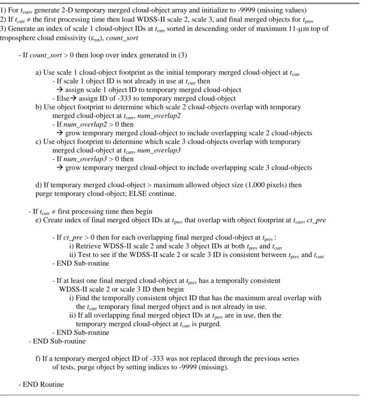
Table 1: Detailed description of main component of the UW-CIMSS post-processing system.

Table 2: Detailed description of the Mature Object Extension option of the UW-CIMSS post-processing system.

Table 3: Detailed description of the Merged-Object Absorption Time option of the UW-CIMSS post-processing system.

Table 4: Mean and standard deviation of the lifetime [mins] of cloud-objects from the

distributions shown in Figure 5. Cloud-objects are binned according to the maximum 11-m top of troposphere cloud emissivity value achieved during their lifetime.

Figure Captions

Figure 1: GOES-12 11-µm brightness temperature (a) and corresponding 11-µm top of troposphere cloud emissivity (b) valid at 2002 UTC 15 May 2009.

Figure 2: High-level flow chart illustrating the procedure of the convective cloud-object tracking system. Section (a) represents the WDSS-II configuration and object building and tracking component of the system. Section (b) represents the post-processing system and Section (c) represents the fusion of multiple meteorological datasets into a single cloud-object framework.

Figure 3: WDSS-II scale 1 (a), scale 2 (b), and scale 3 (c) objects and IDs valid at 2002 UTC 15 May 2009. The final merged cloud-objects and IDs output from the UW-CIMSS post-processing system valid at the same time are shown in panel (d).

Figure 4: 11-µm top of troposphere cloud emissivity (a), final merged cloud-objects and IDs from the UW-CIMSS post-processing system without mature object extension option (b),

merged mature cloud-objects produced by the procedure detailed in Table 2 (c), and final merged cloud-objects and IDs from UW-CIMSS post-processing system with mature object extension applied (d) valid at 2032 UTC 15 May 2009.

Figure 5: Distribution of cloud-object lifetime [mins] as a function of the maximum 11-µm top of troposphere cloud emissivity (tot) achieved during object lifetime. The following tot bins are

shown: 0.2 tot 0.3 (dashed line,---), 0.4 tot 0.5 (dashed circles, -o-), 0.6 tot 0.7 (dashed triangles, -∆-), and tot 0.9 (dashed pluses, -+-).

Figure 6: Cloud-object retention rate as a function of GOES scan interval (a) and as a function of cloud-object size (b). The cloud-object sample size of each group is indicated at the bottom of each bar. Cloud-objects are taken from 34 convectively active periods during 2008 and 2009 over the central and eastern United States and adjacent oceanic regions.

Figure 7: Final merged cloud-objects (a) and the 11-µm top of troposphere cloud emissivity field (b) valid at 2215 UTC 13 May 2009 used as input into the convective cloud-object tracking system. Final cloud-objects are also used in Figure 8 and Figure 9.

Figure 8: Final merged cloud-objects from Fig. 7 (gray contours) valid at 2215 UTC 13 May 2009 are displayed with NEXRAD composite reflectivity (dBZ) (a) and NEXRAD Vertically Integrated Liquid (VIL; kg m-2) (c) valid at 2216 UTC 13 May 2009. Panels (b) and (d) show cloud-objects fused with NEXRAD composite reflectivity and VIL from panels (a) and (c), respectively. The maximum composite reflectivity is shaded in panel (b) for objects that have a valid composite reflectivity, while cloud-objects that have a valid VIL value are shaded

according to their maximum in panel (d).

Figure 9: Final merged cloud-objects from Fig. 7 (gray contours) valid at 2215 UTC 13 May 2009 are displayed with NLDN lightning strikes valid from 2115-2215 UTC 13 May 2009 (a)

May 2009. Panels (b) and (d) show cloud-objects fused with NLDN lightning strike data and RUC MUCAPE from panels (a) and (c), respectively. The elapsed time (mins) from 2215 UTC since an object’s first detected lightning strike is shaded in panel (b), while cloud-objects that have a valid RUC MUCAPE value are shaded according to their maximum in panel (d).

Main Cloud-object Post-processing Procedure

1) For tcurr, generate 2-D temporary merged cloud-object array and initialize to -9999 (missing values) 2) If tcurr the first processing time then load WDSS-II scale 2, scale 3, and final merged objects for tprev 3) Generate an index of scale 1 cloud-object IDs at tcurr sorted in descending order of maximum 11-m top of troposphere cloud emissivity (tot), count_sort

- If count_sort > 0 then loop over index generated in (3)

a) Use scale 1 cloud-object footprint as the initial temporary merged cloud-object at tcurr - If scale 1 object ID is not already in use at tcurr then

 assign scale 1 object ID to temporary merged cloud-object - Else assign ID of -333 to temporary merged cloud-object

b) Use object footprint to determine which scale 2 cloud-objects overlap with temporary merged cloud-object at tcurr, num_overlap2

- If num_overlap2 > 0 then

 grow temporary merged cloud-object to include overlapping scale 2 cloud-objects c) Use object footprint to determine which scale 3 cloud-objects overlap with temporary

merged cloud-object at tcurr, num_overlap3 - If num_overlap3 > 0 then

 grow temporary merged cloud-object to include overlapping scale 3 cloud-objects d) If temporary merged cloud-object > maximum allowed object size (1,000 pixels) then purge temporary cloud-object; ELSE continue.

- If tcurr first processing time then begin

e) Create index of final merged object IDs at tprev that overlap with object footprint at tcurr, ct_pre - If ct_pre > 0 then for each overlapping final merged cloud-object at tprev :

i) Retrieve WDSS-II scale 2 and scale 3 object IDs at both tprev and tcurr

ii) Test to see if the WDSS-II scale 2 or scale 3 ID is consistent between tprev and tcurr - END Sub-routine

- If at least one final merged cloud-object at tprev has a temporally consistent WDSS-II scale 2 or scale 3 ID then begin

i) Find the temporally consistent object ID that has the maximum areal overlap with the tcurr temporary final merged object and is not already in use.

ii) If all overlapping final merged object IDs at tprev are in use, then the temporary merged cloud-object at tcurr is purged.

- END Sub-routine - END Sub-routine

f) If a temporary merged object ID of -333 was not replaced through the previous series of tests, purge object by setting indices to -9999 (missing).

- END Routine

Post-processing Option 1: Mature Object Extension Require: Mature WDSS-II run must be previously processed

1) For tcurr, generate 2-D mature merged cloud-object array and initialize to -9999 (missing values) 2) If tcurr the first processing time then load the final merged objects for tprev and tcurr

3) Generate an index of mature scale 1 cloud-object IDs at tcurr that are smaller than the maximum allowed object size (400 pixels), count_mature

- If count_mature > 0 then loop over index generated in (3)

a) Use mature scale 1 object footprint as the temporary mature merged cloud-object at tcurr b) Use mature object footprint to determine which mature scale 2 cloud-objects overlap

with temporary merged mature cloud-object at tcurr, num_overlap2 - If num_overlap2 > 0 then

 Grow temporary merged mature object to include overlapping mature scale 2 cloud-objects c) Use mature object footprint to determine which mature scale 3 cloud-objects overlap

with temporary merged mature cloud-object at tcurr, num_overlap3 - If num_overlap3 > 0 then

 Grow temporary mature merged object to include overlapping mature scale 3 cloud-objects

d) If temporary merged cloud-object > maximum allowed object size (400 pixels) then purge temporary cloud-object; ELSE continue.

- If tcurr first processing time then begin

e) Test for overlap between temporary mature merged cloud-object at tcurr and any final merged cloud-object at tcurr

- If ‘YES’, skip mature merged object and begin with step 3a for next object index - If ‘NO’, continue to next step

i) Test for overlap between temporary mature merged cloud-object at tcurr and any final merged cloud-object at tprev

- If ‘YES’, skip mature merged object and begin with step 3a for next object in index - If ‘NO’, continue to next step

I) Temporarily insert a new object into the final merged cloud-object field at tcurr that is identical to the mature merged object and,

II) Assign the object ID that corresponds to the final merged object at tprev so long as it has the maximum areal overlap with the merged mature object and is not already used within the final merged cloud-object field at tcurr

- If no such object exists then

 purge the temporary new object from the final merged cloud-object field - END Sub-routine

- END Routine

Table 2. Detailed description of the Mature Object Extension option of the UW-CIMSS post-processing system.

Post-processing Option 2: Merged-Object Absorption Time

1) Generate an index of all final merged objects at tprev that do not exist at tcurr , count_prev - If count_prev > 0 then loop over index generated in (1)

a) Determine the footprint of the final merged cloud-object at tprev b) Check if the object footprint at tprev overlaps with an object at tcurr

i) If ‘YES’, then the final merged object at tprev is assumed to have been absorbed and the absorbed time for the object ID is set to tcurr

ii) If ‘NO’, then the 11-m top of troposphere cloud emissivity (tot) field is sampled at tcurr within the object footprint from tprev. If the maximum tot at tcurr within the tprev object footprint is ≥ 0.50, the object at tcurr is deemed have been purged and the absorbed time for the object ID is set to tcurr

- END Routine

Table 3. Detailed description of the Merged-Object Absorption Time option of the UW-CIMSS post-processing system.

Maximum Object ToT Emissivity (_tot)

Mean Lifetime [mins] StDev [mins]

0.2 _tot 0.3 35.2 37.8 0.4 _tot 0.5 46.8 47.3 0.6 _tot 0.7 91.0 78.1

tot 0.9 155.9 108.3

Table 4. Mean and standard deviation of the lifetime [mins] of cloud-objects from the

distributions shown in Figure 5. Cloud-objects are binned according to the maximum 11-m top of troposphere cloud emissivity value achieved during their lifetime.

Figure 1: GOES-12 11-µm brightness temperature (a) and corresponding 11-µm top of troposphere cloud emissivity (b) valid at 2002 UTC 15 May 2009.

Figure 2: High-level flow chart illustrating the procedure of the convective cloud-object tracking system. Section (a) represents the WDSS-II configuration and object building and tracking component of the system. Section (b) represents the post-processing system and Section (c) represents the fusion of multiple meteorological datasets into a single cloud-object framework.

Figure 3: WDSS-II scale 1 (a), scale 2 (b), and scale 3 (c) objects and IDs valid at 2002 UTC 15 May 2009. The final merged cloud-objects and IDs output from the UW-CIMSS post-processing system valid at the same time are shown in panel (d).

Figure 4: 11-µm top of troposphere cloud emissivity (a), final merged cloud-objects and IDs from the UW-CIMSS post-processing system without mature object extension option (b),

merged mature cloud-objects produced by the procedure detailed in Table 2 (c), and final merged cloud-objects and IDs from UW-CIMSS post-processing system with mature object extension applied (d) valid at 2032 UTC 15 May 2009.

Figure 5: Distribution of cloud-object lifetime [mins] as a function of the maximum 11-µm top of troposphere cloud emissivity (tot) achieved during object lifetime. The following tot bins are shown: 0.2 tot 0.3 (dashed line,---), 0.4 tot 0.5 (dashed circles, -o-), 0.6 tot 0.7 (dashed triangles, -∆-), and tot  0.9 (dashed pluses, -+-).

Figure 6: Cloud-object retention rate as a function of GOES scan interval (a) and as a function of cloud-object size (b). The cloud-object sample size of each group is indicated at the bottom of each bar. Cloud-objects are taken from 34 convectively active periods during 2008 and 2009 over the central and eastern United States and adjacent oceanic regions.

Figure 7: Final merged cloud-objects (a) and the 11-µm top of troposphere cloud emissivity field (b) valid at 2215 UTC 13 May 2009 used as input into the convective cloud-object tracking system. Final cloud-objects are also used in Figure 8 and Figure 9.

Figure 8: Final merged cloud-objects from Fig. 7 (gray contours) valid at 2215 UTC 13 May 2009 are displayed with NEXRAD composite reflectivity (dBZ) (a) and NEXRAD Vertically Integrated Liquid (VIL; kg m-2) (c) valid at 2216 UTC 13 May 2009. Panels (b) and (d) show cloud-objects fused with NEXRAD composite reflectivity and VIL from panels (a) and (c), respectively. The maximum composite reflectivity is shaded in panel (b) for objects that have a valid composite reflectivity, while cloud-objects that have a valid VIL value are shaded

Figure 9: Final merged cloud-objects from Fig. 7 (gray contours) valid at 2215 UTC 13 May 2009 are displayed with NLDN lightning strikes valid from 2115-2215 UTC 13 May 2009 (a) and Rapid Update Cycle Most Unstable CAPE (MUCAPE; J kg-1 K-1) valid at 2200 UTC 13 May 2009. Panels (b) and (d) show cloud-objects fused with NLDN lightning strike data and RUC MUCAPE from panels (a) and (c), respectively. The elapsed time (mins) from 2215 UTC since an object’s first detected lightning strike is shaded in panel (b), while cloud-objects that have a valid RUC MUCAPE value are shaded according to their maximum in panel (d).