A Low Order System Frequency Response
Model for Large Power System and Adaptive
Load Shedding
Kinjal G. Shah
1, Darshit S. Patel
2Assistant Professor, Dept. of EE, Vadodara Institute of Engineering, Vadodara, Gujarat, India 1
Assistant Professor, Dept. of EE, Vadodara Institute of Engineering, Vadodara, Gujarat, India2
ABSTRACT:Now a days electrical system becomes very much large and Power demand will be increasing more and more. To satisfy the power demand nonconventional sources are incorporated in the field of electrical power generation and the system becomes Inter connected. Large power system disturbances sometimes causes interconnected system to become separated into some islands and it has either surplus of generation or load. If generation is more than it can be controlled by controlling the speed of speed governors connected with the generating station will result into change in frequency. This paper includes the derivation of simple low order system frequency response (SFR) model that can be used for estimating the frequency behaviour of the interconnected power system to sudden load disturbances. The SFR model is the simplify model to analyse system dynamics.
KEYWORDS:Frequency, rate of change of frequency, frequency response, governor drop, inertia constant, reheat time constant, regulation.
I.INTRODUCTION
The frequency deviation that accompanies system islanding disturbance is caused by the imbalance between generation and load. The basic concept of model derived here is based on the uniform or average frequency where frequency oscillations or frequency deviation can be filtered out, but the average frequency behaviour retains. There are many theories which can be used to determine the total impedance to “inertial centre” [1, 2, 3], but generally only the generator and transformer impedances are taken in to consideration. The effect of these impedance places a limitation on the amount of load that any generating unit can absorb [4, 5]. SFR model neglects this limitation, assuming that the disturbance is small compared to the total rating of the island, and that the equivalent machine will able to absorb this change.
II.SYSTEM FREQUENCY RESPONSE MODEL
Consider a large system in which most of the generating units are reheat steam turbine units. We require to reduce this system to one described by a minimum number of equations that will use to compute the average frequency behaviour. The dynamic performance of each rotating equipment is controlled by a separate governor by integrating the individual accelerating power.
Fig. 1 Generating Unit Frequency Control
The basic SFR model averages the machine dynamic behaviour in a large system into an equivalent single machine. This approach is to provide the minimum order model that retains the essential average frequency response shape of a system with typical time constants and active speed governing. The simplified model is based on neglecting nonlinearities and allbut the largest time constants in the equations of the generating units of the power system, with assumption that the generation is dominated by the reheat steam turbine generators. This means that the inertia of the generating units and reheat time constants predominate the system average frequency response. The result is a representation of only the average system dynamics, while ignoring the inter-machine oscillations [9]. The dynamic performance of each rotating mass is controlled by a separate governor by integrating the individual accelerating power. A general diagram of an individual power plant is shown in Fig.1
The simplified SFR model of the system is as shown in Fig.2, where all parameters are in per unit on an MVA base equal to the total rating of all generating units. The model behaviour depends on the following factors; the gain, Km , the damping factor ,D, the inertia constant H, the average reheat time constant, TR , and the high pressure power fraction of the reheat turbines, FH. The range of TR is about 6 to 12 seconds and tends to dominate the response of the largest fraction of turbine power output. Therefore we ignore all the time constants. The value of H is on the order of 3 to 6 seconds for a typical large unit and is always multiplied by two, which increases its effect.
Figure 2 Simplified SFR Model Notifications used in this figure are as follows:
H Inertia constant of a generator in per unit second D Damping factor
Km Mechanical power gain factor
TR Reheat time constants in seconds Pd Disturbance power in per unit Pa Accelerating power in per unit
Pm Turbine mechanical power output in per unit
For this system model we compute the frequency response in per unit can be expressed as
Rw
n DRK
m
T
Rs
P
ds
w
nsw
n
w 2/ 1 / 22 2
(1) Where,
T
K
w
n DR m/2HR R2
2HR DRK
mF
HT
R/2DRK
m
/w
n
and the per unit speed or frequency can be computed for and disturbance power. For sudden disturbances, large or small, we are usually interested in disturbance power in the form of a step function Pstepwhich change equation (1) into the following form
Rw
n DRK
m
T
Rs
P
step s
s
w
nsw
n
w 2/ 1 / 22 2
(2)
P
K
e
t t
m step w w DR R t
w n r
sin
1
/ (3)
Where,
2 2 2
1 / 2
1
T
Rw
nT
Rw
n
21
w
w
r n
2 1
w
rT
R w
nT
R
1 /tan
1 1
1 22 tan 1
Here we are using SFR model to calculate PL
, which is defined as the maximum amount of power mismatch (in p.u.) between the generation and load, for which the frequency does not fall below a present value. The study considers this value of the frequency as 58 Hz in 60 Hz system and 48 Hz in a 50 Hz system.III.RESULT AND DISCUSSION
under frequency load shedding by the following example. For that we have assumed the largest disturbance to be a sudden maximum disturbance at 100 % of the total generation of the system. The curves of disturbances up to and including this 1.0 p.u. disturbance are shown in Fig. 3. We also observe that no load shedding is required for disturbances smaller than 0.4 per unit as these disturbances do not cause the frequency to fall below the 57 Hz threshold.
Fig. 3 Frequency Response to Load Disturbance
The average system parameters for this example are as follows: Km = 0.85, FH = 0.3, D = 1.0, TR = 8.0, H = 3.5, R = 0.06
Table shows the computed initial slope and maximum frequency deviation for the typical system condition.
PStep (p.u.) m0 (p.u. / s) Δωmax (Hz) fmin(Hz)
-0.2000 -0.0286 -1.6438 58.356
-0.3648 -0.0521 -3.0000 57.000
-0.4000 -0.0521 -3.2876 56.712
-0.6000 -0.0857 -5.1429 55.069
-0.8000 -0.1143 -6.5751 53.425
-1.0000 -0.1429 -8.2189 51.781
Table I Initial Slope and Maximum Deviation
The second row of Table represents the maximum step change of load that can be permitted if the frequency is not to decline below 57 Hz. Therefore, when the magnitude of the observed initial slope is greater than 0.0521 p.u. /s, load shedding must be triggered. Note that the initial slope for -0.3648 p.u. step disturbance is -0.0521 p.u. /s. So the load that must be shed by subtracting 0.0521 per unit/s from the computed slope for any disturbance. The size of the disturbance is the initial slope of frequency decline. This slope equal to
𝑚0= 60 ∗ 𝑑𝛥𝜔
𝑑𝑡 =
60∗𝑃𝑆𝑡𝑒𝑝
2∗𝐻 𝐻𝑧 𝑠𝑒𝑐 (4)
𝑃𝑆𝑡𝑒𝑝 = 2∗𝐻∗𝑚0
60 𝑝𝑒𝑟𝑢𝑛𝑖𝑡
(5)
The load shedding plan use a time delay of 0.1 sec. or 6 cycles, for each load shedding step. It is important to detect the need for shedding very quickly and to complete all load shedding before the frequency can decay to hazardous level. The load shedding is initiated at about 0.1 seconds after the disturbance, with the first step of load shed after 0.1 second time delay, or at about 0.2 seconds. Therefore, the incremental load shed should be equal to the following.
𝑃𝑠ℎ 𝑒𝑑
2𝐻 =
𝑃𝑠𝑡𝑒𝑝
2𝐻 − 0.0521 𝑝.𝑢. 𝑠𝑒𝑐 (6)
Solving for Pshed and substitution in equation (5) for the step change, we compute,
Pshed = Pstep - 0.1042*H = H*(m0/30 - 0.1042) p.u. (7)
From this equation, we may compute the incremental step function of load to be shed for various sizes of the initial disturbances. The amount of load shed in per unit is a function of only the inertia constant and the observed slope. The initial slope is the only unknown in equation (7). This initial slope contains all the information required to estimate the size of the step change in load caused by the system separation and to forecast the depth and even the approximate time of the maximum frequency dip. The amount of load to be shed is determined from equation (7). The result of load shed values and frequencies are as shown in table below.
Frequency (Hz) Amount of Load Shed (p.u.)
59.5 0.317
59.2 0.10
58.9 0.10
58.6 0.10
58.3 0.05
Total load shed 0.667
Table II Load Shed Schedule for 1.0 per Unit Step
Using the load shedding steps shown in Table II and the given system parameters, the frequency response is computed using the SFR model. The result is shown in Fig. 4. It is very difficult to visualize the effect of each physical parameter of the SFR model without plotting the results. So, the each parameter is now varied and the results plotted to illustrate the effect of that parameters.
The effect of Governor Droop, R
The value of R is varied from 0.05 to 0.10 in the increment of 0.01 per unit. The results are shown in Fig.5. It is observed that the assumed droop setting R has no effect on the initial rate of frequency decline.
Fig. 5 Frequency Response for varying value of R
The effect of Inertia, H
The value of H has a direct effect on the initial slope, as shown in the Fig.6 for various H values. The inertia constant affects the values of ωn and ξ and also on the initial slope and the time of the peak response.
Fig. 6 Frequency Response for varying value of H
The effect of Reheat Time Constant, TR
Fig. 7 Frequency Response for varying value of TR
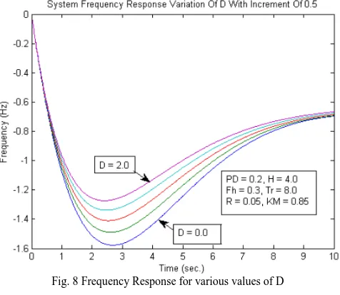
The effect of Frequency Dependence of Load
Power system loads are known to be sensitive to system frequency. The incremental change in load is a function of the incremental change in frequency. But this effect is included in the model in the form of the damping constant D, so we can write,
ΔPL = DΔω (8)
Where all values are in per unit. The system undamped natural frequency and damping are function of D, but this dependence is appears as the product of DR. Since R is small, nominally about 0.05 per unit, the product DR will be small and the effect of D is dismissed. The effect on the frequency response with varying D is as shown in Fig.8. It is observed that the plot is similar to Fig.5 but with the reduced effect.
Fig. 8 Frequency Response for various values of D
IV.CONCLUSION
described for determining the amount of load to be shed by under frequency load shedding method based on the initial slope calculation. This initial slope contains all the information required to estimate the size of the step change in load caused by the system disturbance. From this observation, the first step of load shedding can be set up adaptively, with additional steps to follow at prescribed intervals and amount. The first step is considered the most important and is selected arbitrarily at one half the static load shed target, with additional increments of about 0.1 per unit to be shed at 0.3 Hz increments until the dynamic load shed amount has been reached.
REFERENCES
[1]C. Tavora and 0. J. M. Smith, "Stability Analysis of Power Systems, Report ERL-70-5, College of Engineering, University of California, 1970.
[2] K. N. Stanton, "Dynamic Energy Balance Studies for Simulation of Power Frequency Transients," Proc PICA Conference, IEEE PES, C26-PWR,
1971.
[3] P. M. Anderson and A. A. Fouad, Power System Control and Stability, Iowa State University Press,Ames, 1978.
[4] M. S. Baldwin, M. M. Merrian, H. S. Schenkel, and D. J. VandeWalle, "An Evaluation of Loss of Flow Accidents Caused by Power System
Frequency Transients in Westinghouse PWR's, Westinghouse Report WCAP-8424, May 1975.
[5] M. S. Baldwin and H. S. Schenkel, "Determination of Frequency Decay Rates During Periods of Generation Deficiency," IEEE Trans.,v PAS-95, n 1,\ Jan/F'eb 1976.
[6] P.M. Anderson and M. mirheydar, " An adaptive method for setting under frequency load shedding relays, " IEEE Trans. on Power Systems, vol.
7, no. 2, may 1992, pp. 647-655.
[7] P.kundur, Power System Stability & Control, ser. Power System Engineering Series, Newyork : Mc Graw hill, 1994.
[8] P.M. Anderson and M.Mirheydar, " A low order system frequency response model," IEEE Trans. on Power Systems, vol.5, no.3, August 1990,
pp.720-729.
BIOGRAPHY
Kinjal G. Shah received the B.E. Degree in Electrical Engineering From A.D. Patel Institute Of Technology, V.V.Nagar , Gujarat, India in 2011 and M.Tech degree in Electrical Power System from Charutar University Of Science and Technology, CHARUSAT, Changa, Gujarat,India in 2013.She is currently an Assistant Professor in the Department of Electrical Engineering, Vadodara Institute Of Engineering, Vadodara, Gujarat. Her research interests include electrical machines, wide area monitoring systems, voltage stability assessment and control.