Novel Control of PV Solar and Wind Farm Inverters as STATCOM for Increasing Connectivity of Distributed Generators

(1)

Scholarship@Western

Electronic Thesis and Dissertation Repository

4-23-2013 12:00 AM

Novel Control of PV Solar and Wind Farm Inverters as STATCOM

for Increasing Connectivity of Distributed Generators

Mahendra AC

The University of Western Ontario

Supervisor

Dr. Rajiv K. Varma

The University of Western Ontario

Graduate Program in Electrical and Computer Engineering

A thesis submitted in partial fulfillment of the requirements for the degree in Master of Engineering Science

Follow this and additional works at: https://ir.lib.uwo.ca/etd

Part of the Power and Energy Commons

Recommended Citation Recommended Citation

AC, Mahendra, "Novel Control of PV Solar and Wind Farm Inverters as STATCOM for Increasing Connectivity of Distributed Generators" (2013). Electronic Thesis and Dissertation Repository. 1241.

https://ir.lib.uwo.ca/etd/1241

This Dissertation/Thesis is brought to you for free and open access by Scholarship@Western. It has been accepted for inclusion in Electronic Thesis and Dissertation Repository by an authorized administrator of

(2)

NOVEL CONTROL OF PV SOLAR AND WIND FARM INVERTERS AS STATCOM FOR INCREASING CONNECTIVITY OF DISTRIBUTED GENERATORS

(Thesis format: Monograph Article)

by

Mahendra AC

Graduate Program in Engineering Science

Department of Electrical and Computer Engineering

A thesis submitted in partial fulfillment of the requirements for the degree of

Master of Engineering Science

The School of Graduate and Postdoctoral Studies The University of Western Ontario

London, Ontario, Canada

(3)

ii

ABSTRACT

The integration of distributed generators (DGs) such as wind farms and PV solar farms in

distribution networks is getting severely constrained due to problems of steady state voltage

rise and temporary overvoltages (TOV). This thesis presents a first time application of a

patent-pending PV solar farm control as a dynamic reactive power compensator

(STATCOM), termed PV-STATCOM, for mitigating the voltage rise and TOV issues, and

significantly enhancing the connectivity of a neighbouring wind farm both during night and

day in a realistic distribution feeder in Ontario. The effectiveness of PV-STATCOM is

demonstrated even if the solar farm is located 30 km away from wind farm on a common

distribution line. The PV-STATCOM utilizes the entire inverter capacity in the nighttime and

the inverter capacity remaining after solar power generation during daytime. A novel control

of full converter based wind farm as Wind-STATCOM for substantially increasing the

connectivity of a neighbouring PV solar farm is also described. The Wind-STATCOM

employs the inverter capacity left after that needed for wind power production, both during

night and day. Subsequently, a new combined application of PV-STATCOM and

Wind-STATCOM to improve the connectivities of both solar farm and wind farm to significantly

high levels in a common distribution feeder is presented. These studies have been conducted

for the first time in known literature. Commercial grade software PSS/E and

PSCAD/EMTDC are used to evaluate the steady state voltage profile and TOVs,

respectively, in distribution feeder having different Reactance (X) /Resistance (R) ratios.

Keywords:

Distributed Generator (DG), Static Synchronous Compensator (STATCOM), Photovoltaic

(4)

iii

Dedicated to

(5)

iv

ACKNOWLEDGMENTS

I would like to express my sincere gratitude to my thesis supervisor Prof. Rajiv K. Varma for

his persistent support and utmost guidance in my research work. His broad knowledge and

thoughtfulness has been a constant source of motivation for hard work and sincerity.

I would like to acknowledge the financial support provided by the University of Western

Ontario and Natural Sciences and Engineering Research Council of Canada (NSERC). I am

also grateful to the faculty and administrative staff of the department for their contribution

and support throughout my study at Western.

I express my gratitude towards my friends Akshaya, Arif, Ehsan, Byomakesh and Gagan for

their constructive suggestions, excellent company and constant support.

(6)

v

LIST OF TABLES

Table 2.1 Study system bus identification ... 21

Table 3.1 Base case steady state analysis - Voltages at various nodes of the system for

daytime and nighttime ... 60

Table 3.2 Steady state results for daytime loading, Case 1: 0% Solar farm output,

PSF = 0.0 MW, QSF = 0.0 Mvar ... 63

PSF = 4.25 MW, QSF = 0.0 Mvar ... 64

PSF = 8.5 MW, QSF = 0.0 Mvar ... 64

Table 3.5 Steady state results for nighttime loading, PSF = 0.0 MW, QSF = 0.0 Mvar ... 65

Table 3.6 Steady state voltages with reactive power compensation during daytime

Case 1: 0% solar farm output, PSF = 0.0 MW ... 71

Table 3.9 Steady state voltages with reactive power compensation

Nighttime loading: PSF = 0.0 MW ... 72

Table 3.10 Base case steady state voltages with X/R ratio variation ... 78

Table 3.11 Base case results for X/R ratio variation, PSF = 0.0 MW, PWF = 0.0 MW ... 82

Table 3.12 Steady state voltages with X/R ratio variation for daytime

(12)

xi

Table 3.15 Steady state voltages with X/R ratio variation for nighttime,

PSF = 0.0 MW ... 85

Table 3.16 Summarized results for wind farm connectivity ... 86

Table 4.1 Steady state voltage for daytime loading Case 1: 0% wind farm output,

PWF = 0.0 MW, QWF = 0.0 Mvar ... 95

PWF = 4.95 MW, QWF = 0.0 Mvar ... 95

PWF = 9.9 MW, QWF = 0.0 Mvar ... 95

Table 4.4 Steady state voltages with reactive power compensation from Wind-STATCOM,

Case 1: 0% wind farm output PWF = 0.0 MW ... 99

Case 2: 50% wind farm output PWF = 4.95 MW ... 99

Case 3: 99% wind farm output PWF = 9.8 MW ... 99

Table 4.7 Steady state voltages with X/R ratio variation – without and with

Wind-STATCOM, Case 1: 0% wind farm output PWF = 0.0 MW ... 101

Table 4.8 Steady state voltages with X/R ratio variation – with and without

Wind-STATCOM, Case 2: 50% wind farm output PWF = 4.95 MW ... 102

Table 4.9 Steady state voltages with X/R ratio variation – with and without

(13)

xii

Table 4.10 Summarized results for solar farm connectivity ... 104

Table 5.1 Steady state voltages for daytime loading ... 107

Table 5.2 Steady state voltages for nighttime loading ... 108

Table 5.3 Steady-state voltages with reactive power compensation using PV-STATCOM

(Daytime loading, Solar farm output, PSF = 20.0 MW ) ... 113

Table 5.4 Steady-state voltages with reactive power compensation using Wind-STATCOM

(14)

xiii

LIST OF FIGURES

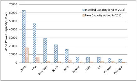
Figure 1.1 Total installed capacity (end of 2011) and new capacity added in 2011 for top 10

wind power producing countries ... 2

Figure 1.2 Growth of wind generation installed capacity in Canada ... 2

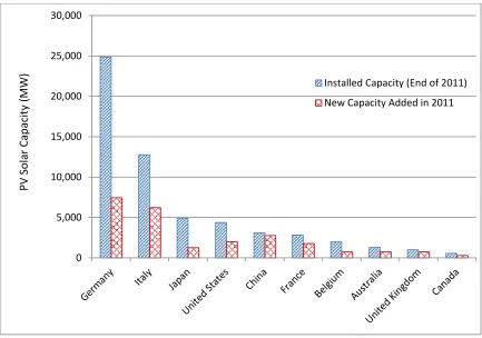
Figure 1.3 Total installed capacity (end of 2011) and new capacity added in 2011 for top 10 solar power producing countries ... 3

Figure 1.4 Growth of PV solar installed capacity in Canada ... 3

Figure 1.5 Radial distribution system with DG ... 5

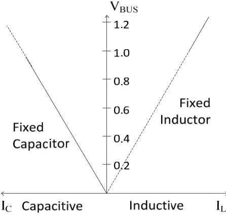
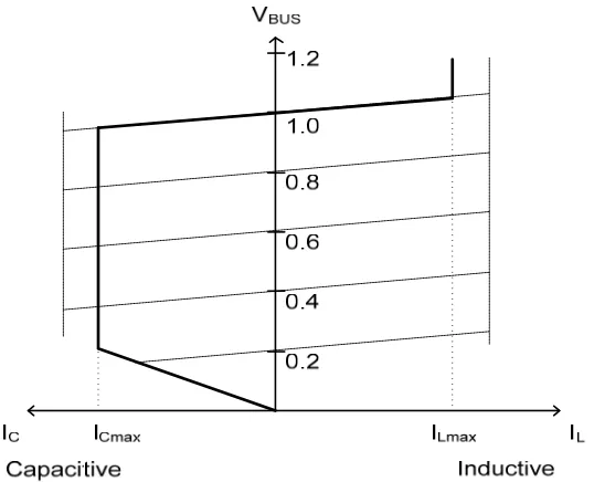
Figure 1.6 Terminal characteristic of fixed Capacitor/Inductor ... 8

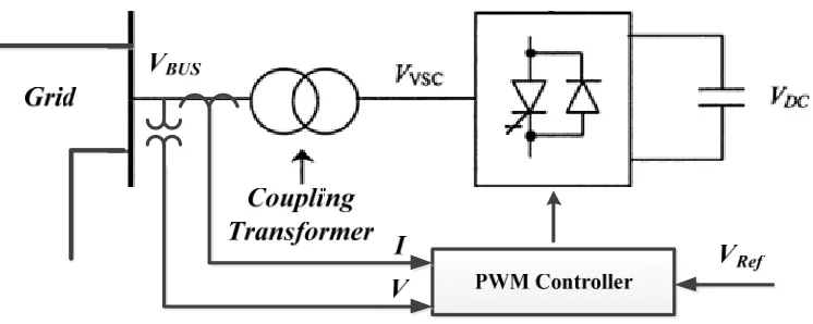
Figure 1.7 STATCOM connected to AC system through coupling transformer ... 10

Figure 1.8 Terminal characteristic for a STATCOM ... 11

Figure 1.9 Single line representation of STATCOM terminal connected to the grid ... 11

Figure 1.10 Phasor diagram showing reactive power control by STATCOM, (a) Reactive power consumed by STATCOM – Inductive mode, and (b) Reactive power supplied by STATCOM – Capacitive mode ... 12

Figure 1.11 Phasor diagram showing active power control by STATCOM - (a) Active power consumed by STATCOM – Power flow from AC to DC side (b) Active power supplied by STATCOM – Power flow from DC to AC side .. 12

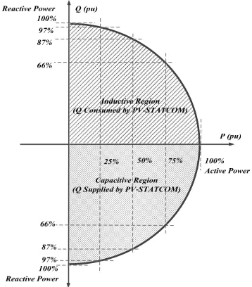
Figure 1.12 Active/reactive power capability curve for PV-STATCOM ... 15

Figure 2.1 Study system ... 21

Figure 2.2 Grid modeled as voltage source with equivalent impedance ... 22

(15)

xiv

Figure 2.4 Equivalent -model of overhead line (lumped parameters) ... 24

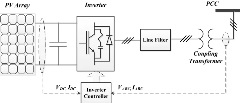
Figure 2.5 PV Solar System ... 26

Figure 2.6 Equivalent circuit of PV solar cell ... 27

Figure 2.7 A typical current-voltage characteristic of PV module ... 29

Figure 2.8 Schematic diagram of LC filter and coupling transformer ... 31

Figure 2.9 Generation of sinusoidal reference signal (for firing pulse generation for SPWM control) ... 34

Figure 2.10 Generation of triangular reference signal (for PWM control) ... 35

Figure 2.11 STATCOM voltage control with 3% droop characteristics ... 36

Figure 2.12 Phase shift angle control to maintain real power transfer ... 36

Figure 2.13 DC side voltage control with real power transfer ... 37

Figure 2.14 Voltage control strategy for unbalanced fault conditions ... 38

Figure 2.15 Study system model with PV-STATCOM (PSCAD/EMTDC model) ... 39

Figure 2.16 Step response with variation of proportional gain, Kp Case 1: PSF = 0.0 MW ... 40

Figure 2.17 Step response with variation of integral time constant, Ti Case 1, PSF = 0.0 MW ... 41

Figure 2.18 Step response with variation of proportional gain, Kp Case 2, PSF = 5.0 MW ... 42

Figure 2.19 Step response with variation of integral time constant , Ti Case 2, PSF = 5.0 MW ... 42

(16)

xv

Figure 2.21 PCC voltage control with PV-STATCOM: Case 2, Daytime loading with

PSF = 5.0 MW and PWF = 10.0 MW ... 45

Figure 2.22 Phase voltages without and with PV-STATCOM for single line to ground fault (SLGF) for 0.1 sec. ... 47

Figure 2.23 Schematic representation of typical wind turbine system ... 47

Figure 2.24 Induction Generator based wind turbine generator (fixed speed operation) ... 48

Figure 2.25 Stator and rotor representation of induction machine ... 49

Figure 2.26 Per-phase equivalent circuit model of induction machine ... 50

Figure 2.27 Permanent Magnet Synchronous Generator (PMSG) based wind turbine (variable speed operation) ... 51

Figure 2.28 Wind turbine and rectifier control schemes ... 53

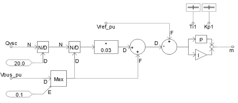
Figure 2.29 Schematic diagram of Wind-STATCOM control ... 54

Figure 2.30 PSCAD/EMTDC model of the study system with Wind-STATCOM ... 56

Figure 2.31 PSS/E model of the complete system ... 57

Figure 3.1 Study system with PV-STATCOM ... 59

Figure 3.2 Base case voltages at various buses for daytime and nighttime ... 61

Figure 3.3 Phase voltages for daytime loading with single line to ground fault ... 61

Figure 3.4 Phase voltages for nighttime loading with single line to ground fault ... 62

Figure 3.5 PCC bus voltages for various solar farm output cases with increasing wind farm output (daytime and nighttime) ... 66

(17)

xvi

Figure 3.7 Phase voltages for daytime loading with SLGF

Case 1: PSF = 0.0 MW, PWF = 11.5 MW ... 67

Figure 3.8 Phase voltages for daytime loading with SLGF Case 2: PSF = 4.25 MW, PWF = 5.4 MW ... 68

Figure 3.9 Phase voltages for daytime loading with SLGF Case 3: PSF = 8.33 MW, PWF = 2.1 MW ... 68

Figure 3.10 Phase voltages for nighttime loading with SLGF, PSF = 0.0 MW, PWF = 20.0 MW ... 69

Figure 3.11 Phase voltages for nighttime loading with SLGF, PSF = 0.0MW, PWF = 3.9 MW ... 69

Figure 3.12 Phase voltages for daytime loading with SLGF, PSF = 0.0 MW, PWF = 19.5 MW ... 73

Figure 3.13 Phase voltages for nighttime loading with SLGF, PSF = 0.0 MW, PWF = 16.6 MW ... 74

Figure 3.14 Annual sunshine graph for London, Ontario (Source: www.gaisma.com) ... 75

Figure 3.15 Available active and reactive power capacity for solar farm converter based on typical insolation (approximate sunshine data) and PV module output ... 76

Figure 3.16 Reactive power compensation provided by solar farm (PV-STATCOM) to maintain PCC voltages within permissible limits (±6%) ... 76

Figure 3.17 Maximum reactive power compensation provided by PV-STATCOM to maintain steady-state voltage within permissible limits ... 77

Figure 3.18 PCC voltages for base case with X/R ratio variation ... 79

Figure 3.19 Phase voltages for SLGF Daytime base case loading: Half X/R (1.236) ... 80

(18)

xvii

Figure 3.21 Phase voltages for SLGF Nighttime base case loading: Half X/R (1.236) ... 81

Figure 3.22 Phase voltages for SLGF Nighttime base case - Double X/R (4.994) ... 81

Figure 3.23 Increase in wind farm connectivity with solar farm inverter as PV-STATCOM87 Figure 3.24 Increase in wind farm connectivity with PV-STATCOM (No reactive power compensation available during peak irradiance) ... 88

Figure 4.1 Study system with Wind-STATCOM ... 91

Figure 4.2 Base case steady state voltage profile for PLD = 4.82 MW, QLD = 2.19 Mvar ... 92

Figure 4.3 Phase voltages for daytime loading with SLGF ... 93

Figure 4.4 PCC bus voltages for various wind farm output cases with increasing solar farm output (Daytime loading without compensation) ... 96

Figure 4.5 Phase voltages for daytime loading with SLGF, Case 1: PWF = 0.0 MW,PSF = 20.0 MW... 97

Figure 4.6 Phase voltages for daytime loading with SLGF, Case 2: PWF = 4.95 MW, PSF = 20.0 MW... 97

Figure 4.7 Phase voltages for daytime loading with SLGF, Case 3: PWF = 9.9 MW,PSF = 20.0 MW... 98

Figure 4.8 Reactive power compensation provided by Wind-STATCOM to maintain PCC voltages within permissible limits (0.94 pu – 1.06 pu) ... 100

Figure 5.1 Phase voltages for daytime loading with SLGF, PSF = 8.5 MW, PWF = 9.9 MW ... 109

Figure 5.2 Phase voltages for nighttime loading with SLGF, PSF = 0.0 MW, PWF = 9.9 MW ... 109

(19)

xviii

Figure 5.4 Steady-state voltage profile at wind farm PCC (Nighttime loading) ... 111

Figure 5.5 Phase voltages for daytime loading with SLGF,

PSF = 20.0 MW, PWF = 20.0 MW ... 112

Figure 5.6 Phase voltages for nighttime loading with SLGF,

(20)

xix

LIST OF ABBREVIATIONS

ALFC : Automatic Load Frequency Controller

AVR : Automatic Voltage Regulator

CBEMA : Computer and Business Equipment Manufacturer’s Association

CSC : Current Sourced Converter

DER : Distributed Energy Resources

DFIG : Doubly Fed Induction Generator

DG : Distributed Generation/Distributed Generator

DR : Distributed Resources

EMTDC : Electromagnetic Transients including DC

EPS : Electric Power System

FACTS : Flexible AC Transmission Systems

FIT : Feed-In Tariff

GTO : Gate Turn-off Thyristor

HONI : Hydro One Networks Inc.

HV : High Voltage

IGBT : Insulated Gate Bipolar Transistor

ITIC : Information Technology Industry Council

LV : Low Voltage

MPPT : Maximum Power Point Tracking

MV : Medium Voltage

OLTC : On Load Tap Changer

PCC : Point of Common Coupling

(21)

xx PLL : Phase Locked Loop

PMSG : Permanent Magnet Synchronous Generator

PSCAD : Power Systems Computer Aided Design

PSS/E : Power System Simulator for Engineers

PWM : Pulse Width Modulation

PV : Photovoltaic

PV-STATCOM : Photovoltaic (Inverter) Static Synchronous Compensator

SCIG : Squirrel Cage Induction Generator

SEIG : Self-Excited Induction Generator

SLGF : Single Line to Ground Fault

SPWM : Sinusoidal Pulse Width Modulation

STATCOM : Static Synchronous Compensator

SVC : Static Var Compensator

TOV : Temporary Overvoltage

VSC : Voltage Sourced Converter

Wind-STATCOM : Wind turbine (Inverter) Static Synchronous Compensator

WRSG : Wound Rotor Synchronous Generator

(22)

xxi

LIST OF SYMBOLS

PLD : Active power consumed by load

QLD : Reactive power consumed by load

PSF : Active power supplied by solar farm

QSF : Reactive power compensation by solar farm

Positive - Inductive mode (consumed by solar farm), Negative - Capacitive mode (Supplied by solar farm)

PWF : Active power supplied by wind farm

QWF : Reactive power compensation by wind farm

Positive - Inductive mode (consumed by wind farm), Negative - Capacitive mode (Supplied by wind farm)

Vbus1 : Voltage magnitude at Bus 1 (in pu)

(23)

Chapter 1

1 INTRODUCTION

1.1 Growth of Wind Power and PV Solar Power Based

Distributed Generators

Solar farms and wind farms are the most common distributed generators (DGs) that are

primarily being connected in power distribution networks worldwide [1], [2]. By the end

of 2012 global wind energy installed capacity increased to 276,055 MW, which was a

significant growth from 4,800 MW in 1995 with average cumulative annual growth rate

of about 28.5% [3]. The total installed capacity of the world’s major wind power

producing countries is shown in Figure 1.1 whereas, the growth of wind power in Canada

is given in Figure 1.2.

Due to incentives provided by several governments, small and medium scale PV solar

installations are being increasingly installed worldwide [4]. Feed-in Tariff (FIT) program

implemented by Ontario Government has helped to boost the growth of PV solar farm

and wind farm in Ontario. The worldwide installations of PV solar capacity is shown in

(24)

2

Figure 1.1 Total installed capacity (end of 2011) and new capacity added in 2011 for top 10 wind power producing countries

Figure 1.2 Growth of wind generation installed capacity in Canada

0 10000 20000 30000 40000 50000 60000 70000

Installed Capacity (End of 2011)

New Capacity Added in 2011

Wind Power Capacity (MW)

137 198 236 322

444 684 1,460 1,846 2,369 3,319 4,008 5,511 0 500 1000 1500 2000 2500 3000 3500 4000 4500 5000 5500 6000

2000 2001 2002 2003 2004 2005 2006 2007 2008 2009 2010 June 2012

(25)

Figure 1.3 Total installed capacity (end of 2011) and new capacity added in 2011 for top 10 solar power producing countries

Figure 1.4 Growth of PV solar installed capacity in Canada

0 5,000 10,000 15,000 20,000 25,000 30,000

Installed Capacity (End of 2011)

New Capacity Added in 2011

PV Solar Capacity (MW) 0 50 100 150 200 250 300 350

2000 2001 2002 2003 2004 2005 2006 2007 2008 2009 2010

Off-grid

Grid Connected Total

Cumulative PV Solar Installation in Canada

(as of December 31 of each year)

Installed

C

apacity

(26)

4

1.2 Issues with Grid Integration of DGs

Traditionally, power grids are fed from large centralized generating stations mainly based

on hydro, thermal or nuclear generation technologies. The integrated power grids are

characterized by large generation, bulk transmission and end use through distribution

network. However, the distributed nature of renewable energy resources like solar and

wind have transformed this traditional integrated power network with presence of a large

number of small scale distributed generators (DGs) [5] . These distributed generators are

normally connected to the medium voltage (MV) and low voltage (LV) distribution

networks.

The interconnection of DGs in distribution network provides additional benefits in the

network. With the development of solar farm and wind farm in medium voltage

distribution network, the increase in the demand can be locally fulfilled reducing the cost

of transmission network expansion. It also helps to reduce the transmission congestion in

existing network. The transmission and distribution losses are reduced increasing the

system efficiency. However, these benefits come along with new challenges to the system

operator. The major issues encountered by the medium voltage distribution with the

integration of distributed generation include, but not limited to, steady state voltage rise,

increased temporary overvoltage (TOV), increase in voltage flicker and harmonic

components, and restrictions on operation of existing grid protection [5] – [7] .

1.2.1 Steady state voltages

Connecting the DGs towards the receiving end of radial distribution system may create

reverse power flow during the light load condition (off-peak load during nighttime). In

this situation, the distribution line, traditionally operated to carry designed amount of

power from the source end towards the load end, is likely to face increased voltage at the

receiving end due to reverse power flow [6]. A typical scenario of reverse power flow can

occur when DG output is greater than the load for the distribution network, shown in

(27)

Figure 1.5 Radial distribution system with DG

For this network, the receiving end voltage is given by:

∙ ∙ ……… 1.1

where, ∙ /

,

∙ / ∙ ∙

, ∙ ∙ / ∙ ∙ ∙ / … 1.2

The approximate expression for receiving end voltage is:

∙ ∙ / ……… 1.3

For the DG in the receiving end with active power injection of at unity power factor,

the receiving end voltage is given by:

∙ ∙ / ……… 1.4

From this expression we can identify that the receiving end voltage will increase

(28)

6

generation at receiving end and the line resistance . For a distribution

system with low X/R ratio (i.e. high line resistance R), the rise in voltage can be

substantial.

The guidelines provided by IEEE Standards (IEEE Std 1547-2003: IEEE Standard for

Interconnecting Distributed Resources with Electric Power Systems) [8] – [10] and CSA

Standards (CSA C22.3 No. 9-08: Interconnection of distributed resources and electricity

supply systems) [11] are widely implemented to specify the permissible steady-state

voltage variation in distribution network. The steady state voltage limit of ±6% of

nominal value at the end user terminal is permitted in Hydro One’s Technical

Interconnection Requirements [7]. Appropriate reactive power compensation is required

to maintain steady state voltage within permissible limits. The conventional mitigation

measures for voltage issues are discussed in Section 1.3 whereas measures based on

Flexible AC Transmission Systems (FACTS) are discussed in Section 1.4.

1.2.2 Temporary

overvoltage

In medium voltage networks, unbalanced faults, such as single line to ground fault

(SLGF) in the network causes temporary overvoltages (TOV) on the healthy phases of

the network feeder [12], [13]. Overvoltages between one phase and ground or between

two phases are classified based on the shape of the voltage, percentage increase from

nominal value and duration of application. Temporary overvoltages (TOV) originating

from switching or system faults (e.g. load rejection, unbalanced faults) or from

nonlinearities (ferroresonance effects, harmonics) are normally undamped or weakly

damped [10].

Integration of distributed generators causes changes in fault level, fault current

distribution and voltage profile in the distribution line. TOV in the distribution line

mainly depends on pre-fault voltage, type of fault, fault resistance, etc. Single line to

ground bolted fault is considered to observe the impact of temporary overvoltage in this

thesis. The types of distributed generator and configuration of its interconnection

(29)

The range of higher and lower level of system voltages, that end user equipment can

safely handle, are specified by CBEMA voltage curves [14]. These characteristic shows

that the voltage level as well as the time interval for which such voltages appear are both

important in identifying the level of acceptable temporary overvoltage. The temporary

rises in voltage are specified by IEEE standards [8] and CSA standards [11]. Based on

these requirements, Hydro One Networks Inc. has specified that the TOV anywhere in

the distribution network under no circumstances shall exceed 130% [7].

1.3 Conventional Mitigation Measures for Voltage Issues

In any power network, voltages at various system buses change continuously according

to the variation in demand, switching of lines and transformers, and system

contingencies. Power system operators are responsible for maintaining system voltages

within permissible limits in all operating conditions. Typically, on load tap changing

(OLTC) transformers are used to maintain voltages in medium voltage distribution

network.

1.3.1 Voltage

Regulation

Voltage control is achieved by implementing voltage regulators [15] at various locations

in power network. Most of the existing voltage regulators in the distribution network are

implemented for unidirectional power flow from the source to the load ends. Increased

DG output during off-peak load hours, may result in reverse power flows. The upstream

voltage regulators are affected by such reverse power flow [15]. Modifications of the

controller have been proposed for the upstream line voltage regulators if DGs are

connected to the system. Multiple line drop compensation based voltage regulators are

effective to regulate the system voltage even with high penetration of distributed

generators [16]. In the traditional distribution system, the system voltage is maintained by

implementing upstream voltage regulators and the load end reactive power compensators.

(30)

8

1.3.2 Reactive

Power

Compensation

It is a well-known fact that shunt compensation can be used to provide reactive power

compensation locally at load buses. Conventional shunt capacitors or shunt inductors are

used for this purpose. Capacitive reactive power compensation is used to increase the

system voltage to desired level where as inductive compensation is used to reduce the

voltage during light load (off-peak) conditions. The terminal characteristic (I-V

characteristic) for fixed capacitor and inductor is shown in Figure 1.6.

Shunt capacitors and inductors provide fixed compensation. Variable compensation is

implemented by switching appropriate combination of capacitors or inductors. The

variability of distributed generation resources and requirement of dynamic reactive power

support make these conventional devices less effective in resolving voltage issues created

by DGs. Synchronous condensers can provide continuously controlled reactive power

output from inductive to capacitive region [17]. However, such devices have slow

response and are less commonly employed in distribution systems due to their high cost.

(31)

1.4 FACTS Controller based Mitigation Measures for

Voltage Issues

Flexible AC Transmission System (FACTS) is defined as the AC transmission systems

incorporating power electronics based and other static controllers to enhance

controllability and increase power transfer capability [18]. The FACTS Controllers

impart the following benefits to the electric power network:

 Provides reactive power compensation

 Provides voltage regulation

 Improves steady-state stability and transient stability

 Damps power system oscillations

 Improves voltage stability

 Increases power transfer capability

In medium voltage distribution networks, shunt FACTS devices are used to provide very

fast and continuous reactive power support. It helps to improve system power factor and

regulate the system voltage. Due to their fast response and dynamic reactive power

support capability, FACTS Controllers are most suitable to mitigate voltage fluctuation

created by the solar and wind power integration to the grid [19]. Mostly, Static Var

Compensator (SVC) – a thyristor based FACTS Controller [17], [20] and Static

Synchronous Compensator (STATCOM) – a voltage source converter based FACTS

Controller are used in medium voltage distribution network.

1.4.1 Static Synchronous Compensators (STATCOM)

The Static Synchronous Compensator (STATCOM) is a FACTS Controller utilized at the

transmission and distribution level [18], and as a custom power device at end users’

electrical installations [21]. The major applications of STATCOM in these contexts

include voltage regulation, power factor correction, damping power oscillations, and load

(32)

10

1.4.1.1 Principle

of

Operation

Static synchronous compensator (STATCOM) is a voltage sourced converter (VSC)

based on controllable switches. A STATCOM is a shunt connected device that provides

rapid reactive power compensation in the network.

STATCOM, which injects sinusoidal current at the point of common coupling, can

emulate itself as inductive or capacitive reactive power source by aligning the injected

current almost in quadrature with line voltage [22], [23]. A STATCOM with proper

control strategy can be effectively used to suppress voltage fluctuation in the network

[24], [25], [26].

A functional representation of the STATCOM showing various components is shown in

Figure 1.7. The STATCOM is connected to the AC system terminal bus through a

coupling transformer. The terminal characteristic for such STATCOM is shown in Figure

1.8. It is seen that the STATCOM can provide rated capacitive current at very low

voltages. This feature is very helpful in voltage regulation. Pulse Width Modulation

(PWM) controller is used to provide the firing pulses to the converter switches to achieve

the control on active and reactive power flow from the STATCOM. A 2-level, 6-pulse,

three phase converter is modeled as Static Synchronous Compensator (STATCOM) in

this thesis.

(33)

Figure 1.8 Terminal characteristic for a STATCOM

Figure 1.9 Single line representation of STATCOM terminal connected to the grid

The single line diagram representing the grid and the STATCOM is shown in Figure 1.9.

A STATCOM basically produces a set of balanced 3-phase sinusoidal voltages at

fundamental frequency with fast voltage magnitude and phase angle control capability.

The active and reactive power exchange between the STATCOM and the grid (flow from

STATCOM terminal to grid side terminal) can be represented by the following

expressions [17]:

∙

∙ ……… 1.5

∙ ∙

(34)

12

From (1.5), it is noted that the real power transfer is dependent on the power angle

between STATCOM terminal and grid side terminal for nominal values of voltage

magnitudes. Similarly from (1.6) it is seen that for small power angle , the reactive

power exchange is dependent on STATCOM terminal voltage magnitude compared to

grid terminal voltage magnitude. Accordingly, various combinations of active and

reactive power transfer to and from STATCOM may arise. The four combinations of

active and reactive power transfer are illustrated with the help of phasor diagrams. The

exchange of reactive power to and from the STATCOM is shown in Figure 1.10. The

STATCOM will consume reactive power in inductive mode of operation if

and will supply reactive power in capacitive mode of operation if . Similarly,

the exchange of active power is given in Figure 1.11. Active power will flow from AC

side (Grid) to DC side (STATCOM) when power angle is negative. This will increase

the DC link voltage. When power angle is positive, active power will flow from DC

side to the AC side and the DC link voltage will decrease.

Figure 1.10 Phasor diagram showing reactive power control by STATCOM, (a) Reactive power consumed by STATCOM – Inductive mode, and

(b) Reactive power supplied by STATCOM – Capacitive mode

Figure 1.11 Phasor diagram showing active power control by STATCOM - (a) Active power consumed by STATCOM – Power flow from AC side to DC side

(35)

1.4.1.2 STATCOM

Controller

Based on the analysis presented above, a phase angle regulator and a voltage magnitude

regulator are used to control the transfer of active power and reactive power respectively

between the grid and the STATCOM. Accordingly, STATCOM can provide control on

voltage magnitude and phase angle at its terminal.

Voltage Sourced Converters employ either fundamental frequency switching or pulse

width modulation switching strategies. Due to low switching frequency in fundamental

frequency switching technique, there is less loss in converter switching mechanism.

However, this switching technique injects more harmonic components in the system.

Normally, Gate Turnoff Thyristors (GTO’s) are used as controllable switches at

fundamental frequency and multi-level voltage switching is used to reduce harmonic

component. Alternatively, pulse width modulation (PWM) technique can be used to

eliminate lower order harmonics and reduce the total harmonic distortion due to

converters. Insulated Gate Bipolar Transistors (IGBT’s) are used as controlled switches

to reduce switching losses in PWM converters. In sinusoidal pulse width modulation

(SPWM), which is the most common PWM technique, the magnitude and frequency of

the sinusoidal fundamental component are controlled by pulse width modulation. In such

converters, the higher the switching frequency, the better will be the quality of the

resulting waveform and smaller the filter capacitor and inductors requirements [27].

In PWM technique, the information about the fundamental component of the output

voltage is embedded (modulated) in the widths of the output voltage pulses. The

demodulation takes place in the output low-pass filter (LC filters), where the switching

harmonics are separated from the fundamental component, or in the inductive load, where

the pulsed voltage waveform is transformed to a sinusoidal current at the fundamental

frequency. The Sinusoidal Pulse Width Modulation (SPWM) is based on generation of

sinusoidal modulating signal and the triangular carrier signal [28], [29]. The sinusoidal

modulating signal is compared with a triangular carrier signal of constant amplitude and

frequency to generate the gate pulses for the switches. For three phase PWM converter,

(36)

14

√3 ∙ ∙

2√2 0.6124 ∙ ∙ ……… 1.7

,

3

, ; . .

; . .

1.5 Mitigation Measures using DG based STATCOM

1.5.1 PV Solar Farm based STATCOM (PV-STATCOM)

Solar farms are equipped with grid tied inverters to facilitate the transfer of DC power

generated from photovoltaic modules to the power grid. These inverters consist of

voltage sourced converters with pulse width modulated (PWM) switching and necessary

filter and/or interconnection transformer between the converter and the grid. PV solar

farms are absolutely idle in the nighttime and only partially utilized during early morning

and late evening hours. A novel control of PV solar farm inverter as STATCOM (termed

PV-STATCOM) was proposed by Varma [30]. The PV-STATCOM can provide dynamic

reactive power compensation utilizing the entire inverter capacity during nighttime and

(37)

Figure 1.12 Active/reactive power capability curve for PV-STATCOM

Assuming the inverter capacity S to be the same as the peak output power capacity of the

photovoltaic modules, the active power P and reactive power capability √

of the PV-STATCOM is shown is Figure 1.12. It is noted that the PV-STATCOM can

deliver up to 66% of reactive power when it is producing 75% of rated real power.

Significant availability of reactive power even with large production of active power

makes such PV-STATCOM control very effective in reactive power compensation. The

detailed modeling and control of solar farm converter as STATCOM is presented in

(38)

16

1.5.2 Wind Farm based STATCOM (Wind-STATCOM)

The flexibility of voltage sourced converters (VSC) and their fast response make it

possible to control wind farm converters to provide FACTS-like performance

characteristics for low voltage ride through applications [32]. For wind farms with

variable speed permanent magnet synchronous generator and back to back full converter

based interface connection, the VSC based grid side converter can be controlled as

STATCOM [30]. Such STATCOM, referred as Wind-STATCOM, is incorporated in this

thesis to achieve the required reactive power injection along with available active power.

This reactive power injection is achieved by controlling the converter AC terminal

voltage. The available active injection is controlled by controlling shift angle between

PCC and converter AC terminal voltage. The active power and reactive power capability

curve for Wind-STATCOM is similar to that of PV-STATCOM as shown in Figure 1.12.

The detailed modeling and control of Wind-STATCOM is presented in Chapter 2.

1.6 Motivation

of

Thesis

The widespread growth of wind farms and PV solar farms is increasing their likelihood of

being connected on same distribution networks. It is known that the reverse power flow

due to increased DG output during light load condition causes steady-state voltage rise.

Also, increased output from the DGs causes high temporary overvoltage for unbalanced

faults. All these issues limit the amount of power that can be injected into the grid from

wind farms and PV solar farms.

In this thesis, a novel control of existing inverters of solar farm as well as wind farm as

STATCOM are presented to address the challenges created by grid integration of

distributed generation. These challenges relate to steady state voltage rise due to reverse

power flow with the increased generation in distribution network and the temporary

overvoltage created by unbalanced faults with higher distributed generation integration.

(39)

these problems is the major focus of this thesis. It is expected that the implementation of

such controller will be useful in significantly enhancing the DG connectivity in

distribution networks.

1.7 Scope of Research

The dynamic reactive power compensation provided by the novel control applied to the

existing solar farm inverters can be used in the transmission and distribution network for

various applications [33] – [36]. Varma et al in [33] used a novel control concept by

which the existing PV solar farm inverter is operated as STATCOM to improve the

transient stability of the transmission network and consequently increase the power

transfer capability of an existing transmission line.

In [34], authors have demonstrated voltage regulation and power factor correction using

PV-STATCOM both during nighttime and daytime. The optimal utilization of solar farm

for 24-hours is demonstrated on a 10kW photovoltaic system in Bluewater Power

Corporation’s network. The voltage regulation and power factor correction features of

PV-STATCOM are demonstrated with Real Time Digital Simulator (RTDS) in [35]. The

application of PV-STATCOM to prevent instability of a neighbouring induction motor

load is presented in [36].

In this thesis, the novel control of existing PV solar farm and wind farm inverter resulting

in PV-STATCOM and Wind-STATCOM is used to regulate steady state voltage and

suppress temporary overvoltage so that the amount of power that can be injected from the

neighbouring solar farm and wind farm can be increased. The partial converter based

wind farms that employ Doubly Fed Induction Generator (DFIG) are not covered in this

research.

A realistic medium voltage distribution network with radial feeder is considered as the

(40)

18

varying distances from the IG based wind farm. Also, the effectiveness of

PV-STATCOM and Wind-PV-STATCOM for the same radial distribution feeder with different

conductors having different X/R ratios is studied.

The modeling and analyses in this thesis are performed using commercial grade

softwares, PSS/E and PSCAD/EMTDC. Power System Simulator for Engineers (PSS/E)

and Power Systems Computer Aided Design using Electromagnetic Transients including

DC (PSCAD/EMTDC) are two industry standard software tools used in simulation

studies of power system networks. PSS/E is used for steady-state load flow analysis as

well as transient stability analysis [37]. PSCAD/EMTDC is used to perform

electromagnetic transient simulations during system faults [38], [39]. The switching

operation in power electronics based converters is considered in PSCAD/EMTDC.

1.8 Objective of the Thesis

The objectives of this thesis are as follows:

1. To develop a system model of a realistic distribution feeder line with PV solar

farm modeled as PV-STATCOM and a full converter based wind farm modeled

as Wind-STATCOM.

2. To study the enhancement of wind farm connectivity in medium voltage (MV)

distribution network by addressing steady-state voltage rise and temporary

overvoltage issues with the help of PV-STATCOM.

3. To examine the improvement of PV solar farm connectivity in distribution

network by utilizing the wind farm converter as STATCOM to address

steady-state voltage rise and temporary overvoltage issues.

4. To evaluate the additional PV solar farm and wind farm connectivity achievable

(41)

1.9 Outline

of

Thesis

An introduction of the various issues faced by medium voltage distribution network due

to DG connectivity and the mitigating measures to address the issues of high bus voltage

and TOVs are presented in Chapter 1. The principle of STATCOM, and the novel

concepts of utilizing PV solar farm as PV-STATCOM and full converter based wind

farm as Wind-STATCOM are also presented. The rest of this thesis is organized as

below.

Chapter 2 deals with the modeling of the medium voltage distribution network as well as

development of PV-STATCOM and Wind-STATCOM models. Models are developed

for both load flow studies and electromagnetic transient simulation studies.

Chapter 3 deals with the application of PV solar converter as STATCOM

(PV-STATCOM) to enhance the connectivity of wind farm. A base case scenario of the study

system is presented and the issues of steady-state voltage and temporary overvoltage are

evaluated. The steady-state analysis is based on PSS/E model of the study system and

transient analysis is based on PSCAD/EMTDC model of the complete system. This

chapter focuses on the evaluation of increased wind farm connectivity with the help of

PV-STATCOM both during nighttime and daytime.

Chapter 4 deals with the application of full converter based wind farm as STATCOM

(Wind-STATCOM) to enhance the connectivity of PV solar farm during daytime. Here,

PSS/E model is used for steady-state analysis and PSCAD/EMTDC model is used for

fault study.

Chapter 5 presents the combined operation of PV-STATCOM and Wind-STATCOM to

maximize the system’s capability in integrating DGs in the distribution network.

The conclusions from this thesis work and recommendations for further research are

(42)

Chapter 2

2 SYSTEM MODELING

2.1 Introduction

This chapter deals with the modeling of a realistic medium voltage radial distribution line

connected with a PV solar farm, a wind farm along with loads. The system model

implemented in PSS/E software is used for steady state analyses. The system model

implemented in PSCAD/EMTDC is used for electromagnetic transient analyses. This

chapter further presents the system modeling from the perspectives of both load flow

studies with PSS/E and fault studies with PSCAD/EMTDC software.

2.2 Study

System

A realistic medium-voltage distribution system shown in Figure 2.1 is considered as the

study system in this thesis. The system data corresponds to an actual Hydro One feeder in

Ontario (name withheld due to confidentiality). The study system consists of 45 km of

27.6 kV radial distribution network connected to a supply substation through

118kV/27.6kV transformer. The load is approximated as lumped a load at bus no. 5 at

the end of the radial network. Here, peak load (daytime load) is considered as 4.82 MW

active and 2.197 Mvar reactive (5.3 MVA at 0.91 lagging power factor). The off-peak

(43)

at 0.91 lagging power factor). A wind farm of 9.9 MW capacity is located at bus no. 4 at

a distance of 5.0 km from the load bus. Also, a PV solar farm of 8.5 MW capacity is

located at bus no. 3 at a distance of 5.0 km from the wind farm terminal. A brief

description of the five buses considered in the network is given in Table 2.1. The

parameters for the study system and various components are provided in Appendix – A.

Figure 2.1 Study system

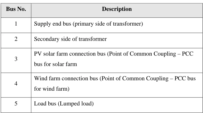
Table 2.1 Study system bus identification

Bus No. Description

1 Supply end bus (primary side of transformer)

2 Secondary side of transformer

3 PV solar farm connection bus (Point of Common Coupling – PCC bus for solar farm

4 Wind farm connection bus (Point of Common Coupling – PCC bus for wind farm)

(44)

22

2.3 Network and Load Model

2.3.1 Grid Model

For steady-state analysis in PSS/E, the grid is represented by a slack bus/infinite bus

capable of supplying the required power at specified bus voltage. The generator

considered at slack bus can supply the active power (including total system loss and load)

required by the distribution network or it can absorb the excess active power in case of

reverse power flow due to distributed generators. Also, such generators can supply or

consume reactive power at specified voltage as required by the feeder.

For electromagnetic transient simulation in PSCAD/EMTDC, the grid feeding the

distribution line is represented by a voltage source behind equivalent source impedance

as shown in Figure 2.2. The equivalent series impedance of the grid consists of series

resistance, RSRC and the series reactance, XSRC. The voltage behind the reactance, E, is

fixed whereas the terminal voltage VBus-i depends on the loading condition of the

distribution feeder.

Figure 2.2 Grid modeled as voltage source with equivalent impedance

2.3.2 Transformer Modeling

Electric power grid basically consists of generation, transmission and distribution

systems which normally exist at different voltage levels. In such power grids,

transformers are widely used to connect the systems at different voltage levels. The

(45)

parameters, which consist of series resistance and reactance, are used to represent the

copper loss and the leakage flux of the windings, respectively. The copper loss and the

leakage flux for both the primary and secondary windings depend on transformer loading.

The net flux that links the transformer windings and the iron loss (hysteresis loss and

eddy current loss) are fixed for a transformer with rated voltage and independent of the

transformer loading condition. Shunt parameters, namely shunt resistance and reactance

are used to represent such fixed loss and flux in the transformer. The shunt resistance and

reactance are very high and their effect in the system is neglected for complete system

analysis. Also, copper loss in the transformer windings is significantly low compared to

the network losses and hence a loss less transformer is used for the study system. In this

scenario, the transformer can be modeled as a reactance XTR in series with an ideal

transformer between two system buses i and j as shown in Figure 2.3. VBus-i and VBus-j

denote the voltage at buses i and j, respectively.

Figure 2.3 Transformer model - ideal transformer with series reactance

2.3.3 Line Modeling

Electrical parameters of a transmission line are based on size of conductors and their

geometrical configuration. An overhead transmission line is represented by series

parameters (series resistance, , and reactance, ) and shunt parameters (shunt

conductance, , and susceptance, ) as below.

Ω/ ……… 2.1

/ ……… 2.2

(46)

24

For the medium voltage overhead feeder, these distributed line parameters are

represented by lumped model both for steady-state and transient analyses. The series

parameters are represented by equivalent resistance, R and equivalent reactance, X. The

shunt conductance, G is negligible for the overhead lines and half of capacitive

susceptance (Y/2) is used to represent shunt parameters on each terminal of the line. The

resulting equivalent -model, as shown in Figure 2.4, is used to represent the line

sections of the study system between Bus-i and Bus-j.

∙ ……… 2.3

∙ ……… 2.4

∙ ……… 2.5

,

Figure 2.4 Equivalent -model of overhead line (lumped parameters)

2.3.4 Load Model

The load in a distribution network consists of various types of heating, lighting and motor

loads. Individual loads vary widely in their performance characteristic. The equivalent

characteristic of the load viewed from the medium voltage side (secondary of the feeder

transformer) will be obtained by the net effect of the individual loads. The net active

power and reactive power of a given load are affected by the terminal voltage and the

(47)

Based on the study requirements, load models are broadly classified into two types: static

load models and dynamic load models. Static load models used in load flow studies are

expressed as steady state active and reactive powers as function of bus voltage and

system frequency. Dynamic load models, on the other hand, are used for stability studies

that involve load dynamics (as in voltage stability studies). Static load models are

traditionally classified into following three types [41].

 Constant power load model (Constant P): A static load model in which the

power does not vary with voltage magnitude. It is also referred to as

constant MVA load model.

 Constant current load model (Constant I): A static load model in which the

power varies directly with voltage magnitude.

 Constant impedance load model (Constant Z): A static load model in which

the power varies with the square of the voltage magnitude.

Though the individual characteristics vary widely, the aggregated load characteristic of

typical commercial and domestic loads are given as:

1 . ……… 2.6

1 . ……… 2.7

,

(48)

26

In this thesis constant power static load models are used for load flow studies as well as

transient (fault) studies. The load is considered to be lumped at the receiving end (Bus 5)

of the network. The constant power load with power factor of 0.91 lagging is considered

both for steady state and transient studies.

2.4 PV System Model

PV solar system basically consists of photovoltaic cells that produce DC electricity, an

inverter that converts DC to AC, an LC line filter that removes the harmonic components

produced by inverter, and coupling transformer that connects AC side of the PV system

to the point of common coupling (PCC) at grid. The DC side voltage, VDC, DC current,

IDC, AC side three phase voltages VABC and three phase line currents IABC are used as input

to the inverter controller which generates gate drive pulse signal to operate inverter

switches. A schematic diagram of PV system is shown in Figure 2.5.

Figure 2.5 PV Solar System

2.4.1 Photovoltaic Array

Photovoltaic cell, which consists of semiconductor material, is the basic unit of a PV

(49)

semiconductor PV cells are classified in three categories: Monocrystalline,

Polycrystalline, and Amorphous. Monocrystalline PV cells require pure silicon and

complicated crystal growth technology making them most expensive among various PV

cell technologies. However, these monocrystalline cells have highest efficiency and are

used in critical applications where generating more power utilizing less space is of

importance. Polycrystalline cells, on the other hand, contain many crystals and have a

less perfect surface than monocrystalline cells. Polycrystalline PV cells are widely used

due to their low cost and moderate efficiency. Amorphous cells, with the thinner silicon

wafers compared to crystallized PV cells, are more flexible than the other types. Though

the efficiency is least of the three, amorphous silicon cells have gained wider application

in recent days with the development of thin film photovoltaic (TFPV) technology. With

the this technology, low cost PV modules can be made in variety of sizes and shapes.

The basic units of photovoltaic technology referred as PV cells are connected in a

combination of series and parallel connection to increase the voltage and current

available from the photovoltaic cells. Such combination of cells is referred as PV solar

module. Typical solar module consists of 36 to 72 cells and ranges from 75 W to 350 W

in peak output power (Wp). A PV array is the combination of PV modules connected in

series and parallel to match the requirement of inverter for grid integration. A PV solar

farm may consist of a number of solar arrays based on its capacity.

(50)

28

A solar module can be represented by simplified equivalent circuit as shown in Figure

2.6. Based on this equivalent circuit, the relationship between the terminal voltage of

solar module and the current delivered to the load is:

∙

1 ∙ ……… 2.8

,

/

1.381 10 /

°

Based on the equivalent circuit shown in Figure 2.6 and relationship given in (2.8), a

typical I-V characteristic curve for given insolation and cell temperatures at standard test

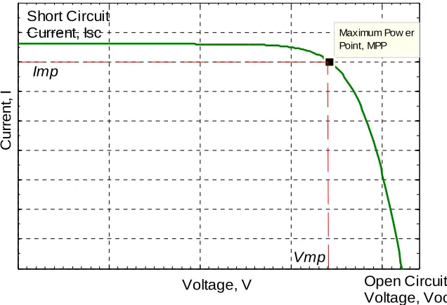
condition is depicted in Figure 2.7. The voltage at open terminals of the module is

referred as open circuit voltage (VOC). For this open circuit case, the voltage across the

terminals is maximum for given operating conditions and the current through the PV

terminals is zero. The terminal voltage decreases slightly as the current drawn from the

PV terminals increases. This drop in voltage is affected by the series resistance value RSE

(51)

current increases beyond certain value. This sharp fall in current depends on the value of

shunt resistance RSH of the module (∆ / . The maximum current from the PV

module, when its terminals are shorted, is referred as short circuit current, ISH.

This unique I-V characteristic of PV modules provides self-regulation for battery

charging applications. However, an additional control is provided to operate PV modules

for maximum power output when connected to the power grid. The nominal voltage and

current magnitude are identified by the voltage and current at maximum power point at

the nominal insolation and nominal ambient temperature (standard test conditions). The

short-circuit current and open-circuit voltage are slightly higher than respective nominal

voltage and current. The ratio of the maximum power . to the product of

open-circuit voltage and short-open-circuit current . ) as given in (2.9) is defined as the fill

factor of PV module

Figure 2.7 A typical current-voltage characteristic of PV module

∙

∙ ……… 2.9

,

Maximum Pow er Point, MPP

Voltage, V

C

u

rr

e

n

t, I

Short Circuit Current, Isc

Open Circuit Voltage, Voc

(52)

30

Fill factor generally varies between 0.8 and 0.9. It depends on series and shunt resistance

values shown in the equivalent circuit of Figure 2.6. Fill factor represents the measure of

efficiency of the PV module. For nominal operating condition, the variation in terminal

voltage with the variation of power output is minimal. Accordingly, the DC side voltage

of the solar inverter can be approximated by the nominal DC voltage to study the impact

of PV solar farm integration to the grid. Such equivalent DC voltage source along with

series resistance to represent the DC side loss, are used to model the PV solar array. The

MPPT is not modeled in the PV solar farm model in this thesis, as only the inverter

capacity remaining after real power generation is being utilized for voltage control.

2.4.2 Line Filter

Voltage Source Converter (VSC) based PV inverters produce various harmonic

components based on the control strategy and switching frequency [48]. The pulse width

modulation (PWM) technique can be used to eliminate lower order harmonics and reduce

the total harmonic distortion due to converters.. In sinusoidal pulse width modulation

(SPWM), which is the most common PWM technique, the magnitude and frequency of

the sinusoidal fundamental component are controlled by pulse width modulation. In such

converters, the higher the switching frequency, the better is the quality of the resulting

waveform and smaller the filter capacitor and inductors requirements.

A low-pass LC filter, as shown in Figure 2.8, is used to remove the harmonic components

and provide smooth sinusoidal waveform at the point of common coupling (PCC). In

PWM technique, the information about the fundamental component of the output voltage

is embedded (modulated) in the widths of the output voltage pulses. The demodulation

takes place in the output low-pass filter (LC filters), where the switching harmonics are

separated from the fundamental component, or in the inductive load, where the pulsed

(53)

; . .

The odd value of frequency modulation index is chosen as it provides a half-wave

symmetry in resulting output waveform. Half-wave symmetry is useful in converter

output as it eliminates even harmonic components. The harmonic components in output

waveform will appear as sidebands around the switching frequency and its multiples. The

frequencies of harmonic components are given by the following expression.

∙ ∙ ……… 2.10

Here value of k is even when j is odd, and k is odd when j is even. The frequency

modulation is selected in such a way that significantly higher order harmonics will appear

in the output (which are relatively easier to filter out) and switching loss is maintained

within acceptable value.

The series inductor (Lf ) used in the LC filter provides sufficient impedance between the

AC side of the inverter and the point of common coupling of the grid. The shunt

capacitor (Cf ) provides attenuation to the harmonic components of the inverter AC side

voltage.

Novel Control of PV Solar and Wind Farm Inverters as STATCOM for Increasing Connectivity of Distributed Generators

Scholarship@Western

Scholarship@Western

Novel Control of PV Solar and Wind Farm Inverters as STATCOM

Novel Control of PV Solar and Wind Farm Inverters as STATCOM

for Increasing Connectivity of Distributed Generators

for Increasing Connectivity of Distributed Generators

ABSTRACT

ACKNOWLEDGMENTS

TABLE OF CONTENTS

LIST OF TABLES

LIST OF FIGURES

LIST OF ABBREVIATIONS

LIST OF SYMBOLS

Chapter 1

1

INTRODUCTION

1.1 Growth of Wind Power and PV Solar Power Based

Distributed Generators

1.2 Issues with Grid Integration of DGs

1.2.1

Steady state voltages

1.2.2 Temporary

overvoltage

1.3 Conventional Mitigation Measures for Voltage Issues

1.3.1 Voltage

Regulation

1.3.2 Reactive

Power

Compensation

1.4 FACTS Controller based Mitigation Measures for

Voltage Issues

1.4.1

Static Synchronous Compensators (STATCOM)

1.4.1.1 Principle

of

Operation

1.4.1.2 STATCOM

Controller

1.5 Mitigation Measures using DG based STATCOM

1.5.1

PV Solar Farm based STATCOM (PV-STATCOM)

1.5.2

Wind Farm based STATCOM (Wind-STATCOM)

1.6 Motivation

of

Thesis

1.7 Scope of Research

1.8 Objective of the Thesis

1.9 Outline

of

Thesis

Chapter 2

2

SYSTEM MODELING

2.1 Introduction

2.2 Study

System

2.3 Network and Load Model

2.3.1 Grid Model

2.3.2 Transformer Modeling

2.3.3 Line Modeling

2.3.4 Load Model

2.4 PV System Model

2.4.1 Photovoltaic Array

2.4.2 Line Filter