Structural Fragility of Piping Systems using Equivalent Elastic Time-history Simulations under Bayesian Framework

Structural Fragility of Piping Systems using Equivalent Elastic Time-history

Simulations under Bayesian Framework

Sashi Tadinada1, Shinyoung Kwag2, 3, and Abhinav Gupta4 1

Senior Research Scientist, AIG, US

2

PhD Student & Research Assistant, CNEFS, North Carolina State University, US

3_{Senior Researcher, Korea Atomic Energy Research Institute, ROK} 4

Associate Professor & Director, CNEFS, North Carolina State University, US

ABSTRACT

The main objective of this study is to effectively evaluate seismic fragility of nonlinear inelastic connections in a piping system using linear elastic time-history analyses and Bayesian inference. Typical piping systems are characterized to have (a) essentially linear elastic stress-strain behavior; (b) damage due to excessive inelastic deformation at specialized nonlinear inelastic locations such as T-joint connections, elbows, valves, etc.; (c) low ductility (<3.0) corresponding to failure. Since the system is largely linear elastic, we utilize the equivalent linearization method (ELM) to describe the localized inelastic nonlinearities. The reason to use this is that one of the critical limitations in the seismic fragility analyses of structures under probabilistic simulation framework is the enormous computational costs associated with real structures described by intensive nonlinear inelastic Finite Element (FE) models.

The ELM in seismic fragility analyses must seek to minimize the error between the maximum responses which indicate the damage. For this, we introduce a concept called equivalent elastic limit state (ELS) into seismic fragility analyses. By studying a large number of representative structural systems which are essentially linear elastic but characterized by localized fragile inelastic nonlinearities, we propose a model to compute seismic fragility curves using only linear elastic time-history simulations. It is revealed that the seismic fragility using the model and linear elastic time-history simulation is quite close to the actual fragility, and the fragility using this approach can be successfully incorporated with Bayesian inference to obtain more accurate result. The efficacy of the approach is finally confirmed in an example of a full-scale piping system with fragile T-joint connections.

INTRODUCTION

Within the seismic probabilistic risk assessment (SPRA) framework, the reliability of structures, systems and components (SSCs) is described as seismic fragility (or seismic vulnerability). From a simulation perspective, multiple nonlinear inelastic (called as nonlinear in this study) time-history analyses are required for the seismic fragility analysis of the structural systems. It is attributed to the fact that the systems usually undergo the nonlinear behavior under large seismicity.

Specifically, the large-scale piping systems have three distinct properties from the observation in most of the experimental fragility studies: (1) the system is predominantly linear elastic (called as linear in this study) which means a substantial proportion of the total system has deformations below the yield limits; (2) the risk of damage is typically due to excessive deformations at the localized nonlinear joint connections; (3) the damage limit states like “First Leak” etc. tend to occur at low levels of ductility (2.0

~ 3.0). This means that piping systems can be modeled as essentially linear structures with fragile connections that exhibit localized nonlinear behavior. Since the system is largely linear, we can utilize the equivalent linearization method (ELM) to describe the localized nonlinearities to reduce computational cost.

linear time-history analyses, and Bayesian inference. For this, ELS concept and ELS V*equation for general piping model coupled with localized fragile nonlinear element is proposed by simulating a large number of simplified coupled structural systems. This is because the ELM in seismic fragility analyses must seek to minimize the error between the maximum responses which indicate the damage. Within the technique, the prior fragility curve is obtained by using ELS V* and linear time-history analyses. Then, the prior fragility curve is updated with a few number of nonlinear time-history results in the Bayesian inference. The efficacy of the approach is finally confirmed in a real example of a full-scale piping system with fragile T-joint connections in a hospital.

BAYESIAN UPDATING IN SEISMIC FRAGILITY

The seismic fragility is represented as a conditional probability of failure or collapse of SSCs to exceed specified failure limit state G(.) at a given seismic intensity parameter a. These seismic fragility and limit state can be mathematically expressed in Equation 1 and Equation 2:

( )

(

( )

)

f

P a =P G < a (1)

G= -C D (2)

where Pf(a) is the probability of failure given a seismic parameter a; a is typically represented as peak

ground acceleration (PGA), spectral acceleration (SA), peak ground velocity (PGV) or moment magnitude (Mw); C denotes the capacity of the SSC corresponding to the failure limit state; D represents response

demand on the SSC at a given seismic intensity parameter.

In a current stage, the seismic fragility curve within a SPRA framework is usually assumed to follow log-normal cumulative distribution function (CDF) determined from two parameters (Kennedy et al. 1980). Two specific parameters of the log-normal CDF can be obtained by fitting them to the empirical, experimental and simulation data which are available. The log-normal fragility curve is expressed in Equation 3:

(

)

( )

( )

f

R

a c

P a

b

é + ù

= F ê ú

ë û

θ ₍₃₎

where Φ[∙] is the standard Gaussian CDF; c is the median seismic capacity having a log-standard deviation βU of uncertainty in our knowledge; Φ-1(∙) is the inverse of the standard Gaussian CDF; βR is a

log-standard deviation of inherent randomness having some degree of uncertainties; θ _{(= [cβR] ) is two}

parameters of fragility curve.

In real situation, the seismic fragility curve obtained from Equation 3 will be changed by the newly observed empirical, experimental, or more precise simulation data. Bayesian updating strategy can bring the additional data d into the current fragility model for more accurately predicting seismic fragility curve. In this method, current (so called prior) seismic fragility curve Pfprior

(

)

into future (so called posterior) seismic fragility curve P_fpost

(

)

(

)

(

) (

)

post prior

f f

P a d =

ò

(

)

(

) ( )

(

) ( )

|

f f

f

f f d

=

ò

d θ θ

θ d

(

)

(

(

)

)

(

(

)

)

1

| ; i 1 ; i i

k _{r n r}

i prior prior

f i f i

i i

n

f P a P a

r -= æ ö = _{ç ÷} -è ø

Õ

d θ θ θ ₍₆₎

where f (θ_{|d) is the posterior joint probability density function (PDF), f (d|}θ_{) is the likelihood function,}

and f (θ_{) is the prior joint PDF of two parameters of the lognormal fragility model. d is the k}th _{number of}

data as formatted in d = [ [a1 …ai … ak]T [n1 …ni… nk]T [r1 …ri … rk]T ] with number of observed failure ri

out of total number of structural specimens ni at a given intensity parameter = ai, and Π is the product of

all k of a = ai levels. This study uses Metropolis-Hastings algorithm (Metropolis et al., 1953; Hastings,

1970) of Markov Chain Monte Carlo (MCMC) for the integration of equation 4 and PGA for a.

EQUIVALENT ELASTIC LIMIT STATE (ELS) CONCEPT

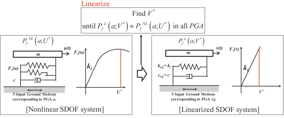
The equivalent elastic limit state (ELS) is the optimal displacement value V* as a failure limit state for the linearized system which makes the seismic fragility evaluated from linearized system close to the seismic fragility of the nonlinear system. The linearization for the nonlinear system is conducted by using same initial stiffness and damping coefficient of nonlinear system, but adopting the different ELS V* which is not same as the nonlinear limit state U*. The conceptual ELS idea in a single degree of freedom (SDOF) system is illustrated in Figure 1. The ELS V* can be obtained by solving optimization problem in Equation 7 where failure probabilities from the linear system responses Pf L in Equation 8 are close to

failure probabilities of nonlinear system Pf NL in Equation 9. The objective function is represented as the

root squared error between Pf L and Pf NL:

{ }

( )

(

(

)

(

)

)

2 *

Find *

1

1

Minimize ; ;

k

NL L

f i f i

V V

i

f V P a U P a V

k

= =

å

(

)

( )

(

( )

)

1

; | 1 1 /

N

L i

f

i

P a V P v a V PGA a a v g V N

=

= é_ë > = ù »_û

å

(

)

( )

(

( )

)

max max

1

; | 1 /

N

NL i

f

i

P a U P u a U PGA a u a U N

=

é ù

= _ë > = _û»

å

where k is the number of PGA levels; N is the number of time-history analyses at one level of PGA; and

vmax (a) and umax (a) denote the random variables representing the peak displacement response under an

(

)

(

)

*

* *

Find

until _fL ; _fNL ; in all

V

P a V »P a U PGA

Fs(u)

U*

(

)

;

NL f

P a U

[Nonlinear SDOF system]

m

Fs(u)

c

NInput Ground Motions corresponding to PGA ai

k

(

)

; L f

P a V

m

keq= ki

ceq= c

NInput Ground Motions corresponding to PGA 1g

v(t)

V*

Fs(v)

[Linearized SDOF system]

k

u(t)

Linearize

Figure 1. ELS concept

ELS MODEL DEVELOPMENT FOR SIMPLIFIED COUPLED STRUCTURAL SYSTEM

In order to generalize ELS of the piping system having the localized fragile nonlinear element, the sensitivity of ELS of the nonlinear element of the piping system should need to be studied since the responses of the nonlinear element of the piping system are much affected by the tuning ratio between the natural frequencies of the main piping system and nonlinear element. The simplified coupled structural system such as 2-DOF system is considered as shown in Figure 2. As shown in Figure 2, main piping system is represented as linear SDOF model and localized fragile nonlinear element is expressed as bi-linear SDOF model. Here, mp and ms are masses, ξp and ξs are damping ratios, kp and ks are initial stiffness, α is post-yield stiffness ratio of ks, Δy is yield displacement, U* is limit state of nonlinear model, μ is

displacement ductility capacity, and fs and fp are natural frequencies regarding initial stiffness. The tuning

ratio ηis defined in Equation 10.

p s

p s

f f

f f

h=

-+ (10)

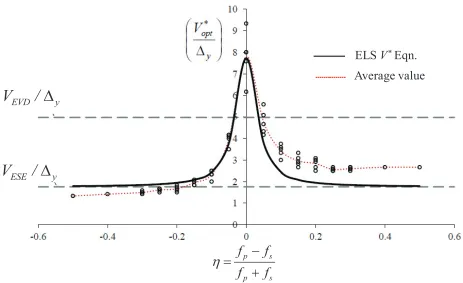
For getting ELS relationship in a change of tuning ratio, 70 different systems with various combinations of natural frequencies (fp and fs) are selected at the specified displacement ductility capacity.

The systems are assumed to be classically damped having damping ratio 0.05 at all modes. The mass ratio

γ (=ms/mp) and the post-yield stiffness ratio α in bi-linear curve is 0.001 and 0.1, respectively. The

displacement ductility capacities μ are considered at 2 and 3. The 12 (=k) PGA levels are chosen between 0.25g and 3.0g at an interval of 0.25g. The 75 (=N) earthquake ground motions are picked out (Gupta & Choi, 2005). Using equation 7, the V*opt for 70 different systems at μ = 2 and μ = 3 are obtained and

represented in Figure 3 and Figure 4.

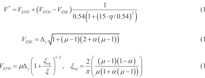
linearization methods are not handled in a detailed manner. The final general equation ELS V* fitted into numerical simulation data by using Cauchy probability density function and two equivalent linearization methods is represented as followings:

(

)

(

)

(

)

*

2

1

0.54 1 15 / 0.54

EVD EVD ESE

V V V V

h

= +

-+ × (11)

(

)

(

(

)

)

1 1 2 1

ESE y

V = D + m- +a m- (12)

(

)(

)

(

)

(

)

1/ 2

1 1 2

1 ,

1 1

eq

EVD y eq

V m x x m a

x p m a m

æ - - ö

æ ö

= D _ç + _÷ = ç_ç ÷_÷

+

-è ø _{è ø} (13)

The Figure 3 and Figure 4 also illustrate the numerical simulation data above and ELS V* of Equation 11 in tuning ratio and V*/Δy domain.

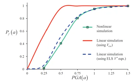
Finally, for confirming the efficiency and validity of this Equation 11, the example of nearly tuned coupled structure having mp = 32,200 kg, ms = 32.2 kg, kp = 1e7 N/m, ks = 12,216 N/m, α = 0.1, Δy =

0.06 m and μ = 2 is studied. Figure 5 shows predicted fragility curve predicted from 900 (=12x75) nonlinear analyses and 75 (=1x75) linear analyses using ELS V* equation for this example structure. It can be seen that the seismic fragility curve using 75 linear analyses based on ELS V* equation is quite close to that using 900 nonlinear analyses. From this result, it is confirmed that we can significantly reduce the computational time by using ELS concept when getting seismic fragility curve even though not sacrificing the accuracy.

m

k

F

(

x

)

m

Input ground motion

f

f

k

α

_k

F

(

x

)

Δ

U

[Bi-linear model]

[Simplified 2-DOF piping system]

p

x

s

x

y

D

*

y

U

= ×D

m

ESE y

V

/

D

EVD y

V

/

D

p s

p s

f

f

f

f

h

=

-+

Average value

ELS

V

_Eqn.

Figure 3. ELS V* representations of 70 systems at μ=2

ESE y

V

/

D

EVD y

V

/

D

p s

p s

f

f

f

f

h

=

-+

Average value ELS V*_Eqn.

Nonlinear simulation

Linear simulation (using V_ese)

Linear simulation

(using ELS

V

_eqn.)

( )

P a

( )

PGA a

Figure 5. Seismic fragility curves from nonlinear analyses and linear analysis using ELS V* equation for the example structure

APPLICATION: HOSPITAL PIPING SYSTEM FRAGILITY

In this section, the ELS concept and Bayesian updating strategy for efficiently determining the seismic fragility curve for the piping system having the localized nonlinear element is illustrated by using the 2-inch water-sprinkler system in hospital having threaded T-joint connection as shown in Figure 6. The prior seismic fragility curve is calculated by using ELS V* equation and linear time-history analyses. This prior fragility curve is updated by Equation 4 and a few number of additional nonlinear time-history analyses. The detailed information and comprehensive fragility analyses of this piping system using nonlinear time-history simulations were represented by Ju et al. (2011) and Ju (2012). The fundamental frequency of overall piping system is fp = 1.82 Hz and the natural frequency of the threaded T-joint

connection assembly is fs = 60 Hz. The yield curvature θy (=Δy) is 0.0063 rad. The limit state of T-joint

connection is U* = 0.022 rad. Therefore, η = (1.82-60)/(1.82+60) = -0.94 and μ = 0.022/0.0063=3.49. The 75 ground motions above mentioned and 6 different PGA levels ([1g, 1.2g, 1.5g, 2.0g, 2.5g, 3.0g]) are used in this application

In a first step, for creating prior seismic fragility curve, the ELS V* and 75 linear analyses at 1g PGA level are performed. The ELS V* is computed as 0.159 rad. Based on this ELS V*, the prior seismic fragility curve is obtained by Equation 8 and 75 linear time-history analysis results. In a second step, using the prior information in conjunction with the lognormal fragility model of Equation 3, we define the following prior distributions for the random parameters c ~ log N (cm= 2.009g, βU = 0.24) and βR ~ N

(0.4097,0.2) representing median capacity and log-standard deviation. Total 90 Nonlinear time-history analyses are performed at 6 different PGA levels and the prior fragility curve are updated using Equation 4. The results are illustrated in Figure 7 with the actual fragility curve based on 360 nonlinear analysis results.

curve with 360 nonlinear analyses. This feature can help us efficiently conduct fragility analysis even with limited amount of simulation data.

Figure 6. Hospital main piping system with a 2-inch branch containing the threaded T-joint

Actual curve using 360 nonlinear simulation data

Curve using prior curve & Bayesian updating w/ 90 nonlinear simulation Prior curve using ELS V*_{and 75}

linear simulation data

Nonlinear simulation data

CONCLUSION

In this paper, the effective technique for getting seismic fragility of nonlinear connections in a piping system using linear time-history analyses and Bayesian inference was proposed. For this, ELS concept was introduced, and ELS V* equation for general piping model coupled with localized fragile nonlinear element was proposed by simulating 70 simplified coupled systems. Within the technique, the prior fragility curve was obtained by using ELS V* and linear analyses. Then, the prior fragility curve was updated with a few number of nonlinear time-history results in the Bayesian inference framework.

It was demonstrated through the real-life example of a hospital main piping system (2" water-sprinkler branch with a fragile threaded tee-joint) that the technique based on prior estimates using equivalent linear elastic analyses in conjunction with Bayesian updating by incorporating nonlinear simulation data was an effective approach to minimize the total computational effort of evaluating seismic fragility of critical nonlinear connections in the large piping system.

ACKNOWLEDGEMENTS

The authors sincerely wish to thank the financial support of Center for Nuclear Energy Facilities and Structures (CNEFS), and Civil, Construction and Environmental Engineering (CCEE) Department of North Carolina State University (NCSU) for the writing of this publication.

REFERENCES

Jacobsen L.S. (1930). “Steady Forced Vibrations as Influenced by Damping.” ASME Transactions, 52(1), 169-181.

Ju, B., Tadinada, S.K. and Gupta, A. (2011). “Fragility Analysis of Threaded T-joint connections in

Hospital Piping Systems,” Proc., ASME Pressure Vessels and Piping (PVP) Conference, Baltimore. Ju, B. (2012), Seismic Fragility of Piping System, PhD thesis, North Carolina State University, Raleigh,

NC, USA.

Kennedy R.P., Cornell C.A., Campbell R.D., Kaplan, S., Perla H.F. (1980). “Probabilistic seismic safety of an existing nuclear power plant,” Nuclear Engineering and Design, 59, 315–338.

Veletsos, A.S. and Newmark, N.M., “Effects of inelastic behavior on the response of simple systems to

earthquake ground motions,” Proceedings of the 2nd World Conference on Earthquake