Analysis of DNA diversity by spatial autocorrelation.

(1)

Analysis

of

DNA Diversity

by

Spatial Autocomelation

Giorgio Bertorelle*

and

Guido Barbujanit

*Dipartimento di Biologia, Universita di Padova, 35121 Padova, Italy and tDipartimento di Scienze Statistiche, Universita di Bologna, 40126 Bologna, Italy

Manuscript received November 21, 1994

Accepted for publication February 25, 1995

ABSTRACT

Two statistics are proposed for summarizing spatial patterns of DNA diversity. These autocorrelation indices for DNA analysis, or AIDAs, can be applied to RFLP and sequence data; the resulting set of autocorrelation coefficients, or cowelogram, measures whether, and to what extent, individual DNA sequences or haplotypes resemble the haplotypes sampled at arbitrarily chosen spatial distances. Analyses

of computer-generated sets of data, and of RFLP data from two natural populations, show that AIDAs allow one to objectively and simply identify basic patterns in the spatial distribution of haplotypes. These statistics, therefore, seem to be a useful tool both to explore the genetic structure of a population and to suggest hypotheses on the evolutionary processes that shaped the observed patterns.

P

OPULATIONS are said to show genetic structure whenever the distributions of their genes do not conform to panmictic expectations. Evolutionary processes may be inferred from data on the genetic structure of populations. Ideally, such inferences require two phases. Patterns of genetic variation are initially summa- rized by descriptive statistics, and then they are interpre- ted by comparison with the patterns predicted by theoretical models. The second phase includes the estimation of parameters quantifylng the effects of mutation, selection, inbreeding, drift, or gene flow.

Well-established methods allow the analysis of population structure at the level of classical protein markers (see e.g., WIJSMAN and CAVALLI-SFORZA 1984). Although a regular, clock-like rate of allele frequency divergence is sometimes assumed (CAVALLI-SFORZA et al. 1988; BAR-

W T E S et al. 1990), the emphasis in most such studies has been on factors such as adaptation to variable habi- tats, patterns of gene flow, and isolation by distance. In other words, the genetic population structure is often analyzed with an eye to its geographical, rather than historical, determinants.

In contrast, for DNA data, the analysis generally leads to reconstruction of genealogies of alleles (reviewed in HUDSON 1990). In this way, under neutrality assump tions, the focus shifts to processes occurring in the course of the populations’ history, typically branching events. There are, however, problems.

As

FELSENSTEIN (1982) first remarked, history and geography jointly determine patterns and levels of genetic diversity; in the absence of nongenetic information, their effects are difficult to disentangle. Equal levels of haplotype diversity, for example, may be caused by a stable regime

Cmrespondingauthur: Guido Barbujani, Dipartimento di Scienze Sta- tistiche, UniversitA di Bologna, via Belle Arti 41, 40126 Bologna, Italy. E-mail: [email protected]

Genetics 140: 811-819 (June, 1995)

of gene flow constrained by geography or by episodes punctuating the population’s history, such as the colonization of a new habitat (see e.g., TEMPLETON 1993).

Several attempts are being made to tackle this prob- lem, by incorporating a geographic perspective into methods for the study of DNA variation. SLATKIN (1989, 1991) and SLATKIN and MADDISON (1989,1990) worked out how to estimate the minimum numbers of migration events from gene genealogies, looked for empirical relationships linking such parameters with gene flow rates ( m ) , inbreeding coefficients and effective population sizes ( N e ) , and extended their approach to non- equilibrium situations (SLATKIN 1993). EXCOFFIER et al. (1992) developed a method for the analysis of molecular variance, AMOVA. They proposed new statistics re- sembling WRIGHT’S (1965) F, whose values depend on the correlations between haplotypes at various levels of subdivision, i.e., within demes, between demes within regions, among regions, etc. TEMPLETON (1993) proposed to analyze evolutionary trees by a cladistic procedure (TEMPLETON et al. 1987) designed to identify, respectively, areas of population expansion, and areas where gene flow has been restricted.

In this paper, we present two indices of spatial autocorrelation, specifically developed for treatment of molecular data. In classical spatial autocorrelation analysis (SOW and ODEN 1978a,b), levels of genetic resem- blance are calculated between pairs of localities, within arbitrary distance classes. Spatial patterns of allele frequencies are thus represented by sets of coefficients (MOWN’S

I

or GEARY’S c) calculated at different distances, or cowelograms.

Correlograms give an easy-to-understand depiction of spatial patterns of variation. They can be compared across different geographical regions and genetic markers, thus suggesting obvious neutrality tests (SOUL et

(2)

812 G . Bertorelle and G. Barbujani

andJACQUEz 1991).

fb

they are, spatial autocorrelation methods can be applied to DNA data if the data are transformed in such a way as to be treated as allele frequencies (see COSTA et al. 1992). This transforma- tion, however, is possible only if several sequencies are sampled in each population, and it implies a loss of information because the haplotypes are classified as being the same or different, and the amount of sequence differences between them is not considered.

Ideally, an autocorrelation index for DNA analysis (we propose to call it AIDA) should measure whether, and to what extent, individual DNA sequences (or haplotypes) resemble the sequences sampled at different localities. In this way, this index could be employed for exploratory data analysis (SLATKIN and ARTER 1991). Few sequences sampled in different localities can be used to objectively recognize nonrandom distributions of haplotypes. Correlograms inspection may also help in testing hypotheses on the evolutionary history of the populations under study.

The two autocorrelation indices, or AIDAs, described in this paper, are a product-moment coefficient, analo- gous to MORAN’S

I,

and a distance-like coefficient, analo- gous to GEARY’S c (SOKAL and ODEN 1978a). Both are based on comparisons between individual sequences, rather than between frequencies of alleles or haplotypes. Because in this way genetic relatedness is inferred from sequence similarity, only parts of the genome should be considered that either are haploid or can be treated as such (e.g., DNA segments where recombination can safely be ruled out). Indeed, a single crossing- over may result in large sequence differences between haplotypes. Under recombination, therefore, sequence differences are no longer a measure of evolutionary distance, and this may bias the inferences drawn from autocorrelation analysis. However, we shall also show how some sets of data where recombination has oc-

curred may be liable to spatial autocorrelation analysis. A matrix is then calculated, of phenetic (namely counts of sequence differences between haplotypes) or evolutionary distances (estimates of the number of evolutionary events, mutation and possibly recombination, separating pairs of haplotypes); from either matrix is the correlogram evaluated.

REPRESENTATION OF DATA

Suppose there are S segregating or polymorphic sites in a DNA fragment, studied either by DNA sequencing or by restriction site analysis. In general, we shall assume that recombination is absent, and that only two different nucleotides can occur at each polymorphic site. The latter is a widely used assumption (see e.g., KREIT- MAN 1983; EXCOFFIER et al. 1992; EXCOFFIER and

SMOUSE 1994), consistent with the infinite-site model

(KIMURA 1969; WATTERSON 1975), but not necessarily implying it. Following EXCOFFIER et al. (1992), an indi-

vidual sequence, or haplotype, will be represented as a binary vector

p =

[PI,

p z , p 3 ,

. . .

, P S I . (1)

In the case of DNA sequence data,

p,

represents either of the possible nucleotides at each of the S sites, arbitrarily labelled as 0 or 1. Alternatively, for RFLP data,

p ,

represents the presence or absence of one of S possible restriction sites.

A modification is necessary when more than two different nucleotides occur at the same site. Os and 1s will then indicate presence or absence of one specific nucleotide at a certain site. For example, A, C, G, and T may be coded as 1000,0100,0010, and 0001, respectively. In this way, each segregating site will be represented by a four-digit binary code. For the sake of simplicity, however, we shall refer to the simpler case of two alternative nucleotides.

Binary digits can also be used to represent presence and absence of a repeat in a microsatellite; however, the autocorrelation analysis of these data is complicated by the fact that recombination is probably a major force generating VNTR diversity (see WING 1993).

Representing haplotypes by binary vectors corre- sponds to the approach labelled as phenetic by EXCOF-

FIER et al. (1992). An alternative, evolutionary, approach exists; it will lead to different results if homoplasy is high. For the evolutionary approach, a minimum-span- ning tree (PRIM 1957; ROHLF 1970) is constructed; the 1s in the p vector will then represent the occurrence of a mutational event along the branches of the tree that separate the sequence identified as ancestral (coded by a string of Os) and the sequence of interest. Errors in the definition of the ancestral haplotype do not modify the results of the analysis, because they do not affect the number of mutational steps separating any pairs of haplotypes. Here we note that recombination, deletion and duplication events may sometimes be placed in the tree with a certain degree of confidence (see e.g., COSTA et al. 1991). In this case, and only in this case, can AID& be employed to summarize geographic diversity even for DNA regions affected by recombination. Of course, only for the analysis of haploid DNA is there a one-to-one correspondence between individuals and haplotypes. Under both the phenetic and the evolutionary approach, each haplotype in the study will be represented by the spatial coordinates of its place of origin or sampling, and by its p vector.

CALCULATION OF AIDAS

(3)

Spatial Patterns Variation

dence limits by a randomization procedure; and (6) significance testing.

Steps 1 and

2

deal with geographical information. They are straightforward and do not differ from the initial steps of classical autocorrelation analysis. A matrix of painvise spatial distances between individuals is calculated, and arbitrary distance class boundaries are defined. Popular criteria for defining class boundaries are equal intervals (i.e., point pairs are allocated to classes of equal width) and equal frequencies (i.e., class limits are defined in such a way that equal numbers of point pairs fall in each class) (WARTENBERG 1989). Alternatively, specific class boundaries may be chosen. For each of these classes, however defined, an AIDA will be computed.

In step 3 one turns to molecular data. For each of the Ssites, an average is calculated across all individuals. Such averages will be >O and <1, because the mono- morphic sites are excluded. The average vector is a mathematical artifact that does not represent any biological reality. The values of its individual components are simply the frequencies of either of the alternative nucleotides at each site (under the phenetic criterion), or the frequency at which each specific evolutionary change (each mutation event or, when possible, each deletion, duplication or recombination) is observed in the sample (under the evolutionary criterion).

For each class defined in step 2, the following AIDAs, respectively called ZZand cc, by analogy with MORAN’S

Z

and GEARY’S c are thus calculated (step 4): n-1 R S

and

i = l k = l

n-1 n S

cc = k = l i = l J > i _n _S

9 (3)

i = l h = l

where n is the sample size, Wis the number of pairwise comparisons in the distance class of interest,

p,

and p j k are the haplotypes (i.e., the p values) of the ith and @

individuals, respectively, at the kth site, F k is the kth element of the average vector, and the weights wij are 1 if individuals i and jfall in the distance class of interest, otherwise they are 0. Summation is over the S sites, and for all n individuals in the sample. It is easy to assign different weights to sequence differences if necessary, i.e., to attribute a different importance to transitions and transversions, to substitutions and deletions, or to synonymous and nonsynonymous changes. In Equation (3), note that the summation of the quantities

p,

-

is equal to the number of sites differing between haplotypes i and j under the phenetic approach,

whereas it is the number of evolutionary steps between haplotypes

i

and

j

under the evolutionary approach.

The AIDAs thus defined share the statistical properties of related MORAN’S Zand GEARY’S c (CLIFF and O m 1981; RPLEY 1981). For large samples, they are distributed in the range -1 5

ZZ

I 1 and 0 5 cc I m.

Their expected values, under a randomization hypothesis, are as follows:

E(ZZ) = E(Z) = - l / ( n - 1) (4)

and

E(cc) = E(c) = 1. ( 5 )

Similarity between haplotypes, or positive autocorrelation, is shown by positive

ZI

values and by cc values close to 0; haplotype dissimilarity, or negative autocorrelation, results in Nand cc values at the other extreme of the range.

Haplotype divergence is constrained by the geneal- ogy of the sample studied. Occurrence of different mutations in different lineages causes linkage disequilibrium (SLATKIN 1994), especially when recombination is scarce or absent. The different sites in a DNA region, therefore, do not vary independently, and the variances of ZZ and cc, necessary for step 5, cannot be estimated on the assumption of independence of the segregating sites. The simplest alternative is a randomization a p proach (MANLY 1991); a null distribution of ZZand cc

values is constructed, assuming that haplotypes are randomly distributed in the geographical space.

To this end, sequences are randomly assigned to the sampled localities, retaining for each locality the observed sample size, and AIDA’s are recalculated. This operation is repeated for Nl times, so that an empirical distribution of

ZZ

and cc values is obtained, under the assumption of random haplotype distribution. From such an empirical distribution, confidence limits are estimated for each distance class, and the probability can be evaluated that a certain level of autocorrelation, observed in a distance class, may occur under the null hypothesis of no spatial structuring (step 6). By increasing the value of N,, any desired level of significance can be tested. This procedure, very similar to that employed for assessing the significance of MANTEL’S tests of matrix correlation (MANTEL 1967; SMOUSE et al. 1986), may require large amounts of computation: a faster permutation scheme is therefore reccomended for large samples. In this case, confidence limits are calculated only once, sampling N2 random pairs of h a p lotypes regardless of their spatial location. As before, this operation is repeated Nl times to found the empirical distributions of

ZZ

and cc. The lower N,, the more conservative will the test result. We suggest to use a value of Nl equal to the lowest number of comparisons observed in the distance classes analyzed.

(4)

814 G. Bertorelle and G. Barbujani

reviewed by ODEN (1984), the Bonferroni test (SOU and ROHLF 1981) being the simplest, if not the most sensitive. On the contrary, no established procedure exists for comparison of pairs of significant correlograms, although approximate tests can be conceived. In particular, bootstrapping (EFRON 1982) could be appropriate, and has actually been employed for the analysis of data in space (see e.g., DIACONIS and EFRON 1983), including genetic data (CAVALLI-SFORZA et al. 1988; TEMPLETON 1993). However, a general consensus has not been reached yet on whether spatial correlograms meet the conditions necessary for application of jack- knife and bootstrapping (N. L. ODEN, personal commu- nication). Therefore, we prefer not to deal with this issue in the present paper. The PC program AIDA is available on request.

APPLICATION OF AIDA TO ARTIFICIALLY GENERATED PATTERNS

In this section, the statistic 11 is applied to a set of computer-generated data. At this stage, we are mainly interested in studying whether this statistic can objectively recognize a random distribution of haplotypes from a simple spatial pattern; we also want to evaluate the sensitivity of AIDA when increasing levels of noise are added to a nonrandom spatial pattern.

Spatial distributions of sequences (referred to as sur- faces) were generated by assigning to each node of a square 10 X 10 lattice a haploid individual, whose haplotype is represented by one p vector with nine polymorphic sites ( S = 9). The nodes of the lattice are thus the spatial locations of the 100 individuals considered. There would be no additional difficulties if two or more haplotypes were placed at the same location, but this did not happen in the simulations we are presenting. Ten different haplotypes were considered. They can be regarded

as the products of successive mutations in a nonrecom- bining fragment of DNA, with each site being allowed to undergo mutation only once. Note that, because recombination is not considered to occur, the relative position of the polymorphic sites on the DNA molecule is irrelevant for this type of analysis. Haplotypes were as-

signed to the individuals of the lattice according to one of the following models of spatial variation.

Random variation: Under this model, 100 individual haplotypes were extracted from a rectangular distribution of the 10 possible haplotypes, and randomly assigned to the nodes of the lattice.

Pure gradient: We define a gradient as a pattern where the highest levels of haplotype differentiation are between individuals at the extremes of the simulated range, and individuals at intermediate locations also have intermediate haplotypes. The easiest way to simulate this, was by constructing a surface where the frequency of ones (or zeros) in the p vector increases along one direction. In evolutionary terms, this may be

000000000000000000000000000

A

OOOOOOoOi 000000001 00000000i 000000011OOo000011000000011 00OOo0111ooo000111000000111 000001 11 1 000001 11 1 000001 11 1 000011111 000011111000011111 0001 11

001111 011111 111111

000001

11 0001111 11 0011111 11 0111111 11 1111111

11 wooooa

100011111 100111111 101111111 1 11111111

1 oooooooc

B

0000001 11 OOOOOI 11 I oooooi I I I

000111111000000011000000011 000000011 000000001000111111 001111111 000111111000000000 000011111000000111 111111111 000000011000011111 000001111 000001111011111111 001111111 000111111 000111111 000011111 000111111000011111 000011111

FIGURE 1.-Examples of spatial distributions of haplotypes (p vectors) in two 3 X 10 sections of the data matrices generated under different models of spatial variation. (A) Pure North-South gradient; (B) Modified gradient, neighborhood size d = 4.

regarded as an extreme consequence of adaptation to an environmental gradient or as a result of a series of founder effects

(as

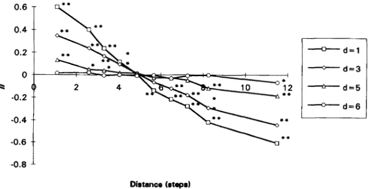
observed in experimental studies by EASTEAL 1988; U A C z et al. 1991; BOILEAU et al. 1992).

An example of such a distribution is in Figure 1A. Modified gradient: Under this model, a pure gradient was initially generated as described above; then it was modified by replacing the haplotype at each node with a neighbor, randomly chosen within a distance of dnodes of the lattice, d = 1 , 2 , 3 , 4 , 5 , 6 (d = 0 is the pure gradient). A modified gradient surface is represented in Figure 1B. Its evolutionary causes include the move- ment of individuals along a cline.

The distance classes for the correlograms were chosen following an equal-frequency criterion: each class included approximately the same number of painvise comparisons. Overall, 64 correlograms were calculated, describing respectively one purely clinal surface, and nine replicates each for the random surface and for the six modified gradients.

Results. The results of the analysis are given as median values of nine realizations of the same stochastic process, except for the pure gradient model, which was deterministic, and therefore was analyzed only once.

(5)

Spatial Patterns of DNA Variation

-0.8

I

Distance (steps)

FIGURE 2.-Correlograms describing a pure gradient and a random distribution of haplotypes. For the random distribution of haplotypes, the correlogram is the median of nine independent realizations of the same process. Ordinate, Zt abscissa, distance in steps, equal-frequency classes.

*

P

<

0.05;

**

P

<

0.01.

expectation. The median correlogram summarizing nine random distributions is reported in Figure 2.

The pure gradient resulted in a monotonic decrease of autocorrelation coefficients, from highly significant positive at short distances, to highly significant negative at large distances (Figure 2). This autocorrelation pro- file is identical to the one observed for clines of allele frequencies both in simulation and in field studies ( S o - KAL 1979; SOKAL et ul. 1989; S O W andJACQUEZ 1991). When gradients are disturbed by random noise (Fig- ure 3), the IIvalues are closer to 0, and the autocorrelation profiles are less steep, as expected (SLATKIN and

MARWAMA 1975). However, even for d = 5, autocorrelation in the extreme distance classes retains significance.

APPLICATION OF AIDA TO mtDNA DATA

The data:

As

an example of application of AIDA to natural populations, we consider two RFLP data sets,

0.4

o.6

1

\ * *

0.2

1

\.*

which show similar overall levels of genetic diversity and are both subdivided in several subpopulations, ar- ranged in a roughly linear manner along a transect.

The first data set comes from a study of the 2n = 60 chromosome species of the mole-rat (Spalux ehrenbergi)

in Israel. This is the second data set in the paper by NEVO et ul. (1993), and it includes eight populations. Based on the analysis of restriction fragments generated by 10 endonucleases in 69 individuals, 21 polymorphic sites and 15 different mtDNA haplotypes were described.

The second data set refers to

12

North-American populations of the “megarhyncha” group of the fox sparrow

(Passerella iliuca)

,

analysed by ZINK (1994) using 18 endonucleases; 14 different mtDNA haplotypes were ob-

served among 76 individuals, and 25 polymorphic sites were detected.

In both species, no haplotype was present in all the

0

a

-0.2

-0.4

-0.6

-d=l

-

d - 3

-

d - 5

Y,

* *

za

I

-0.8

1

Di8tanCe (8tW8)

(6)

816

0.5

0.4

0.3

0.2

0.1

a 0

-0.1

-0.2

-0.3

-0.4

G. Bertorelle and G. Barbujani

Mole-rat

T

140 160

-0.5

1

Distance (krn)

FIGURE 4.-Correlogram for the mtDNA data (NEVO et al. 1993) of the 2n = 60 species of mole-rat (Spalax ehrmberp) in Israel. Ordinate, Zt abscissa, distance in kilometers. The first distance class (0 km) includes comparisons between haplotypes belonging to the same population. The other AIDA’s are plotted in correspondence of eight class marks.

*

P < 0.05;

**

P < 0.01.

subpopulations (in the mole-rat, no haplotype was present in more than three subpopulations) and the mean number of individuals per locality was

<lo.

Therefore, the population structure could only approximately be described in terms of frequencies, because of the very large sampling errors. On the contrary, the AIDA statistics can be calculated even for such small samples.

Each individual was initially assigned the Cartesian coordinates of its subpopulation. A matrix of distances between pairs of individuals was constructed; the maxi- mum distance was 1’70 kilometers in the mole-rat data set and -1500 km in the fox sparrow data set. Nine distance classes were chosen. The first of them corre- sponds to distance 0, i e . , to within-population comparisons. The haplotypes were defined according to a phenetic approach.

Results: The autocorrelation indices show very different patterns of variation in the two data sets analysed

(Figures 4 and 5).

In the mole-rat, the values of ZZ (Figure 4) decrease almost continuously from positive significant to negative significant as the distance increases, resulting in an overall significant correlogram (Bonferroni’s P

<

0.05). This correlogram clearly resembles the ones summarizing the artificially generated gradients of the previous section. A significant negative peak -70 km, followed by an upward fluctuation, shows that the basic clinal pattern was disturbed by additional evolutionary pressures. Strictly speaking, patterns of this kind are referred to as “long distance differentiation” in classical spatial autocorrelation studies (SOKAL et al. 1989; BARBLJJANI et al. 1994); they are regarded as ancient clines on which the effects of successive gene flow, drift and/or adaptation to local environmental factors have been superimposed. In the present study, similar correlograms (not reported) have been observed for surfaces of modified gradients. As for the likely causes

of such a significant spatial structure, after diverging from a presumably 2n = 58 ancestral species, the 2n

= 60 mole-rat expanded southward in what is now Israel, colonizing new environments that became suit- able in the Wurm pluvial period (NEVO 1989, 1991; NEVO et al. 1993). NEVO et al. (1993) describe qualita- tively as a cline the pattern of haplotype variation they observed; they regard it as largely due to gene flow, ie., to colonization events occurring in the course of that range expansion. The AIDAs here calculated support quantitatively their conclusions, and are consistent with the effects of a population expansion accom- panied by repeated founder effects (as in EASTEAL 1985). Levels of gene flow after the expansion need not have been extremely low; the quasi-continuous de- cline of

ZZ

values at increasing distances shows that gene flow was sufficient to maintain a correlation between genetic differences and geographic distances of isolates. When we separately analysed by traditional autocorrelation the frequencies of the various morphs resulting from digestion by single enzymes (not given), the results were, by and large, consistent with AIDA, but inconclusive. For most morphs (e.g., those generated by EcoRI and PstI digestion), autocorrelation was positive and significant in the first distance class, and there was a declining trend. However, no correlogram achieved overall Bonferroni significance, probably because of the large errors due to the small number of comparisons in each distance class.

(7)

0.1

0.05

Spatial Patterns of DNA Variation

Fox sparrow

I

a 0 I

-0.05 -- 400 500 600 BbO

I

-0.15

-0.2

Distance (km)

FIGURE 5.-Correlogram for the mtDNA data (ZINK 1994) of the “megarhincha” group of the fox sparrow (Passerella iliaca) in North America. Ordinate, ZI; abscissa, distance in kilometers. The first distance class (0 km) includes comparisons between haplotypes belonging to the same population. The other AIDA’s are plotted in correspondence of eight class marks.

*

P < 0.05;

**

P < 0.01.

served in the previous section when simulated haplotypes were randomly assigned to the spatial locations. Similar results were obtained by aplying AIDA’s to the other three groups of fox sparrow studied by ZINK

(1994). This finding supports the results found with other methods by ZINK (1994), and it is consistent with the hypothesis that gene flow has prevented geographic differentiation in this as well as in several passerine birds (e.g., ZINK and DITTMANN 1993), where dispersal distances seem to be rather high.

DISCUSSION

Autocorrelation analysis has been used in population genetics to quantitatively describe geographic patterns of genetic variability, when for each population studied the frequencies of two or few alleles at different classical markers were known. The increasing amount of finer molecular data now available shows that the number of alleles can be much higher (even equal to the number of sampled individuals, when the sample size is small), and it allows sequence differences between alleles to be estimated. A classical approch to the study of the population structure seems thus improper when molecular data are concerned, both because the error in the frequency estimates is often large and because the information contained in the sequence would be neglected. The method described in this paper shares the general properties of previous autocorrelation statistics, but it is specifically designed for the analysis of molecular data.

When applied to artificially generated surfaces of DNA sequences or restriction haplotypes, AIDAs dis- criminated between random distribution of haplotypes and clinal patterns where genetic and geographic distances covaried; the sensitivity of AIDA is such that gra-

dients were detected even when haplotypes traveled for substantial distances from their original position along the cline.

The results found when this method was applied to FWLP polymorphisms in mole-rat and fox sparrow p o p ulations gave quantitative support to earlier hypotheses on the evolutionary pressures affecting these species. Such hypotheses were based on the analysis of consen- sus trees or on the direct observation of the distribution of the haplotypes, but they had not been strictly tested. Compared with these analyses, AIDA seems to be more appropriate, both for its simplicity and because it allows significance testing.

A general limit of the sufaces artificially generated in this study is that the underlying genetic processes were not simulated. Their plausibility from the evolutionary standpoint will be briefly discussed later, and is being investigated using Monte Carlo simulations based on the coalescent process (HUDSON 1990). At any rate, computer simulations are unlikely to answer all the questions open; field studies and theoretical efforts are also necessary. Especially at the microgeographic level, descriptions of molecular variation are still scanty. As a consequence, the spatial patterns occurring in nature are still largely unknown. On the other hand, theory suggests that alleles generated in different realizations of the same genealogical process may be differently distributed in space, depending on the presence and on the impact of geographical factors; however, the role of barriers and distance has seldom been incorporated in comprehensive models so far (SLATKIN 1973; EPPER-

(8)

818 G. Bertorelle and G. Barbujani

existed. In natural populations a certain level of filopa- try is generally present, and the distribution that we tested may prove exceedingly irregular. The analysis of the mtDNA data of four groups of North-American fox sparrows, however, suggests that high level of dispersion may lead to insignificant autocorrelation in all distance classes. That is actually what we observed for the simulated random surfaces.

Clines, on the other hand, may result from various evolutionary processes, which are reasonably under- stood only at the allele-frequency level (ENDLER 1977). It is still unclear whether the forces determining allele frequency clines also necessarily lead to clines in haplotype distributions. We expect that the genealogies of the genes considered may be a major determinant of spatial variation. As a consequence, the establishment of spatial patterns in the distribution of haplotypes may require long evolutionary times, much longer then the times leading to a significant structuring of allele or haplotype frequencies (SLATKIN 1987; BARSUJANI 1991). It seems, in other words, that patterns of genetic variation inferred from sequence and frequency data may reflect evolutionary phenomena ocurring at different time scales. The effects of recent demographic processes could be identified in the distribution of alleles or haplotypes, whereas sequence diversity accumulates depending on more remote events in the population history. There are exceptions to this rule. For instance, clines of haplotype frequencies generate clinal correlograms, in AIDA as well in traditional autocorrelation analysis, as is evident from the study of NEVO’S et al. (1993) mole-rat data. At present, the results we obtained should be taken as a proof that certain clines in the distributions of sequences are actually recognized by one AIDA, even when they are not obvious at a visual inspection of data (Figure 2B). Nevertheless, some of them may prove to be improbable under more realistic assumptions on philogeny, selection and gene flow. Once again, the correlogram calculated for mole-rat mtDNA, are reassuring, in that I1 correctly identified a naturally occurring gradient and permitted us to assess its significance.

Finally, it does not seem unrealistic to assume that genetic similarity at short distance ( i e . , isolation by distance) is likely to produce asintotically decresing sets of autocorrelation indices, not only when frequencies are concerned (BARBUJANI 1987) but also when sequences are analysed by AIDAs. The surfaces expected under isolation by distance cannot be easily generated under the approch we adopted in this study. If this guess were true, however, the occurence of a distinct and recognizable isolation-by-distance autocorrelation pattern would increase the power of AIDA to support or reject various evolutionary hypotheses on the genetic structure of a population.

In conclusion, the autocorrelation indices we pre- sented here objectively describe patterns of geographic

variation and can therefore be used for exploratory data analysis. These patterns may point to the factors that have been important in the evolution of the genes of interest, and possibly of the population of interest. Tests of AIDAs against haplotype distributions generated by simulating a genealogic process (as in VALDES et al.

1993) may show to what extent AIDAs can also be employed to strictly test hypotheses on the evolution of polymorphism at the DNA level.

Our interest in spatial autocorrelation stems from the teaching of ROBERT S o w , to whom we are, as usual, indebted. Many thanks to MONTY SLATKIN, LAURENT EXCOFFIER, NEAL ODEN and an anonymous reviewer for critical reading of the manuscript, and to RICHARD NICH- OLS, MAUNZIO BR.IZZI and MIKE HENNESSY who gave useful sugges- tions. Financial support for this project was provided by the Italian Ministry of University (MURST) “60%” funds, and by the Italian CNR (grant 94-2270).

LITERATURE CITED

BARBUJANI, G., 1987 Autocorrelation of gene frequencies under iso- lation by distance. Genetics 117: 777-782.

BARBUJANI, G., 1991 What d o languages tell us on human microevolution? Trends Ecol. Evol. 6 151-155.

BARBUJANI, G., A. PILASTRO, S. DE DOMENICO and C. RENFREW, 1994 Genetic variation in North Africa and Eurasia: neolithic demic diffusion versus Paleolithic colonization. Am. J. Phys. Anthropol.

BARRANTES, R., P. E. SMOUSE, H. W. MOHRENWEISER, H. GERSHOWITZ, J. AZOFEIFA et aL, 1990 Microevolution in lower Central America: genetic characterization of the Chibcha-speaking groups of Costa Rica and Panama, and a consensus taxonomy based on genetic and linguistic m n i t y . Am. J. Hum. Genet. 4 6 63-84.

BOILEAU, M. G., P. D. N. HERBERT and S. S. SCHWARTZ, 1992 Non- equilibrium gene frequency divergence: persistent founder ef-

CAVALLI-SFORZA, L. L., A. PIAZZA, P. MENOZZI and J. M O U ~ A I N , 1988 fects in natural populations. J. Evol. Biol. 5: 25-40.

Reconstruction of human evolution. Bringing together genetic, archaeologic, and linguistic data. Proc. Natl. Acad. Sci. USA 8 5 95: 137-154.

6002-6006.

CLIFF, A. D., and J. K. Om, 1981 Spatial Processes. Pion, London. COSTA, R., A. A. PEIXOTO, J. T. THACKERAY, R. DALCLEISH and C. P.

KYRIACOU, 1991 Length polymorphism in the Threonine-Gly- cine- encoding repeat region of the period gene in Drosophila. J.

COSTA, R., A. A. PEIXOTO, G. BARBUJANI and C. P. KYRIAcou, 1992 A latitudinal cline in a Drosophila clock gene. Proc. R. SOC. Lond. B Biol. Sci. 250: 43-49.

DIACONIS, P., and B. EFRON, 1983 Computer intensive methods in statistics. Sci. Am. 2 4 8 96-108.

USTEAL, S., 1985 The ecological genetics of introduced populations of the giant toad, Bufo marinus. 111. Geographical patterns of variation. Evolution 3 9 1065-1075.

EASTEAL, S., 1988 Range expansion and its genetic consequences in populations of the giant toad, Bufo marinus. Evol. Biol. 23:

EFRON, B., 1982 TheJackknife, the Bootstrap and OtherResamplingPlans. 49-84.

SOC. Industr. Appl. Math., Philadelphia, PA.

ENDLER, J. A,, 1977 Geographic Variation, Speciation, and Clines. Princeton University Press, Princeton, NJ.

EPPERSON, B., 1993 Spatial and space-time correlations in systems of subpopulations with genetic drift and mutation. Genetics 1 3 3 EXCOFFIER, L., and P. E. SMOUSE, 1994 Using allele frequencies and geographic subdivision to reconstruct gene trees within a species:

EXCOFRER, L., P. E. SMOUSE and J. M. QUA-ITRO, 1992 Analysis of molecular variance parsimony. Genetics 136: 343-359.

molecular variance inferred from metric distances among DNA haplotypes: application to human mitochondrial DNA restriction data. Genetics 131: 479-491.

Mol. E d . 3 2 238-246.

(9)

FELSENSTEIN, J., 1982 How can we infer history and geography from

HARDING, R. M., 1993 VNTRs in review. Evol. Anthropol. 1: 62-71. HUDSON, R. R., 1990 Gene genealogies and the coalescent process.

Oxf. Sum. Evol. Biol. 7: 1-44.

KIMURA, M., 1969 The number of heterozygous nucleotide sites maintained in a finite population due to steady flux of mutations. Genetics 61: 893-903.

KREITMAN, M., 1983 Nucleotide polymorphism at the alcohol dehydrogenase locus of Drosophila melanogarter. Nature 304: 412-417. MANLY, B. F. J., 1991 Randomization and Monte Carlo Methods in Biol-

ogy. Chapman and Hall, London.

MANTEL, N. 1967 The detection of disease clustering and a general- ized regression approach. Cancer Res. 27: 209-220.

NEVO, E., 1989 Modes of speciation: the nature and role of peripheral isolates in the origin of species, pp. 295-236 in Genetics, Speciation and the Founder Principle, edited by L. V. GIDDINGS, K. Y. KANESHIRO and W. W. ANDERSON. Oxford University Press, N Y .

NEVO, E., 1991 Evolutionary theory and processes of active speciation and adptive radiation in subterranean mole rats, Spalax ehr- enbergz superspecies in Israel. Evol. Biol. 25: 1-125.

NEVO, E., R. L. HONNCUTT, H. YONEKAWA, K. NELSON and N. H A N - ZAWA, 1993 Mitochondrial DNA polymorphism in subterranean mole-rats of the Spalax ehrenbergi superspecies in Israel, and its peripheral isolates. Mol. Biol. Evol. 10: 590-604.

ODEN, N. L., 1984 Assessing the significance of a spatial correlc- gram. Geogr. Anal. 16: 1-16.

PICI.IUCCI, M., and G. BARBUJANI, 1991 Geographical patterns of gene frequencies in Italian populations of Ornithogalum montu- num (Liliaceae). Genet. Res. 58: 95-104.

PRIM, R. C., 1957 Shortest connection networks and some general- izations. Bell Syst. Techn. J. 3 6 1389-1401.

W A C Z , J., L. CHEN, E. BUTLER-BRUNNER, M.-J. Wu, J. 0. HASLER- RAPACZ et al., 1991 Identification of the ancestral haplotype for apolipoprotein B suggests an African origin of Homo sapiens sapi-

ens and traces their subsequent migration to Europe and the Pacific. Proc. Natl. Acad. Sci. USA 88: 1403-1406.

gene frequencies? J. Theor. Biol. 9 6 9-20,

RIPLEY, B., 1981 Spatial Statistics. John Wiley and Sons, New York. ROHLF, F. J., 1970 Adaptive hierarchical clustering schemes. Syst.

SLATKIN, M., 1973 Gene flow and selection in a cline. Genetics 75:

SLATKIN, M., 1987 Gene flow and the geographic structure of natu-

SLATKIN, M., 1989 Detecting small amounts of gene flow from phy-

SLATKIN, M., 1991 Inbreeding coefficients and coalescence times.

SIATKIN, M., 1993 Isolation by distance in equilibrium and non-

SLATKIN, M., 1994 Linkage disequilibrium in growing and stable

SLATKIN, M., and H. E. ARTER, 1991 Spatial autocorrelation methods

SLATKIN, M., and W. P. MADDISON, 1989 A cladistic measure of ZOO^. 19: 58-82.

733-756.

ral populations. Science 236: 787-792.

logenies of alleles. Genetics 121: 609-612.

Genet. Res. 58: 167-175.

equilibrium populations. Evolution 47: 264-279.

populations. Genetics 137: 331-336.

in population genetics. Am. Nat. 138: 499-517.

gene flow inferred from the phylogenies of alleles. Genetics

SLATKIN, M., and W. P. MADDISON, 1990 Detecting isolation by distance using phylogenies of genes. Genetics 126: 249-260. SLATKIN, M., and T. MARWAMA, 1975 Genetic drift in a cline. Genet-

ics 81: 209-222.

SMOUSE, P. E., J. C. LONG and R. R. SOKAL, 1986 Multiple regression and autocorrelation extensions of the Mantel test of matrix correspondence. Syst. Zool. 35: 627-632.

SOKAL, R. R., 1979 Ecological parameters inferred from spatial correlograms, pp. 167- 196 in Contempmaly Quantitative Ecology and

Related Ecometrics, edited by G. P. PATIL and M. ROSENZWEIG. International Co-operative Publishing House, Fairland, MD. SOKAL, R. R., R. H. HARDINC and N. L. ODEN, 1989 Spatial patterns

of human gene frequencies in Europe. Am. J. Phys. Anthropol.

SOKAL, R. R., and G. M. JACQUEZ, 1991 Testing inferences about

analysis. Evolution 45: 152- 168.

microevolutionary processes by means of spatial autocorrelation

SOKAI., R. R., and N. L. ODEN, 1978a Spatial autocorrelation analysis in biology. I. Methodology. Biol. J. Linn. SOC. 10: 199-228. SOW, R. R., and N. L. ODEN, 1978b Spatial autocorrelation analysis

in biology. 11. Some biological implications and four applications of evolutionary and ecological interest. Biol. J. Linn. SOC. 10:

SOKAL, R. R., and F. J. ROHLF, 1981 Biometly, Ed. 2. Freeman, San

SOKAL, R. R., N. L. ODEN and J. S. F. BARKER, 1987 Spatial structure Francisco.

in Drosophila buzzatii populations: simple and directional spatial autocorrelation. Am. Nat. 129: 122-142.

TEMPLETON, A. R., 1993 The “Eve” hypothesis: a genetic critique and reanalysis. Am. Anthropol. 95: 51-72.

TEMPLETON, A. R., E. BOERWINKLE and C. F. SING, 1987 A cladistic analysis of phenotypic associations with haplotypes inferred from restriction endonuclease mapping. I. Basic theory and an analysis of alcohol dehydrogenase activity in Drosophila. Genetics 117:

343-351.

VALDES, A. M., M. SLATKIN and N. B. FREIMER, 1993 Allele frequencies at microsatellite loci: the stepwise mutation model revisited. Genetics 133: 737-749.

WARTENBERG, D. E., 1989 SAAP, A Spatial Autocomelation Analysis

P.ogram. Version 4.3. Exeter Software, Setauket, N Y .

WATTERSON, G. A., 1975 On the number of segregating sites in genetical models without recombination. Theor. Popul. Biol. 7:

256-276.

WIJSMAN, E. M., and L. L. CAVALLI-SFORZA, 1984 Migration and ge-

Annu. Rev. Ecol. Syst. 1 5 279-301.

netic population structure, with special reference to humans.

WRIGHT, S., 1965 The interpretation of population structure by F

statistics with special regards to system of mating. Evolution 19:

ZINK, R. M., 1994 The geography of mitochondrial DNA variation, population structure, hybridization, and species limits in the fox sparrow (ParsereZla iliaca). Evolution 48: 96-1 11.

ZINK, R. M., and D. L. DITTMANN, 1993 Gene flow, refugia, and evolution of geographic variation in the song sparrow (Melospiza melodia). Evolution 47: 717-729.

123: 603-613.

80: 267-294.

229-249

395-420.