Server-side Log Data Analytics for I/O Workload Characterization and Coordination on Large Shared Storage Systems.

ABSTRACT

LIU, YANG. Server-side Log Data Analytics for I/O Workload Characterization and Coordination on Large Shared Storage Systems. (Under the direction of Xiaosong Ma and Frank Mueller.)

Competing workloads on a shared storage system cause I/O resource contention and appli-cation performance vagaries. Such I/O contention and performance interference has been rec-ognized as a severe problem in today’s HPC storage systems, and it is likely to become acute at exascale. In this dissertation, we demonstrate (through measurement from Oak Ridge National Laboratory’s Titan [4], the world’s No. 2 supercomputer [79]) that high I/O variance co-exists with that individual storage units remain under-utilized for the majority of the time. One ma-jor reason for this is because of lacking interaction between application I/O requirements and system software tools to help alleviate the I/O bottleneck. More specific, I/O-aware scheduling or inter-job coordination are required on today’s supercomputers. For example, knowledge of application-specific I/O behavior potentially allows a scheduler to stagger I/O-intensive jobs, improving both the stability of individual applications’ I/O performance and the overall resource utilization. Additionally, for achieving I/O-aware job scheduling, we need detailed information on application I/O characteristics. In this Ph.D. thesis study, we conduct two related studies to achieve such I/O characterization and I/O-aware job scheduling.

The first study is automatic I/O signature identification, which extracts signatures from noisy, zero-overhead server-side I/O throughput logs that are already collected on today’s su-percomputers, without interfering with the compiling/execution of applications. Traditionally, I/O characteristics have been obtained using client-side tracing tools, with drawbacks such as non-trivial instrumentation/development costs, large trace traffic, and inconsistent adoption. In this work, we designed and implemented IOSI (I/O Signature Identifier), a tool that correlates the aforementioned server-side I/O logs with the batch scheduler job logs, and automatically identify the I/O signature of a target application known to be I/O-intensive. Compared to client-side tracing tools, IOSI is transparent, interface-agnostic, and incurs no overhead. We evaluated IOSI using the Spider storage system at Oak Ridge National Laboratory, the S3D turbulence ap-plication (running on 18,000 Titan nodes), and benchmark-based pseudo-apap-plications. Through our experiments we confirmed that IOSI effectively extracts an application’s I/O signature de-spite significant server-side noise. Compared to alternative data alignment techniques (e.g., dynamic time warping), it offers higher signature accuracy and shorter processing time.

auto-AID (Automatic I/O Diverter), a system that “mines” a small set of I/O-intensive jobs out of the server-side logs, including per-storage-server traffic history. It then estimates I/O traffic and concurrency levels for applications associated with those jobs. Finally, based on such auto-extracted information, AID provides online I/O-aware scheduling recommendations to steer I/O-intensive applications away from heavy ongoing I/O activities. We evaluated AID on the same supercomputer using both real applications (with extracted I/O patterns validated by contacting users) and our own pseudo-applications. Our results confirm that AID is able to (1) identify I/O-intensive applications, plus their detailed I/O characteristics, and (2) signifi-cantly reduce these applications’ I/O performance degradation/variance by jointly evaluating outstanding applications’ I/O pattern and real-time system l/O load.

© Copyright 2016 by Yang Liu

Server-side Log Data Analytics for I/O Workload Characterization and Coordination on Large Shared Storage Systems

by Yang Liu

A dissertation submitted to the Graduate Faculty of North Carolina State University

in partial fulfillment of the requirements for the Degree of

Doctor of Philosophy

Computer Science

Raleigh, North Carolina

2016

APPROVED BY:

Kemafor Anyanwu Ogan Huiyang Zhou

Xiaosong Ma

Co-chair of Advisory Committee

Frank Mueller

BIOGRAPHY

ACKNOWLEDGEMENTS

First and foremost, I would like to express my deepest gratitude to my advisor, Dr. Xiaosong Ma, for her support and guidance, and the invaluable knowledge and experience she provided me with, through academics and beyond. I am honored to have had to opportunity to work with her. I would also like to thank my co-advisor, Dr. Frank Mueller, who have dedicated so much of his valuable time, knowledge, and resources to help me finish this project.

I owe my deep gratitude to Dr. Sudharshan Vazhkudai and Raghul Gunasekaran from the Oak Ridge National Lab(ORNL), who provided me with several summer internship opportu-nities at ORNL, as well as so much constructive advice throughout my Ph.D. research. As our collaborators and co-authors, they first proposed this problem and provided access to the data we use. Especially, they hosted my visits at ORNL for more than a year after Dr. Xiaosong Ma moved to Qatar. This dissertation would not have been possible without the constant guidance and support from them.

I would like to thank Dr. Kemafor Anyanwu Ogan and Dr. Huiyang Zhou for serving on my dissertation committee. Each of them provided insightful feedback on this work that has undoubtedly enhanced the final product. I am also grateful to Dr. Mladen Vouk, Dr. Douglas S. Reeves and Dr. George N. Rouskas from the Computer Science Department at NCSU, who provided so much precious advice throughout my Ph.D. life in the past five years. I acknowledge the National Science Foundation for funding my Ph.D. research, and the Oak Ridge National Laboratory for providing multiple cluster testbeds and valuable job logs.

I would like to thank my former advisor, Dr. Weiyi Zhang, at NDSU. He is the kickoff of my life in research, and he taught me a lot on doing research at the beginning of my graduate study. I would like to also thank Dr. Jun Zhang, who co-directed my Master thesis project and provided me so much advise even after I graduated from NDSU.

I thank all of the past and current members of the PALM group, Ben Clay, Feng Ji, Fei Meng, Heshan Lin, Ye Jin and Zhe Zhang for their friendship and help. I would like to also thank my friends at NCSU and ORNL: Xiaocheng Zou, Jinni Su, Lei Wu, Feiye Wang, Chao Wang, Saurabh Gupta, and Devesh D Tiwari. Their friendship has made my Ph.D. life much more enjoyable.

TABLE OF CONTENTS

LIST OF TABLES . . . vii

LIST OF FIGURES . . . .viii

Chapter 1 Introduction . . . 1

1.1 I/O Characterization . . . 2

1.2 I/O Aware Job Scheduling . . . 4

1.3 Contributions . . . 8

1.4 Dissertation Outline . . . 9

Chapter 2 Background. . . 10

2.1 Titan’s Spider Storage Infrastructure . . . 10

2.2 I/O and Job Data Collection . . . 12

Chapter 3 Related Work . . . 14

3.1 I/O Access Patterns . . . 14

3.2 Client-side I/O Tracing Tools . . . 15

3.3 Time-series Data Alignment . . . 15

3.4 Resource-aware job scheduling . . . 15

Chapter 4 I/O Signature Identifier . . . 17

4.1 Background . . . 17

4.2 Problem Definition: Parallel Application I/O Signature Identification . . . 19

4.3 Challenges and Approach Overview . . . 21

4.4 IOSI Design and Algorithms . . . 23

4.4.1 Data Preprocessing . . . 23

4.4.2 Per-Sample Wavelet Transform . . . 25

4.4.3 Cross-Sample I/O Burst Identification . . . 28

4.4.4 I/O Signature Generation . . . 31

4.5 Experimental Evaluation . . . 31

4.5.1 IOSI Experimental Evaluation . . . 31

4.5.2 Accuracy and Efficiency Analysis . . . 39

4.6 Discussion . . . 45

4.7 Conclusion . . . 46

Chapter 5 Automatic I/O Diverter. . . 47

5.1 Problem Definition . . . 47

5.2 Challenges and Overall Design . . . 48

5.3 Application I/O Characterization . . . 50

5.3.1 Initial I/O Intensity Classification . . . 51

5.3.2 Candidate Application Validation . . . 54

5.3.3 Application OST Utilization Analysis . . . 55

5.4.1 Summarizing I/O-Related Information . . . 57

5.4.2 I/O-aware Scheduling . . . 58

5.5 Experimental Evaluation . . . 59

5.5.1 I/O Intensity Classification . . . 60

5.5.2 I/O Pattern Identification . . . 61

5.5.3 I/O-aware Job Scheduling . . . 64

5.6 Conclusion . . . 66

Chapter 6 Conclusion . . . 68

LIST OF TABLES

Table 5.1 Real application classification results . . . 60

Table 5.2 User-verified I/O-intensive applications . . . 61

Table 5.3 Pseudo-application configurations . . . 61

LIST OF FIGURES

Figure 1.1 Average server-side, write throughput on Titan’s Spider storage (a day in November

2011). . . 3

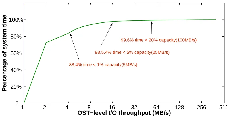
Figure 1.2 CDF of per-OST I/O throughput . . . 4

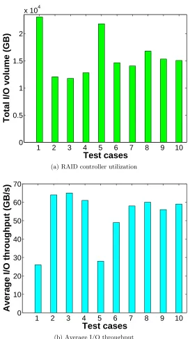
Figure 1.3 I/O performance variance test on Titan . . . 5

Figure 1.4 Sample Inter-job I/O interference . . . 7

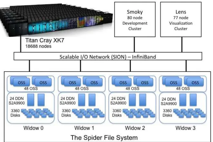
Figure 2.1 Previous Spider storage system architecture . . . 10

Figure 2.2 Current Spider storage system architecture . . . 11

Figure 2.3 Spider server-side I/O throughput . . . 13

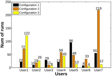
Figure 4.1 Example of the repeatability of runs on Titan, showing the number of runs using identical job configurations for seven users issuing the largest jobs, between July and September 2013. . . 18

Figure 4.2 I/O signature ofIORAand two samples . . . 20

Figure 4.3 Drift and scaling of I/O bursts across samples . . . 21

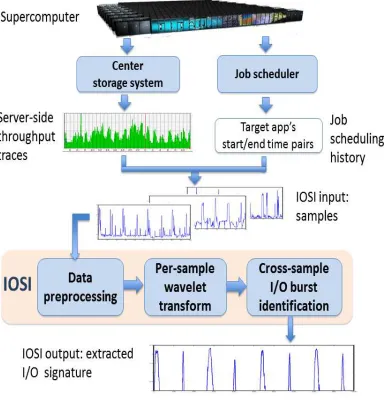
Figure 4.4 IOSI overview . . . 22

Figure 4.5 Example of outlier elimination . . . 24

Figure 4.6 IORA samples after noise reduction . . . 26

Figure 4.7 Dmey WT results on a segment ofIORAS6 . . . 27

Figure 4.8 Mapping IORA I/O bursts to 2-D points . . . 29

Figure 4.9 CLIQUE 2-D grid containingIORA bursts . . . 30

Figure 4.10 Samples fromIORA test cases . . . 32

Figure 4.11 Samples fromIORB test cases . . . 33

Figure 4.12 Samples fromIORC test cases . . . 34

Figure 4.13 Target and extracted I/O signatures of IORAtest cases . . . 35

Figure 4.14 Target and extracted I/O signatures of IORB test cases . . . 36

Figure 4.15 Target and extracted I/O signatures of IORC test cases . . . 37

Figure 4.16 S3D samples . . . 38

Figure 4.17 S3D target I/O signature and extracted I/O signature by IOSI and DTW . 39 Figure 4.18 I/O signature accuracy evaluation . . . 40

Figure 4.19 IOSI - WT sensitivity analysis . . . 42

Figure 4.20 IOSI - Clustering sensitivity analysis . . . 43

Figure 4.21 Processing time analysis . . . 44

Figure 4.22 Weak scaling sample and IOSI extracted I/O signature . . . 45

Figure 5.1 AID software architecture . . . 49

Figure 5.2 Example of OPTICS clustering . . . 53

Figure 5.3 Restructured sample based on clustering result . . . 54

Figure 5.4 Real Titan application I/O characterization accuracy . . . 62

Figure 5.5 IOR pseudo-application I/O characterization accuracy . . . 63

Figure 5.6 I/O bursts before/after OST footprint analysis . . . 65

Chapter 1

Introduction

High-performance computing (HPC) systems cater to a diverse mix of scientific applications that run concurrently. While individual compute nodes are usually dedicated to a single par-allel job at a time, the interconnection network and the storage subsystem are often shared among jobs. Network topology-aware job placement attempts to allocate larger groups of con-tiguous compute nodes to each application, in order to provide more stable message-passing performance for inter-process communication. I/O resource contention, however, continues to cause significant performance vagaries in applications [21, 80]. For example, the indispensable task of checkpointing is becoming increasingly cumbersome. The CHIMERA [18] astrophysics application produces 160TB of data per checkpoint, taking around an hour to write [46] on Titan.

This already bottleneck-prone I/O operation is further stymied by resource contention due to concurrent applications, as there is no I/O-aware scheduling or inter-job coordination on su-percomputers [85, 29, 33]. As hard disks remain the dominant parallel file system storage media, I/O contention leads to excessive seeks, significantly degrading the overall I/O throughput.

This problem is expected to exacerbate on future extreme-scale machines (hundreds of petaflops). Future systems demand a sophisticated interplay between application requirements and system software tools that is lacking in today’s systems. The aforementioned I/O perfor-mance variance problem makes an excellent candidate for such synergistic efforts. For example, knowledge of application-specific I/O behavior potentially allows a scheduler to stagger I/O-intensive jobs, improvingboth the stability of individual applications’ I/O performance and the overall resource utilization.

In this Ph.D. thesis study, for achieving such efficient I/O characterization and I/O-aware job scheduling, we propose two novel systems, IOSI (I/O Signature Identifier)[50] and AID (Automatic I/O Diverter)(Submitted for publication). IOSI is designed for automatically iden-tifying the I/O signature of data-intensive parallel applications from existing supercomputer server-side I/O traffic logs and batch job history jobs. AID takes one more step beyond: it mines I/O intensive applications from these two logs fully automatically without requiring any apriori information on the applications or jobs. Based on the automatic I/O characterization results, it further explores the potential of performing I/O-aware job scheduling. Both IOSI and AID achieve the goals without bring any extra overhead to the system, or requiring any effort from developers/users . Below we give high-level introductions on our target problems and solutions.

1.1

I/O Characterization

I/O-aware scheduling requires detailed information on application I/O characteristics, which is very challenging by itself. In this thesis work, we first explore the techniques needed to capture such information in an automatic and non-intrusive way.

Cross-layer communication regarding I/O characteristics, requirements or system status has remained a challenge. Traditionally, these I/O characteristics have been captured using client-side tracing tools [6, 8], running on the compute nodes. Unfortunately, the information provided by client-side tracing is not enough for inter-job coordination due to the following reasons.

ˆ First, client-side tracing requires the use of I/O tracing libraries and/or application code instrumentation, often requiring non-trivial development/porting effort.

ˆ Second, such tracing effort is entirely elective, rendering any job coordination ineffective when only a small portion of jobs perform (and release) I/O characteristics.

ˆ Third, many users who do enable I/O tracing choose to turn it on for shorter debug runs and off for production runs, due to the considerable performance overhead (typically between 2% and 8% [60]).

ˆ Fourth, different jobs may use different tracing tools, generating traces with different formats and content, requiring tremendous knowledge and integration.

These factors limit the usage of client-side tracing tools for development purposes [34, 47], as opposed to routine adoption in production runs or for daily operations.

Similarly, very limited server-side I/O tracing can be performed on large-scale systems, where the bookkeeping overhead may bring even more visible performance degradations. Cen-ters usually deploy only rudimentary monitoring schemes that collectaggregate workload infor-mation regarding combined I/O traffic from concurrently running applications.

In Chapter 4, we present IOSI, a novel approach to characterizing per-application I/O be-havior from noisy, zero-overhead server-side I/O throughput logs, collected without interfering with the target application’s execution. IOSI leverages the existing infrastructure in HPC cen-ters for periodically logging high-level, server-side I/O throughput. E.g., the throughput on the I/O controllers of Titan’s Spider file system [67] is recorded once every 2 seconds. Collect-ing this information has no performance impact on the compute nodes, does not require any user effort, and has minimal overhead on the storage servers. Further, the log collection traffic flows through the storage servers’ Ethernet management network, without interfering with the application I/O. Hence, we refer to our log collection as zero-overhead.

00:00 02:00 04:00 06:00 08:00 10:00 12:00 14:00 16:00 18:00 20:00 22:00 23:590

5 10 15 20

Time

Write GB/s

Figure 1.1: Average server-side, write throughput on Titan’s Spider storage (a day in November 2011).

I/O patterns, as can be seen from Figure 1.1. Therefore, the main idea of IOSI is to collect and correlate multiple samples, filter out the “background noise”, and finally identify the target application’s native I/O traffic common across them. Here, “background noise” refers to the traffic generated by other concurrent applications and system maintenance tasks. Note that IOSI is not intended to record fine-grained, per-application I/O operations. Instead, it derives an estimate of their bandwidth needs along the execution timeline to support future I/O-aware smart decision systems.

1 2 4 8 16 32 64 128 256 512 0

20% 40% 60% 80% 100%

OST−level I/O throughput (MB/s)

Percentage of system time

98.5.4% time < 5% capacity(25MB/s)

99.6% time < 20% capacity(100MB/s)

88.4% time < 1% capacity(5MB/s)

Figure 1.2: CDF of per-OST I/O throughput

1.2

I/O Aware Job Scheduling

According to our observation of large-scale HPC systems, although significant I/O performance variance is observed frequently, on average, individual pieces of hardware (such as storage server nodes and disks) are often under-utilized.

1 2 3 4 5 6 7 8 9 10 0

0.5 1 1.5 2

x 104

Test cases

Total I/O volume (GB)

(a) RAID controller utilization

1 2 3 4 5 6 7 8 9 10

0 10 20 30 40 50 60 70

Test cases

Average I/O throughput (GB/s)

(b) Average I/O throughput

Figure 1.3: I/O performance variance test on Titan

domi-nant storage media, I/O contention leads to excessive seeks, significantly degrading the overall I/O throughput. Figure 1.3 illustrates this situation, using an pseudo-application created with IOR [1], a widely used parallel I/O benchmark. It contains five I/O phases, each writing 2TB data in aggregate from 16348 processes. We repeated the execution 10 times on different days and found that while the majority of runs finish around 3210-3300 seconds, two of them took sig-nificantly longer, with the worst one taking 4348 seconds. By checking the server-side aggregate I/O throughput during these execution time windows (Figure 1.3a), we found that the signifi-cantly delayed runs correlate with highly elevated overall system bandwidth levels (the 1st and 6th bars), while the other “normal” runs encounter concurrent traffic at a small fraction of the system peak bandwidth. The perceived aggregate I/O throughput for this pseudo-application varies accordingly (Figure 1.3b), from 26.5GB/s to 64.1GB/s. As the 10 runs produce identical I/O traffic, these results clearly demonstrate the impact of “background” I/O activities (from other concurrently running jobs and interactive use) on an individual job.

One major reason for such I/O-induced, large performance variance is the I/O-oblivious job scheduling used in current systems: on HPC systems like Titan (where the tests were conducted) job requests are served in a first-in, first-out (FIFO) order plus backfilling, with further adjustment using priorities, such as job size, queue type, and usage history [3].To our best knowledge, I/O behavior/pattern has never been taken into account in production HPC

systems’ parallel job scheduling.

One might wonder that with such an overall under-utilized storage system, I/O-intensive jobs can naturally be spaced apart by the batch queue. To check whether this is the case, we conducted tests using applications created with IOR. We defined a set of 7 pseudo-applications, TEST1 - TEST7, each with different configurations, such as node count (64 to

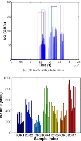
1024), total I/O volume (3 to 100TB), and computation-to-I/O ratio (4% to 20%). We submitted the set of pseudo-applications to the batch scheduler together and repeated such test several times within a week in June 2015. The average queue wait time for each job was over 10 hours. Figure 1.4a gives a segment of the aggregate server-side I/O traffic data on one Spider partition, captured on 06/13/2015. We highlight the duration of each IOR job with a color rectangle. Though the jobs were queued for much longer than their execution times, their start times were not sufficiently staggered, resulting in remarkable (yet inconsistent) I/O performance variation. Figure 1.4b shows the large distribution of total I/O time across different trials.E.g., the shortest I/O time for TEST4 was 283s, while the longest 856s (around 200% longer).

0 0.5 1 1.5 2 2.5 3 3.5 x 104 0

50 100 150 200

Time (s)

I/O (GB/s)

(a) I/O traffic with job durations

IOR1 IOR2 IOR3 IOR4 IOR5 IOR6 IOR7 0

200 400 600 800 1000

Sample index

I/O time (secs)

(b) Job I/O time

Figure 1.4: Sample Inter-job I/O interference

characteristics through tracing/profiling, and is not practical for a supercomputer/cluster to demand such information from application users or developers.

characterization and I/O-aware job scheduling. AID analyzes existing I/O traffic and batch job history logs, without any application-related prior knowledge or user/developers involvement. As the extension work of IOSI, AID is based on the same intuition: the common behavior ob-served across multiple executions of the same application is likely attributed to this application. However, IOSI identifies the I/O signature of a given I/O-intensive application and assumes its job run instances are identical executions. In contrast, AID takes a fully data-driven ap-proach, sifting out dozens of I/O-heavy applications from job-I/O history containing millions of jobs running thousands of unique applications. These applications can then be given special attention in scheduling to reduce I/O contention. Also, AID utilizes detailed per-OST logs that became available more recently, while the prior work studies aggregate traffic only.

AID correlates the coarse-grain server-side I/O traffic log (both aggregate and OST-level) to (1) identify I/O-intensive applications, (2) “mine” the I/O traffic pattern of applications classified as I/O-intensive, and (3) provide suggestions to the batch job scheduler (regarding whether an I/O-intensive job can be immediately dispatched). Note that AID achieves the above fully automatically,without requiring any apriori information on the applications or jobs. It examines the full job log and identifies common I/O patterns across the multiple executions of the same application.

1.3

Contributions

(1) To our best knowledge, this work is the first to explore log-based, automatic HPC application I/O characterization. To this end, we propose and implement IOSI, a tool that identifies given applications I/O signature using existing, zero-overhead, server-side I/O measurements and job scheduling history. Further, we obtain such knowledge of a target application without interfer-ing with its computation and communication, or requirinterfer-ing developers/users’ intervention. We evaluated IOSI with real-world server-side I/O throughput logs from the Spider storage sys-tem at the Oak Ridge Leadership Computing Facility (OLCF). Our experiments used several pseudo-applications, constructed with the expressive IOR benchmarking tool, and S3D [77], a large-scale turbulent combustion code. Our results show that IOSI effectively extracts an application’s I/O signature despite significant server-side noises.

of I/O-intensive jobs dispatched upon different AID suggestions (“run” or “delay”). Our results confirm that AID can successfully identify I/O-intensive applications and their high-level I/O characteristics. In addition, while we currently do not have means to deploy new scheduling policies on Titan, our proof-of-concept evaluation indicates that I/O-aware scheduling might be highly promising for future supercomputing systems.

1.4

Dissertation Outline

Chapter 2

Background

Our work targets petascale or larger platforms, motivated by their extensive storage-side mon-itoring framework. Below we give a big picture of one such storage system, the ORNL Spider file system [76], supporting Titan and several other clusters.

2.1

Titan’s Spider Storage Infrastructure

Our prototype development and evaluation use the storage server statistics collected from the Spider center-wide storage system [76] at OLCF, a Lustre-based parallel file system. Spider currently serves the world’s No. 2 machine, the 27 petaflop Titan, in addition to other smaller development and visualization clusters. Notice that since Spider has been upgraded to a more powerful system at the beginning of 2014, our IOSI work is based on the previous version of Spider while AID is based on the upgraded system.

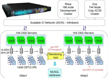
Figure 2.1 shows the previous Spider architecture, which comprises of 96 Data Direct Net-works (DDN) S2A9900 RAID controllers, with an aggregate bandwidth of 240 GB/s and over 10 PBs of storage from 13,440 1-TB SATA drives. Access is through the object storage servers (OSSs), connected to the RAID controllers in a fail-over configuration. The compute platforms connect to the storage infrastructure over a multistage InfiniBand network, SION (Scalable I/O Network). Spider has four partitions, widow[0−3], with identical setup and capacity.

Figure 2.2: Current Spider storage system architecture

Lustre Object Storage Servers (OSSs), each with 7 OSTs attached, partitioned into two inde-pendent and non-overlapping namespaces, atlas1 and atlas2, for load-balancing and capacity management. Each partition includes half of the system: 144 Lustre OSSs and 1,008 OSTs. The compute nodes (clients) connect to Spider over a multistage InfiniBand network (SION).

2.2

I/O and Job Data Collection

I/O traffic log Server-side I/O statistics has been collected since 2009 on Spider, via a custom API provided by the DDN controllers. A custom daemon utility [59] polls the controllers periodically and stores the results in a MySQL database. Data collected include read/write I/O throughput and IOPS, I/O request sizes, etc., amounting typically around 4GB log data per day. Unlike client-side or server-side I/O tracing, such coarse-grained monitoring/logging collected over the management Ethernet network (separate from application data traffic) has negligible overhead.

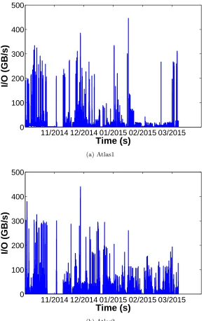
Figure 2.3 shows the aggregated I/O throughput from the two Spider partitions between

2014-11-01 and2015-03-31. The observed peak I/O throughput is close to the theoretical peak, around 500 GB/s per partition [65]. However, for most of the time, the I/O throughput is much lower. Also, notable lapses in I/O activity correlated well with recorded system maintenance windows or interruptions to the data collection process. In addition, the two partitions were not utilized equally, with free space onatlas2 over 40% higher than onatlas1 (the default partition) in June 2015.

Applications are allocated a set of OSTs. Based on thestripe width k, the I/O client round robins across the k OST s. The current Spider has monitoring tools capturing per-OST I/O activity. In this work, we leverage this OST-level information for I/O pattern mining and scheduling.

11/2014 12/2014 01/2015 02/2015 03/2015 0

100 200 300 400 500

Time (s)

I/O (GB/s)

(a) Atlas1

11/2014 12/2014 01/2015 02/2015 03/2015 0

100 200 300 400 500

Time (s)

I/O (GB/s)

(b) Atlas2

Chapter 3

Related Work

3.1

I/O Access Patterns

Miller and Katz observed that scientific I/O has highly sequential and regular accesses, with a period of CPU processing followed by an intense, bursty I/O phase [31]. Carns et al. noted that HPC I/O patterns tend to be repetitive across different runs, suggesting that I/O logs from prior runs can be a useful resource for predicting future I/O behavior [21]. Similar claims have been made by other studies on the I/O access patterns of scientific applications [36, 63, 74]. Such studies strongly motivate IOSI’s attempt to identify common and distinct I/O bursts of an application from multiple noisy, server-side logs.

Prior work has also examined the identification and use of I/O signatures. For example, the aforementioned work by Carns et al. proposed a methodology for continuous and scalable characterization of I/O activities [21]. Byna and Chen also proposed an I/O prefetching method with runtime and post-run analysis of applications’ I/O signatures [20]. A significant difference is that IOSI is designed to automatically extract I/O signatures from existing coarse-grained server-side logs, while prior approaches for HPC rely on client-side tracing (such as MPI-IO instrumentation). For more generic application workload characterization, a few studies [72, 78, 87] have successfully extracted signatures from various server-side logs.

3.2

Client-side I/O Tracing Tools

A number of tools have been developed for general-purpose client-side instrumentation, profil-ing, and tracing of generic MPI and CPU activity, such as mpiP [81], LANL-Trace [2], HPCT-IO [75], and TRACE [58]. The most closely related to HPCT-IOSI is probably Darshan [22]. It performs low-overhead, detailed I/O tracing and provides powerful post-processing of log files. It outputs a large collection of aggregate I/O characteristics such as operation counts and request size his-tograms. However, existing client-side tracing approaches suffer from the limitations mentioned in Chapter 1.1, such as installation/linking requirements, voluntary participation, and produc-ing additional client I/O traffic. Our server-side approach allows us to handle applications usproduc-ing any I/O interface.

3.3

Time-series Data Alignment

There have been many studies in this area [7, 13, 14, 35, 49, 62]. Among them, dynamic time warping (DTW) [14, 62] is a well-known approach for comparing and averaging a set of se-quences. Originally, this technique was widely used in the speech recognition community for automatic speech pattern matching [28]. Recently, it has been successfully adopted in other areas, such as data mining and information retrieval, for automatically addressing time defor-mations and aligning time-series data [23, 38, 42, 90]. Due to its maturity and existing adoption, we choose DTW for comparison against the IOSI algorithms.

3.4

Resource-aware job scheduling

Chapter 4

I/O Signature Identifier

4.1

Background

We first describe the features of typical I/O-intensive parallel applications on supercomputers, which partially enable IOSI.

The majority of applications on today’s supercomputers are parallel numerical simulations that perform iterative, timestep-based computations. These applications are write-heavy, peri-odically writing out intermediate results and checkpoints for analysis and resilience, respectively. For instance, applications compute for a fixed number of timesteps and then perform I/O, re-peating this sequence multiple times. This process creates regular, predictable I/O patterns, as noted by many existing studies [31, 68, 83]. More specifically, parallel applications’ dominant I/O behavior exhibits several distinct features that enable I/O signature extraction:

Burstiness:Scientific applications have distinct compute and I/O phases. Most applications are designed to perform I/O in short bursts [83].

Periodicity:Most I/O-intensive applications write data periodically, often in a highly reg-ular manner [31, 68] (both in terms of interval between bursts and the output volume per burst). Such regularity and burstiness suggests the existence of steady, wavelike I/O signatures. Note that although a number of studies have been proposed to optimize the checkpoint inter-val/volume [24, 25, 51], regular, content-oblivious checkpointing is still the standard practice in large-scale applications [70, 89]. IOSI does not depend on such periodic I/O patterns and han-dles irregular patterns, as long as the application I/O behavior stays consistent across multiple job runs.

User1 User2 User3 User4 User5 User6 User7 0

50 100 150 200 250

22

72

122

10

19

26

₂₉

11

₈

21

58

45

96

48

13

₈

33

6

55

219

12

Users

Num of runs

Configuration 1 Configuration 2 Configuration 3

Figure 4.1: Example of the repeatability of runs on Titan, showing the number of runs using identical job configurations for seven users issuing the largest jobs, between July and September 2013.

studied three years worth of Spider server-side I/O throughput logs and Titan job traces for the same time period, and verified that applications have a recurring I/O pattern in terms of frequency and I/O volume. Figure 4.1 plots statistics of per-user jobs using identical job configurations, which is highly indicative of executions of the same application. We see that certain users, especially those issuing large-scale runs, tend to reuse the same job configuration for many executions.

4.2

Problem Definition: Parallel Application I/O Signature

Iden-tification

As mentioned earlier, IOSI aims to identify the I/O signature of a parallel application, from zero-overhead, aggregate, server-side I/O throughput logs that are already being collected. IOSI’s input includes (1) the start and end times of the target application’s multiple executions in the past, and (2) server-side logs that contain the I/O throughput generated by those runs (as well as unknown I/O loads from concurrent activities). The output is the extracted I/O signature of the target application.

We define an application’s I/O signature as the I/O throughput it generates at the server-side storage of a given parallel platform, for the duration of its execution. In other words, if this application runs alone on the target platform without any noise from other concurrent jobs or interactive/maintenance workloads, the server-side throughput log during its execution will be its signature. It is virtually impossible to find such “quiet time” once a supercomputer enters the production phase. Therefore, IOSI needs to “mine” the true signature of the application from server-side throughput logs, collected from its multiple executions. Each execution instance, however, will likely contain different noise signals. We refer to each segment of such a noisy server-side throughput log, punctuated by the start and end times of the execution instance, a “sample”. Based on our experience, generally 5 to 10 samples are required for getting the expected results. Note that there are long-running applications (potentially several days for each execution). It is possible for IOSI to extract a signature from even partial samples (e.g., from one tenth of an execution time period), considering the self-repetitive I/O behavior of large-scale simulations.

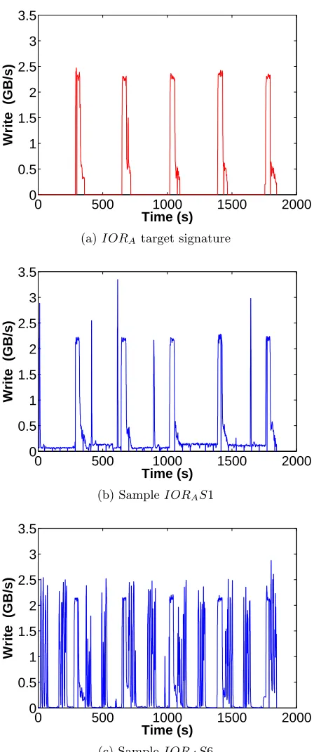
Figure 4.2 illustrates the signature extraction problem using a pseudo-application, IORA,

generated by IOR. IOR supports most major HPC I/O interfaces (e.g., POSIX, MPIIO, HDF5), provides a rich set of user-specified parameters for I/O operations (e.g., file size, file sharing setting, I/O request size), and allows users to configure iterative I/O cycles. IORA exhibits a

0 500 1000 1500 2000 0

0.5 1 1.5 2 2.5 3 3.5

Time (s)

Write (GB/s)

(a)IORA target signature

0 500 1000 1500 2000 0

0.5 1 1.5 2 2.5 3 3.5

Time (s)

Write (GB/s)

(b) SampleIORAS1

0 500 1000 1500 2000 0

0.5 1 1.5 2 2.5 3 3.5

Time (s)

Write (GB/s)

(c) SampleIORAS6

4.3

Challenges and Approach Overview

Thematic to IOSI is the realization that the noisy, server-side samples contain common, periodic I/O bursts of the target application. It exploits this fact to extract the I/O signature, using a rich set of statistical techniques. Simply correlating the samples is not effective in extracting per-application I/O signatures, due to a set of challenges detailed below.

0 200 400 600 800 1000 1200 1400

0 0.5 1 1.5 2 2.5 3

Time (s)

Write (GB/s)

Sample 1 Sample 2

Figure 4.3: Drift and scaling of I/O bursts across samples

following dilemma in processing the I/O signals: IOSI has to rely on the application’s I/O bursts to properlyalign the noisy samples as they are the only common features; at the same time, it needs the samples to be reasonably aligned toidentify the common I/O bursts as belonging to the target application.

Figure 4.4: IOSI overview

tools to discover the target application’s I/O signature using a black-box approach, unlike prior work based on white-box models [22, 80]. Recall that IOSI’s purpose is to render a reliable estimate of user-applications’ bandwidth needs, instead of to optimize individual applications’ I/O operations. Black-box analysis is better suited here for generic and non-intrusive pattern collection.

The overall context and architecture of IOSI are illustrated in Figure 4.4. Given a target application, multiple samples from prior runs are collected from the server-side logs. Using such a sample set as input, IOSI outputs the extracted I/O signature by mining the common characteristics hidden in the sample set. Our design comprises of three phases:

1. Data preprocessing: This phase consists of four key steps: outlier elimination, sample granularity refinement, runtime correction, and noise reduction. The purpose is to prepare the samples for alignment and I/O burst identification.

2. Per-sample wavelet transform: To utilize “I/O bursts” as common features, we employ wavelet transform to distinguish and isolate individual bursts from the noisy background.

3. Cross-sample I/O burst identification: This phase identifies the common bursts from multiple samples, using a grid-based clustering algorithm.

4.4

IOSI Design and Algorithms

In this section, we describe IOSI’s workflow, step by step, using the aforementioned IORA

pseudo-application (Figure 4.2) as a running example.

4.4.1 Data Preprocessing

Given a target application, we first compare the job log with the I/O throughput log, to obtain I/O samples from the application’s multiple executions, particularlyby the same user and with

the same job size (in term of node counts). As described in Chapter 4.1, HPC users tend to run their applications repeatedly.

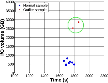
From this set, we then eliminate outliers – samples with significantly heavier noise signals or longer/shorter execution time.1 Our observation from Spider is that despite unpredictable noise, the majority of the samples (from the same application) bear considerable similarity. Intuitively, including the samples that are apparently significantly skewed by heavy noise is counter-productive. We performoutlier elimination by examining (1) the application execution time and (2) the volume of data written within the sample (the “area” under the server-side

1

10000 1200 1400 1600 1800 2000 2200 500

1000 1500 2000 2500 3000 3500 4000

Time (s)

I/O volume (GB)

Normal sample Outlier sample

Figure 4.5: Example of outlier elimination

throughput curve). Within this 2-D space, we apply the Local Outlier Factor (LOF) algo-rithm [17], which identifies observations beyond certain threshold as outliers. Here we set the thresholdµ as the mean of the sample set. Figure 4.5 illustrates the distribution of execution times and I/O volumes among 10IORAsamples collected on Spider, where two of the samples

(dots within the circle) are identified by LOF as outliers.

Next, we perform sample granularity refinement, by decreasing the data point interval from 2 seconds to 1 using simple linear interpolation [27]. Thus, we insert an extra data point between two adjacent ones, which turns out to be quite helpful in identifying short bursts that last for only a few seconds. The value of each extra data point is the average value of its adjacent data points. It is particularly effective in retaining the amplitude of narrow bursts during the subsequent WT stage.

discards data points at regular intervals to shrink each longer sample to match the shortest one. For example, if a sample is 4% longer than the shortest one, then we remove from it the 1st, 26th, 51st, ..., data points. We found that after outlier elimination, the deviation in sample duration is typically less than 10%. Therefore such trimming is not expected to significantly affect the sample data quality.

Finally, we perform preliminary noise reduction to remove background noise. While I/O-intensive applications produce heavy I/O bursts, the server-side log also reports I/O traffic from interactive user activities and maintenance tasks (such as disk rebuilds or data scrubbing by the RAID controllers). Removing this type of persistent background noise significantly helps signature extraction. In addition, although such noise does not significantly distort the shape of application I/O bursts, having it embedded (and duplicated) in multiple application’s I/O signatures will cause inaccuracies in I/O-aware job scheduling. To remove background noise, IOSI (1) aggregates data points from all samples, (2) collects those with a value lower than the overall average throughput, (3) calculates the average background noise level as the mean throughput from these selected data points, and (4) lowers each sample data point by this average background noise level, producing zero if the result is negative. Figure 4.6b shows the result of such preprocessing, and compared to the original sample in Figure 4.6a, the I/O bursts are more pronounced. The I/O volume ofIORAS1 was trimmed by 26%, while the background

noise level was measured at 0.11 GB/s.

4.4.2 Per-Sample Wavelet Transform

As stated earlier, scientific applications tend to have a bursty I/O behavior, justifying the use ofI/O burst as the basic unit of signature identification. An I/O burst indicates a phase of high I/O activity, distinguishable from the background noise over a certain duration.

With less noisy samples, the burst boundaries can be easily found using simple methods such as first difference [69] or moving average [84]. However, with noisy samples identifying such bursts becomes challenging, as there are too many ups and downs close to each other. In particular, it is difficult to do so without knowing the cutoff threshold for a “bump” to be considered a candidate I/O burst. Having too many or too few candidates can severely hurt our sample alignment in the next step.

To this end, we use a WT [26, 57, 86] to smooth samples. WT has been widely applied to problems such as filter design [19], noise reduction [45], and pattern recognition [30]. With WT, a time-domain signal can be decomposed into low-frequency and high-frequency components. The approximation information remains in the low-frequency component, while the detail in-formation remains in the high-frequency one. By carefully selecting the wavelet function and

0

500

1000

1500

2000

0

0.5

1

1.5

2

2.5

3

3.5

Time (s)

Write (GB/s)

(a) Before noise reduction

0

500

1000

1500

2000

0

0.5

1

1.5

2

2.5

3

3.5

Time (s)

Write (GB/s)

(b) After noise reduction

Figure 4.6: IORAsamples after noise reduction

contain the most energy of the signal and are isolated from the background noise.

characteristics of the time-series sample.

WT can use quite a few wavelet families [5, 61], such as Haar, Daubechies, and Coiflets. Each provides a transform highlighting different frequency and temporal characteristics. For IOSI, we choose discrete Meyer (dmey) [54] as the mother wavelet. Due to its smooth profile, the approximation part of the resulting signal consists of a series of smooth waves. Its output consists of a series of waves where the center of the wave troughs can be easily identified as wave boundaries.

0 200 400 600 800

0 0.5 1 1.5 2 2.5 3 Time (s) Write (GB/s)

(a) PreprocessedIORAS6 segment

0 200 400 600 800

0 0.5 1 1.5 2 2.5 3 Time (s) Write (GB/s)

(b) After WT (Decomposition level 1)

0 200 400 600 800

0 0.5 1 1.5 2 2.5 3 Time (s) Write (GB/s)

(c) After WT (Decomposition level 2)

0 200 400 600 800

0 0.5 1 1.5 2 2.5 3 Time (s) Write (GB/s)

(d) After WT (Decomposition level 3)

Figure 4.7: Dmey WT results on a segment ofIORAS6

Figures 4.7a and Figures 4.7b, 4.7c, 4.7d illustrate a segment ofIORAS6 and its dmey WT

from the application’s point of view may appear to have many “sub-crests”, separated by minor troughs. This is due to throughput variance caused by either application behavior (such as adjacent I/O calls separated by short computation/communication) or noise, or both. To prevent creating many such “sub-bursts”, we use the mean height of all wave crests for filtering – only the troughs lower than this threshold are used for separating bursts.

Another WT parameter to consider is the decomposition level, which determines the level of detailed information in the results. The higher the decomposition level, the fewer details are shown in the low-frequency component, as can be seen from Figures 4.7b, 4.7c and 4.7d. With a decomposition level of 1 (e.g. Figures 4.7b), the wavelet smoothing is not sufficient for isolating burst boundaries. With a higher decomposition level of 3 the narrow bursts fade out rapidly, potentially missing target bursts. IOSI uses a decomposition level of 2 to better retain the bursty nature of the I/O signature.

4.4.3 Cross-Sample I/O Burst Identification

Next, IOSI correlates all the pre-processed, and wavelet transformed samples to identify com-mon I/O bursts. To address the circular dependency challenge mentioned earlier between align-ment and common feature identification, we adapt a grid-based clustering approach called CLIQUE [9]. It performs multi-dimensional data clustering by identifying grids (called units) where there is higher density (number of data points within the unit). CLIQUE treats each such dense unit as a “seed cluster” and grows it by including neighboring dense units.

CLIQUE brings several advantages to IOSI. First, its model fits well with our context: an I/O burst from a given sample is mapped to a 2-D data point, based on itstimeandshapeattributes. Therefore, data points from different samples close to each other in the 2-D space naturally indicate common I/O bursts. Second, with controllable grid width and height, IOSI can better handle burst drifts (more details given below). Third, CLIQUE performs well for scenarios with far-apart clusters, where inter-cluster distances significantly exceed those between points within a cluster. As parallel applications typically limit their “I/O budget” (fraction of runtime allowed for periodic I/O) to 5%-10%, individual I/O bursts normally last seconds to minutes, with dozens of minutes between adjacent bursts. Therefore, CLIQUE is not only effective for IOSI, but also efficient, as we do not need to examine too far around the burst-intensive areas. Our results (Chapter 4.5) show that it outperforms the widely used DTW time-series alignment algorithm [14], while incurring significantly lower overhead.

Figure 4.8: Mapping IORAI/O bursts to 2-D points

in a unit, but on the number of different samples with bursts there. The intuition is that a common burst from the target application should have most (if not all) samples agree on its existence. Below, we illustrate with IORAthe process of IOSI’s common burst identification.

To use our adapted CLIQUE, we need to first discretize every samplesi into a group of 2-D

points, each representing one I/O burst identified after a WT. Given itsjth I/O burstbi,j, we

map it to point hti,j, ci,ji. Here ti,j is the time of the wave crest of bi,j, obtained after a WT,

while ci,j is the correlation coefficient between bi,j and a reference burst. To retain the details

describing the shape of the I/O burst, we choose to use the pre-WT burst in calculating ci,j,

though the burst itself was identified using a WT. Note that we rely on the transitive nature of correlation (“bursts with similar correlation coefficient to the common reference burst tend to be similar to each other”), so the reference burst selection does not have a significant impact on common burst identification. In our implementation, we use the “average burst” identified by WT across all samples.

Figure 4.8 shows how we mapped 4 I/O bursts, each from a different IORA sample. Recall

Figure 4.9: CLIQUE 2-D grid containingIORA bursts

selected width and height values, there is still a chance that a cluster of nodes are separated into different grids, causing CLIQUE to miss a dense unit.

To this end, instead of using only one pair of width-height values, IOSI tries out multiple grid size configurations, each producing an extracted signature. For width, it sets the lower bound as the average I/O burst duration across all samples and upper bound as the average time distance between bursts. For a unit height, it empirically adopts the range between 0.05 and 0.25. Considering the low cost of CLIQUE processing with our sample sets, IOSI uniformly samples this 2-D parameter space (e.g., with 3-5 settings per dimension), and takes the result that identified the most data points as belonging to common I/O bursts. Due to the strict requirement of identifying common bursts, we have found in our experiments that missing target bursts is much more likely to happen than including fake bursts in the output signature. Figure 4.9 shows the resulting 2-D grid, containing points mapped from bursts in four IORA

samples.

We have modified the originaldense unit definition as follows. Givenssamples, we calculate the density of a unit as “the number of samples that have points within this unit”. If a unit meets a certain density threshold dγ∗se, whereγ is a controllable parameter between 0 and 1, the unit is considered dense. Our experiments used a γ value of 0.5, requiring each dense unit to have points from at least 2 out of the 4 samples. All dense units are marked with a dark shade in Figure 4.9.

dense unit, we only check its immediate neighborhood (shown in a lighter shade in Figure 4.9) for data points potentially from a common burst. We identify dense neighborhoods (including the central dense unit) as those meeting a density threshold of dκ∗se, where κ is another configurable parameter with value larger thanγ (e.g., 0.9).

Note that it is possible for the neighborhood (or even a single dense unit) to contain multiple points from the same sample. IOSI further identifies points from the common I/O burst using a voting scheme. It allows up to one point to be included from each sample, based on the total normalized Euclidean distance from a candidate point to peers within the neighborhood. From each sample, the data point with the lowest total distance is selected. In Figure 4.9, the neighborhood of dense unit 5 contains two bursts fromIORAS3 (represented by dots). The

burst in the neighborhood unit (identified by the circle) is discarded using our voting algorithm. As the only “redundant point” within the neighborhood, it is highly likely to be a “fake burst” from other concurrently running I/O-intensive applications. This can be confirmed by viewing the original sampleIORAS3 in Figure4.10b, where a tall spike not fromIORAshows up around

the 1200th second.

4.4.4 I/O Signature Generation

Given the common bursts from dense neighborhoods, we proceed to sample alignment. This is done by aligning all the data points in a common burst to the average of theirxcoordinate val-ues. Thereafter, we generate the actual I/O signature by sweeping along thex(time) dimension of the CLIQUE 2-D grid. For each dense neighborhood identified, we generate a corresponding I/O burst at the aligned time interval, by averaging the bursts mapped to the selected data points in this neighborhood. Here we used the bursts after preprocessing, but before WT.

4.5

Experimental Evaluation

4.5.1 IOSI Experimental Evaluation

We have implemented the proof-of-concept IOSI prototype using Matlab and Python. To val-idate IOSI, we used IOR to generate multiple pseudo-applications with different I/O write patterns, emulating write-intensive scientific applications. In addition, we used S3D [39, 77], a massively parallel direct numerical simulation solver developed at Sandia National Laboratory for studying turbulent reacting flows.

Figure 4.13a, 4.14a and 4.15a are the true I/O signatures of the three IOR pseudo-applications, IORA, IORB, and IORC. These pseudo-applications were run on the Smoky

0 400 800 1200 1600 2000 0 0.5 1 1.5 2 2.5 3 3.5 4 4.5 Time (s) Write (GB/s)

(a)IORAS1

0 400 800 1200 1600 2000 0 0.5 1 1.5 2 2.5 3 3.5 4 4.5 Time (s) Write (GB/s)

(b)IORAS2

0 400 800 1200 1600 2000 0 0.5 1 1.5 2 2.5 3 3.5 4 4.5 Time (s) Write (GB/s)

(c)IORAS3

0 400 800 1200 1600 2000 0 0.5 1 1.5 2 2.5 3 3.5 4 4.5 Time (s) Write (GB/s)

(d)IORAS4

Figure 4.10: Samples fromIORA test cases

MPI-IO. We were able to obtain “clean” signatures (with little noise) for these applications by running our jobs when Titan was not in production use (under maintenance) and one of the file system partitions was idle. Among them, IORA represents simple periodic checkpointing,

writing the same volume of data at regular intervals (128GB every 300s). IORB also writes

periodically, but alternates between two levels of output volume (64GB and 16GB every 120s), which is typical of applications with different frequencies in checkpointing and results writing (e.g., writing intermediate results every 10 minutes but checkpointing every 30 minutes).IORC

0 200 400 600 800 1000 1200 0 1 2 3 4 5 Time (s) Write (GB/s)

(a)IORBS1

0 200 400 600 800 1000 1200 0 1 2 3 4 5 Time (s) Write (GB/s)

(b)IORBS2

0 200 400 600 800 1000 1200 0 1 2 3 4 5 Time (s) Write (GB/s)

(c)IORBS3

0 200 400 600 800 1000 1200 0 1 2 3 4 5 Time (s) Write (GB/s)

(d)IORBS4

Figure 4.11: Samples from IORB test cases

IOR Pseudo-Application Results

To validate IOSI, the IOR pseudo-applications were run at different times of the day, over a two-week period. Each application was run at least 10 times. During this period, the file system was actively used by Titan and other clusters. The I/O activity captured during this time is the noisy server-side throughput logs. From the scheduler’s log, we identified the execution time intervals for the IOR runs, which were then intersected with the I/O throughput log to obtain per-application samples.

0 400 800 1200 1600 2000 0 1 2 3 4 5 6 Time (s) Write (GB/s)

(a)IORCS1

0 400 800 1200 1600 2000

0 1 2 3 4 5 6 Time (s) Write (GB/s)

(b)IORCS2

0 400 800 1200 1600 2000

0 1 2 3 4 5 6 Time (s) Write (GB/s)

(c)IORCS3

0 400 800 1200 1600 2000

0 1 2 3 4 5 6 Time (s) Write (GB/s)

(d)IORCS4

Figure 4.12: Samples from IORC test cases

application is much higher (say 20GB/s), the problem becomes much easier, since there is less background noise that can achieve that bandwidth level to interfere.

Due to the space limit, we only show four samples for each pseudo-app in Figure 4.10, 4.11 and 4.12. We observe that most of them show human-visible repeated patterns that overlap with the target signatures. There is, however, significant difference between the target signa-ture and any individual sample. The samples show a non-trivial amount of “random” noise, sometimes (e.g.,IORAS1) with distinct “foreign” repetitive pattern, most likely from another

0 500 1000 1500 2000 0 0.5 1 1.5 2 2.5 3 Time (s)

Write (GB/s)

(a)IORAtarget signature

0 500 1000 1500 2000

0 0.5 1 1.5 2 2.5 3 Time (s) Write (GB/s)

(b) IOSI w/o data preprocessing

0 500 1000 1500 2000

0 0.5 1 1.5 2 2.5 3 Time (s) Write (GB/s)

(c) IOSI with data preprocessing

0 500 1000 1500 2000

0 0.5 1 1.5 2 2.5 3 Time (s) Write (GB/s)

(d) DTW with data preprocessing

Figure 4.13: Target and extracted I/O signatures of IORA test cases

signature extraction).

Figure 4.13, 4.14 and 4.15 presents the original signatures and the extracted signatures using three approaches: IOSI with and w/o data preprocessing, plus DTW with data preprocessing. As introduced in Chapter 3, DTW is a widely used approach for finding the similarity between two data sequences. In our problem setting, similarity means a match in I/O bursts from two samples. We used sample preprocessing to make a fair comparison between DTW and IOSI. Note that IOSI without data preprocessing utilizes samples after granularity refinement, to obtain extracted I/O signatures with similar length across all three methods tested.

0 200 400 600 800 1000 0 0.5 1 1.5 2 2.5 3 3.5 Time (s)

Write (GB/s)

(a)IORB target signature

0 200 400 600 800 1000

0 0.5 1 1.5 2 2.5 3 Time (s) Write (GB/s)

(b) IOSI w/o data preprocessing

0 200 400 600 800 1000

0 0.5 1 1.5 2 2.5 3 Time (s) Write (GB/s)

(c) IOSI with data preprocessing

0 200 400 600 800 1000

0 0.5 1 1.5 2 2.5 3 Time (s) Write (GB/s)

(d) DTW with data preprocessing

Figure 4.14: Target and extracted I/O signatures ofIORB test cases

the alternative of averaging all pair-wise DTW results, since it implicitly carries out global data alignment. Still, DTW generated significantly lower-quality signatures, especially with more complex I/O patterns, due to its inability to reduce noise. For example, DTW’s IORC

(Figure 4.15d) signature appears to be dominated by noise.

0 500 1000 1500 0 0.5 1 1.5 2 2.5 3 3.5 Time (s)

Write (GB/s)

(a)IORCtarget signature

0 500 1000 1500 0 1 2 3 4 Time (s) Write (GB/s)

(b) IOSI w/o data preprocessing

0 500 1000 1500 0 1 2 3 4 Time (s) Write (GB/s)

(c) IOSI with data preprocessing

0 500 1000 1500 0 1 2 3 4 Time (s) Write (GB/s)

(d) DTW with data preprocessing

Figure 4.15: Target and extracted I/O signatures ofIORC test cases

S3D Results

0 800 1600 2400 0 2 4 6 8 10 12 14 Time (s) Write (GB/s)

(a)S3DS1

0 800 1600 2400

0 2 4 6 8 10 12 14 Time (s) Write (GB/s)

(b)S3DS2

0 800 1600 2400

0 2 4 6 8 10 12 14 Time (s) Write (GB/s)

(c)S3DS3

0 800 1600 2400

0 2 4 6 8 10 12 14 Time (s) Write (GB/s)

(d)S3DS4

Figure 4.16: S3D samples

0 1000 2000 3000 0 2 4 6 8 10 Time (s) Write (GB/s)

(a) S3D target I/O signature

0 1000 2000 3000

0 2 4 6 8 10 Time (s) Write (GB/s)

(b) IOSI w/o data preprocessing

0 1000 2000 3000

0 2 4 6 8 10 Time (s) Write (GB/s)

(c) IOSI with data preprocessing

0 1000 2000 3000

0 2 4 6 8 10 Time (s) Write (GB/s)

(d) DTW with data preprocessing

Figure 4.17: S3D target I/O signature and extracted I/O signature by IOSI and DTW

4.5.2 Accuracy and Efficiency Analysis

We quantitatively compare the accuracy of IOSI and DTW using two commonly used similarity metrics, cross correlation (Figure 4.18a) and correlation coefficient (Figure 4.18b). Correlation coefficient measures the strength of the linear relationship between two samples. Cross cor-relation [88] is a similarity measurement that factors in the drift in a time series data set. Figure 4.18 portraits these two metrics, as well as the total I/O volume comparison, between the extracted and the original application signature.

Note that correlation coefficient is inadequate to characterize the relationship between the two time series when they are not properly aligned. For example, with IORB, the number

0 0.2 0.4 0.6 0.8 1 0.940.95 0.35 0.87 0.52 0.38 0.8 0.34 0.38 0.72 0.39 0.28 Test case Cross Correlation IOR

A IORB IORC S3D

IOSI w data preprocessing IOSI w/o data preprocessing DTW with data preprocessing

(a) Cross correlation

0 0.2 0.4 0.6 0.8

1 0.94 0.95

0.15 0.69 0.16 0.15 0.75 0.13 0.1 0.66 0.12 0 Test case Correlation coefficient IOR

A IORB IORC S3D

IOSI w data preprocessing IOSI w/o data preprocessing DTW with data preprocessing

(b) Correlation coefficient

0 200 400 600 800 1000 1200 352396 668 510 157 127 287 196 406408 770 516 384 370 454 389 Test case

Total I/O Volume (GB)

IOR

A IORB IORC S3D

IOSI w data preprocessing IOSI w/o data preprocessing DTW with data preprocessing Target signature

(c) Total I/O volume

signature. Cross correlation appears more tolerant to IOSI without preprocessing compared to correlation coefficient. Also, IOSI significantly outperforms DTW (both with preprocessing), by a factor of 2.1-2.6 in cross correlation, and 4.8-66.0 in correlation coefficient.

Note that the DTW correlation coefficient for S3D is too small to show. Overall, IOSI with preprocessing achieves a cross correlation between 0.72 and 0.95, and a correlation coefficient between 0.66 and 0.94.

We also compared the total volume of I/O traffic (i.e., the “total area” below the signature curve), shown in Figure 4.18c. IOSI generates I/O signatures with a total I/O volume closer to the original signature than DTW does. It is interesting that without exception, IOSI and DTW err on the lower and higher side, respectively. The reason is that DTW tends to include foreign I/O bursts, while IOSI’s WT process may “trim” the I/O bursts in its threshold-based burst boundary identification.

Next, we performed sensitivity analysis on the tunable parameters of IOSI, namely theWT decomposition level, and density threshold/neighborhood density threshold in CLIQUE cluster-ing. As discussed in Chapter 4.4.2, we used a WT decomposition level of 2 in IOSI. In Fig-ures 4.19a and 4.19b, we compare the impact of WT decomposition levels using both cross correlation and correlation coefficient. Figure 4.19a shows that IOSI does better with a de-composition level of 2, compared to levels 1, 3 and 4. Similarly, Figure 4.19b shows that the correlation coefficient is the best at the WT decomposition level of 2.

In Figure 4.20a, we tested IOSI with different density thresholds dγ∗se in CLIQUE clus-tering, whereγ is the controllable factor and sis the number of samples. In IOSI, the default γ

value is 50%. From Figure 4.20a we noticed a peak correlation coefficient atγ value of around 50%. There is significant performance degradation at over 70%, as adjacent bursts may be grouped to form a single burst. In Figure 4.20b, we tested IOSI with different neighborhood density thresholds dκ∗se, where κ is another configurable factor with value larger than γ. IOSI used 90% as the default value of κ. Figure 4.20b suggests that lower thresholds perform poorly, as more neighboring data points deteriorates the quality of identified I/O bursts. With a threshold of 100%, we expect bursts from all samples to be closely aligned, which is impractical. Finally, we analyze the processing time overhead of these methods. IOSI involves mainly two computation tasks: wavelet transform and CLIQUE clustering. The complexity of WT (discrete) isO(n) [37] and CLIQUE clustering isO(Ck+nk) [40], wherekis the highest dimensionality,

nthe number of input points, and C the number of clusters. In our CLIQUE implementation,

0

0.5

1

1.5

0.90.940.9

0.82 0.85 0.87

0.7 0.77 0.8

0.78

0.63 0.72 0.690.67

Test case

Cross coefficient

IOR

A

IOR

IOR

S3D

WT decomposition level 1

WT decomposition level 2

WT decomposition level 3

WT decomposition level 4

(a) Cross correlation

0

0.2

0.4

0.6

0.8

1

1.2

Test case

Correlation coefficient

IOR

A

IOR

IOR

S3D

WT decomposition level 1

WT decomposition level 2

WT decomposition level 3

WT decomposition level 4

(b) Correlation coefficient

Figure 4.19: IOSI - WT sensitivity analysis

0

0.2

0.4

0.6

0.8

1

Test case

Correlation coefficient

IOR

S3D

(a) Density threshold (DT)

0

0.2

0.4

0.6

0.8

1

1.2

0.69 0.71 0.75 0.7

0.53 0.52 0.66 0.61

Test case

Correlation coefficient

IOR

S3D

NDT 0.7

NDT 0.8

NDT 0.9

NDT 1.0

(b) Neighborhood density threshold (NDT)

Figure 4.20: IOSI - Clustering sensitivity analysis

3

4

5

6

7

8

0

1

2

3

4

5

6

7

# of samples

Processing time (s)

DTW

IOSI with 100 parameter combinations

IOSI with 40 parameter combinations

IOSI with 1 parameter combination

(a) Scalability in # of samples

1000

0

2000

3000

4000

5000

6000

20

40

60

80

100

Length of samples (s)

Processing time (s)

DTW

IOSI with 100 parameter combinations

IOSI with 40 parameter combinations

IOSI with 1 parameter combination

(b) Scalability in sample duration

Figure 4.21: Processing time analysis

0 1000 2000 3000 0 10 20 30 40 50 Time (s) Write (GB/s)

(a) 160-node job

0 1000 2000 3000

0 10 20 30 40 50 Time (s) Write (GB/s)

(b) 320-node job

0 1000 2000 3000

0 10 20 30 40 50 Time (s) Write (GB/s)

(c) 640-node job

0 500 1000 1500 2000 2500 3000 0 10 20 30 40 50 Time (s) Write (GB/s)

(d) IOSI Result

Figure 4.22: Weak scaling sample and IOSI extracted I/O signature

idea of its feasibility, IOSI finishes processing three months of Spider logs (containing 80,815 job entries) in 72 minutes.

4.6

Discussion

scaling), but the peak bandwidth remains almost constant. As a result, the time spent on I/O also increases linearly. IOSI can discern such patterns and extract the I/O signature, as shown in Figure 4.22d. As described earlier, in the data preprocessing step we perform runtime correction and the samples are normalized to the sample with the shortest runtime. In this case, IOSI normalizes the data sets to that of the shortest job (i.e., the job with the smallest node count), and provides the I/O signature of the application for the smallest job size.

ˆ Identifying different user workloads Our tests used a predominant scientific I/O pattern, where applications perform periodic I/O. However, as long as an application ex-hibits similar I/O behavior across multiple runs, the common I/O pattern can be captured by IOSI as its algorithms make no assumption on periodic behavior.

ˆ False-positives and missing bursts False-positives are highly unlikely as it is very difficult to have highly correlated noise behavior across multiple samples. IOSI could miscalculate small-scale I/O bursts if they happen to be dominated by noise in most samples. Increasing the number of samples can help here.

4.7

Conclusion

We have presented IOSI, a zero-overhead scheme for automatically identifying the I/O signa-ture of data-intensive parallel applications. IOSI utilizesexistingthroughput logs on the storage servers to identify the signature. It uses a suite of statistical techniques to extract the I/O sig-nature from noisy throughput measurements. Our results show that an entirely data-driven