Frequency-dependent selection: the high potential for permanent genetic variation in the diallelic, pairwise interaction model.

(1)

Frequency-Dependent Selection: The High Potential for Permanent Genetic

Variation in the Diallelic, Pairwise Interaction Model

**Marjorie A. Asmussen*.+ and Eraj Basnayake’**

*Department of Genetics and +Department ofhlathematics, University of Georgia, Athens, Georgia 30602

Manuscript received August 15, 1989 Accepted for publication January 17, 1990

ABSTRACT

A detailed analytic and numerical study is made of the potential for permanent genetic variation in frequency-dependent models based on pairwise interactions among genotypes at a single diallelic locus. The full equilibrium structure and qualitative gene-frequency dynamics are derived analytically for a symmetric model, in which pairwise fitnesses are chiefly determined by the genetic similarity of the individuals involved. This is supplemented by an extensive numerical investigation of the general model, the symmetric model, and nine other special cases. Together the results show that there is a high potential for permanent genetic diversity in the pairwise interaction model, and provide insight into the extent to which various forms of genotypic interactions enhance or reduce this potential. Technically, although two stable polymorphic equilibria are possible, the increased likelihood of maintaining both alleles, and the poor performance of protected polymorphism conditions as a measure of this likelihood, are primarily due to a greater variety and frequency of equilibrium patterns with one stable polymorphic equilibrium, in conjunction with a disproportionately large domain of attraction for stable internal equilibria.

F

REQUENCY-dependent selection has been widely

cited as a potentially important mechanism for the preservation of genetic diversity in natural populations. Under this type of selection the fitness of a genotype depends on the genetic composition of the population in which it is found. For example, many general population studies have demonstrated negative frequency dependence, in which the fitness of a genotype is highest when rare (e.g., TEISSIER 1954; PETIT 1966; SNYDER and AYALA 1979; ANDERSON et al. 1986). A low frequency advantage may also arise in a variety of special situations, such as rare male mating advantage, in which minority genotypes par- ticipate in mating in greater numbers than expected based on their frequencies in the population (e.g., PETIT and EHRMAN 1969; SPEISS 1987; PARTRIDGE 1988); minority advantage in predation, in which a rare form may be overlooked when predators concen- trate on one or only a few common prey varieties (e.g., ALLEN and CLARKE 1968); and in the classic operation of Batesian mimicry where palatable individuals can avoid predation by mimicking other, unpalatable prey, provided such mimics are rare (e.g., SHEPPARD

1959). T h e opposite phenomenon of positive frequency dependence has also been reported, in which common genotypes are favored. Causative factors include predation when prey density is high (ALLEN

1988), as well as selection based on the production of toxins and allelopathic agents in bacteria (LEVIN 1988)

Genetics 1 2 5 21.5-230 (May, 1990)

and other forms of intraspecific competition (ANTO-

NOVICS and KAREIVA 1988).

More generally, a particular genotype may be favored in the presence of certain genotypes but be at a disadvantage in the presence of others (LEVENE,

PAVLOVSKY and DOBZHANSKY 1954, 1958; DOBZHAN-

SKY 1957; SAKAI 1961; KOJIMA and YARBROUGH

1967; KOJIMA and TOBARI 1969a, b; HUANG, SINGH

and KOJIMA 1971; PRICE and WASER 1982). This is particularly true in plants, where the performance of an individual is often affected by its neighbors (AL-

LARD and ADAMS 1969a, b; ANTONOVICS and ELLS-

TRAND 1984). A common, but not ubiquitious finding

is that individuals are least fit when in association with others of the same, or similar, genotype. Further examples of frequency-dependent selection can be found in reviews by AYALA and CAMPBELL (1 974) and CLARKE and PARTRIDGE (1 988).

Together these abundant experimental findings provide strong evidence that intergenotypic interactions may be an important evolutionary force. This conclusion has in turn motivated a number of theoretical studies of frequency-dependent selection. Some of these models assume that genotypic fitnesses are direct functions of the gene frequencies in the population (e.g., WRIGHT 1955; LEWONTIN 1958;

RAVEH and RITTE 1976; CURTSINGER 1984). Other

(2)

216 M. A. Asmussen a n d E. Basnayake

the population (e.g., CLARKE and O’DONALD 1964). Considerable attention has also been paid to a general class of models in which genotypic fitnesses are determined by pairwise interactions among the individuals in the population (see, e.g., SCHUTZ, BRIM and USANIS

1968; ALLARD and ADAMS 1969a; COCKERHAM and

BURROWS 197 1; HUANC, SINCH and KOJIMA 197 1;

HEDRICK 1972, 1973; COCKERHAM et al. 1972). T h e latter includes subclasses of negative and positive frequency-dependent models as special cases.

These theoretical investigations have provided further evidence that frequency-dependent selection can facilitate the preservation of genetic variation by showing that, in contrast to the classical, diallelic selection model in which genotypic fitnesses are constant through time, (i) genetic variation can be maintained without heterozygote advantage; and (ii) multiple stable polymorphic equilibria are possible, in which genetic diversity is preserved. These results give no indication, however, of how much genotypic interactions increase the likelihood of preserving genetic variation, or even whether this increase is significant. Here we formally address this issue within the class of diallelic, pairwise interaction models. We first present a complete analytic description of the equilibrium structure and the qualitative gene frequency dynamics under a new, symmetric model. This is supplemented by a Monte Carlo simulation which provides a quantitative assessment of the potential for genetic variation in this and other special cases, as well as under the general pairwise interaction model. As a by-product, our analysis shows that this potential can be vastly underestimated by the rough estimate based on conditions for a protected polymorphism.

GENERAL FREQUENCY-DEPENDENT F O R M U L A T I O N

We are concerned with the genetic composition at a diploid autosomal locus with two alleles, A1 (with frequencyp) and A:! (with frequency 9 = 1

-

p ) ,

subject to the following assumptions: (i) a large (effectively infinite), randomly mating population with discrete non-overlapping generations; (ii) identical selection in the two sexes, which acts only through viability differ- ences; and (iii) the net fitness of each genotype AiAj is a differentiable function of the gene frequency,

P,

denoted by W,] = Wq( P) for i , j = 1, 2.

The adult gene frequency

(P)

is then governed by the transformation

where

‘

denotes the value after one generation,

WI(P) = PWII(P)

+

(1

-

P)WI:!(P) (2) is the marginal fitness of allele A I , and

R f i ) = P‘WI,(P)

+

2P(l

-

P ) n ’ I B ( P )

+

(1

-

p)2wB:!(p)

(3)

TABLE 1

Local stability criteria for general frequency-dependent fitnesses

Equilibriunl Local stability crite~-ion

is the mean fitness in the population. T h e change in gene frequency from one generation to the next is given by

where

WAP) = PWIdP)

+

(1

-

P)WBdP) ( 5 ) is the marginal fitness of allele A B .

T h e population is at gene frequency equilibrium if and only if

Ap

= 0. In addition to the two boundary (or fixation) equilibria,

p^

= 0 and

p^

= 1, there may be polymorphic (internal) equilibria, with 0

<

p^

<

1, given by the solutions to the equation Wl(p) = W,(p). T h e exact number of polymorphic equilibria (if any) depends on the functional form of the fitnesses.

An equilibrium frequency, p^, is called locally stable if the infinite sequence of gene frequencies determined by recursion ( I ) ,

{ P O ,

PI

= f ( p o ) ,

PB

=

f ( P , ) ,

...

1,

converges to

p^

for all initial gene frequencies,

po,

sufficiently close to p^. This definition leads to the functional local stability criterion,

-1 <f’(p^)

<

1 (6)

(or equivalently, -2

<

-

d AP

<

0 or -2

<

-

d

4 <

0 )

dP d9

where

with

‘

here denoting the first derivative with respect to

P

(see (e.g., EDELSTEIN-KESHET 1988). The values off ’(

P)

are given in APPENDIX A, from which we obtain the general local stability criteria in Table 1. Equilib- ria which fail (6) are classified as neutrally stable

(

I

f

’(j)

I

= 1) or unstable (

I

f ’( p^ )

I

>

1).

CLASSICAL SELECTION MODEL

(3)

Frequency-Dependent Selection 217

TABLE 2

Equilibrium patterns and dynamical behavior of the gene frequency, p , , in each generation t 2 0 under the classical

selection model

Equilib~-ium

l . ' i t l ~ e ~ condition pattern' P (pattern) frequencyb l'rajectory' Initial

~~ ~

* T h e leftmost entry indicates the stability ofp* = 0 (U = unstable, S =-locally stable), while the rightmost entry indicates the stability

of p = I . T h e intermediate entry indicates the stability o f the lmlymorphic equilibrium, when it exists.

" i

=

W I L ' - w p 2

2 w , , - \ v , ,

-

w,, is the unique polynlorphic equilibrium.

' t

(L)

denotes a monotone increasing (decreasing) sequence.

''

With at least one inequality strict.

seen that (i) there are only four possible equilibrium patterns, in terms of the number and stability char- acteristics of the equilibria present; (ii) there is at most one internal equilibrium; (iii) whenever W12

>

W11,

W Z 2 there is a stable polymorphic equilibrium which is converged to monotonically from all initial (polymorphic) gene frequencies; and (iv) under all other fitness conditions, the gene frequency monotonically converges to one of the fixation states, 0 or 1. (Note that our discussion excludes the degenerate case with W1 I = Wlz = W22 for which

p ,

=

for all t 3 0.)

These properties in turn imply three final key features of the classical constant viability selection model: the "probability" that there is a locally stable polymorphic equilibrium, the probability that the gene frequency converges to a polymorphic equilibrium, and the probability that genetic variation is maintained in the population are all 1/3. Paralleling other studies of constant viability and fertility models (e.g., KARLIN

and CARMELLI 1975; LEWONTIN, GINZBURG, and TUL-

198 1 ; CLARK and FELDMAN 1986), these probabilities are based on t h e assumption that the three genotypic fitnesses are independent and uniformly distributed on [0, 11. They therefore do not necessarily reflect the true probabilities in natural populations, for these depend on the actual distribution of the fitness values in nature, of which we have no a priori knowledge. Rather the probabilities here measure the proportion of three-genotype-fitness arrays which give rise to each of the events above, and thereby represent the potential for the preservation of genetic variation under the

JAPURKAR 1978; KARLIN 198 1 ; KARLIN and FELDMAN

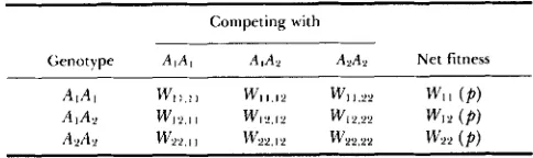
TABLE 3

Genotypic viabilities in pairwise association or competition

Competing with

Genotype A I A , AlA2 AnAn Net fitness

AIAI W I I I , w 1 1 . 1 2 w11.22 WII ( P )

AIAY U'l2.11 WI.L.12 w12.22 W12(Pl

A2A2 W22,Il w 2 2 . 1 2 w2,;22 w 2 2 ( P )

classical selection model. A similar approach is used in our analysis of the frequency-dependent models below.

PAIRWISE INTERACTION MODEL

Consider now the general class of frequency-dependent selection models in which genotypic fitnesses are based on pairwise interactions between the various individuals in the population (e.g., HUANG, SINCH and

KOJIMA 1971; COCKERHAM et al. 1972). Under this

selection scheme the net fitness of an AiAj individual is the weighted average of its fitness taken across all pairwise associations, with

W,,(P) = p2w1,,,,

+

2/41

-

p)wI1.12

+

(1

-

P)'WI 1.22

W1z(p) = p2w12,11

+

2p(1

-

p)w12,12

+

(1

-

p)2w12.22

WZZ(P) = p2w22.11

+

2p(1

-

p ) w 2 2 , 1 2

+

( 1

-

p ) 2 w 2 2 . 2 2 (8)

where in the present notation,

w,,&

(Table 3) is the (constant) viability of genotype A,A, in the presence of genotype ALA,. Since the gene frequency dynamics in (1) are unchanged if the pairwise fitness parameters

Wlj,h, are each multiplied (or divided) by the same

constant factor, we assume without loss of generality that the fitnesses are normalized so that each W,,h, lies in [0, 11.

Note that the pairwise interaction model includes the classical selection model as a special case, since if fitnesses are independent of interactions ( i e . , for each genotype AIA,, W G , ~ , E W, for k, 1 = 1, 2, where WG is

a constant) the net fitnesses reduce to W,(p) = W,. T h e fitness scheme in (8) also subsumes cases of negative frequency dependence. For example, taking W.. 9.4 .. = W,j( 1

-

sg) and W9,k, = W,j for k, I # i, j where

0 <: sg G 1, leads to the net fitnesses Wll(p) =

W11(1

-

s ~ l p ~ ) ,

w , ~ ( p )

= Wl2[1

-

2512p(l

-

p ) ] ,

and W Z ~ (

p )

= Wp,[ 1

-

s22( 1

-

p)'], each of which is a decreasing function of the corresponding genotypic frequency. T h e same example with sij replaced by -sg

(4)

218 M. A. Asmussen and E. Basnayake

TABLE 4

Standard equilibrium patterns for the pairwise interaction model

No. o f polynlorphic equilibria

Equilibrium stability pattern”

0

su

us

1

sus

usu

2

susu

usus

3

susus

ususu

a The end entries indicate the stability of p^ = 0 and p^ = 1 (U = unstable, S = locally stable), while the intermediate entries (if any) refer to the stability of polymorphic equilibria.

Applying the general equilibrium analysis to the pairwise interaction model (8), we find that the internal equilibria are here roots of a complicated cubic equation (APPENDIX B). It is therefore possible to have either 0 , 1, 2, or 3 distinct, polymorphic equilibria in ( 0 , 1). Although the exact number is still difficult to predict in general, some additive X dominance or dominance X dominance effects are necessary for the existence of multiple internal equilibria (COCKERHAM

et al. 1972). T h e derivatives comprising the local stability criterion for polymorphic equilibria (Table 1 ) are complex and can be found in APPENDIX B. T h e local stability criterion for the fixation states (Table

1) are quite simple for this model, however, with

p^

= 0 locally stable whenever W 1 2 , 2 2

<

W 2 2 . 2 2 and

p^

= 1 locally stable whenever W12,11

<

W1l,ll. In or-

der to have a “protected polymorphism” in which neither allele can be lost, it is thus sufficient that each homozygote have a lower fitness in the presence of its own genotype than do heterozygotes in the presence of that homozygote. More precise, necessary and sufficient conditions can be found in COCKERHAM et al. ( 1 972). As we shall see later, however, protected polymorphism conditions greatly underestimate this model’s potential for the maintenance of genetic variation.

T h e complexity of the frequency-dependent fitnesses in (8) precludes a full analytic characterization of the gene frequency dynamics through time. Even the equilibrium structure is complex and difficult to predict, with eight standard equilibrium patterns theoretically possible, in which stable and unstable states alternate along the line from

p

= 0 to

p

= 1 (Table

4). Many other, nonstandard patterns could conceiv- ably arise, however, including ones in which none of the equilibria are stable, if damped or permanent gene frequency oscillations occur. [See MAY (1974) and ASMUSSEN ( 1 986) for ecological and ecological genetic examples of the latter situation.]

Note that again our classification extends to the

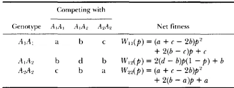
TABLE 5

Pairwise fitnesses under the symmetric model

Competing with

Genotype A , A , A I A y A 2 A 2 Net fitness

A I A , a b c W , , ( p ) = (a

+

c - 2b)p‘

+

2 ( b - c ) p

+

c

AIA? b d b M / 1 2 ( p ) = 2 ( d - b ) p ( l - p )

+

b AYA2 c b a \V,,(p) = (a

+

c - 2 b ) p 2

+

2 ( b

-

a l p

+

a

complete equilibrium set (compare Table 2), including both fixation and (any) polymorphic equilibria. T h e notation in Table 4 therefore differs from that in COCKERHAM et al. (1 972) in that the end entries always denote the stability of

p^

= 0 and

p^

= 1, and the intermediate entries focus simply on the distinct internal equilibria. Their original analysis of a subclass of general dominance models suggests that all the standard patterns shown for polymorphic equilibria can indeed be realized, but gives no indication of their relative frequency in the fitness space nor of the likelihood of convergence to a polymorphic equilibrium.

Greater insight into the potential for genetic polymorphism under the pairwise interaction model is obtained in the next sections through a complete analytic investigation of a new, symmetric version. This analytic study is augmented by an extensive numerical analysis of the symmetric model, the general dominance model of COCKERHAM et al. (1972), and other special cases of particular biological interest, in addition to the general case (Table 3). Together the results help determine when and how often the various equilibrium patterns arise, together with the likelihood of permanent genetic variation under frequency-dependent selection generated by pairwise interactions.

SYMMETRIC PAIRWISE INTERACTION MODEL

We introduce here a symmetric model in which the pairwise fitnesses are principally determined by the degree of genetic similarity of the individuals involved (Table 5). This formulation has some empirical justi- fication (e.g., H U A N G , SINGH and KOJIMA 197 1) and is reminiscent of the classical two-locus symmetric viability model in which fitnesses are based on the genotype’s heterozygosity (see e.g., KARLIN 1975). T h e nine pairwise fitness parameters in the general case (Table 3) are here reduced to four, reflecting the following classes of interactions: homozygote x like- homozygote (a), homozygote X heterozygote ( b ) , homozygote X unlike-homozygote (c), and heterozygote

(5)

Frequency-Dependent Selection 219

like X like interactions between homozygotes and heterozygotes.

The potential internal equilibria are easily derived from the general equilibrium equation (Bl), which here reduces to

( 2 p

-

1)[(4b - u

-

2d

-

c)p(l

-

p )

+

u

-

b] = 0. (9)

Clearly

p^

=

M

is always a solution of (9). Further inspection reveals that the symmetric model has either a single polymorphic equilibrium

(p^

= Y2) or three

polymorphic equilibria (0

<

p^,

<

p^2 = !h

<

p^3

<

l ) , where

c

+

2d

-

3a

PI,

p s = - ₂

-

₂ _a

₊

_2d

+

c

-

4 b ' (10) Three internal solutions arise if and only if b

<

a

<

(c

+

2 d ) / 3 or b

>

a

>

(c

+

2 d ) / 3 , in which case the two outer polymorphic equilibria, p ^ 1 and $3, are sym- metrically located about the central equilibrium $2 =

Yz. Observe from Table 5 that these existence conditions (for multiple internal equilibria) are equivalent to the requirement that the homozygote X like-homozygote fitness ( a ) be intermediate between the homozygote X heterozygote fitness ( b ) , and a weighted average of homozygote x unlike-homozygote (c) and heterozygote x heterozygote fitnesses (d ), in which the latter interactions are given double weight.

Proceeding to the stability analysis, we find that the general local stability conditions in Table 1 and

APPENDIX B here reduce to (i) b

<

a for both

p^

=

0 and

p^

= 1; (ii) a

<

(c

+

2 d ) / 3 for

p^

= !h; and (iii) ( c

+

2 d ) / 3

<

a

<

b for both and $3. Note that the outlying internal equilibria, and $3, are either both locally stable or both locally unstable, whenever they exist. Moreover, the equilibrium structure of the symmetric model depends solely on the relative magnitudes of the three quantities a , b , and ( c

+

2 d ) / 3 , with only four distinct equilibrium patterns possible (Table 6), corresponding to the standard patterns expected with either one or three polymorphic equilibria.

In addition to allowing a complete equilibrium analysis, the prevailing symmetry makes this model, like the classical model, one of the few nonlinear systems for which a complete analytic characterization can be made of the qualitative gene frequency trajectory through time. T h e full behavior is derived in

APPENDIX C and summarized in Table 6. Three im-

mediate observations from this detailed analysis are that, paralleling the classical model, (i) the gene frequency always converges monotonically to a locally stable equilibrium, with no overshooting possible; (ii) the range of initial frequencies (domain of attraction) leading to a locally stable fixation equilibrium ($ = 0 or

p^

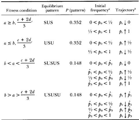
= 1) extends to the nearest unstable (polymorphic) equilibrium; and (iii) the domain of attraction of

TABLE 6

Equilibrium patterns and dynamical behavior under the symmetric model

Equilibrium Initial

Fitness condition pattern P (pattern) frequency" Trajectoryh

(I 2 b,-

c

+

2 d c

3 sus 0.352 0 < P o < % J 0

% < po < 1 p , f 1

(I 5 b,-

c

+

?d<

usu

3 0.352 0 < P o < '/z Pt f YZ

Yz < p , , < 1 p , 1 Y?

b < ( I < - c

+

2d SUSUS 0.148 0 < P O < p ^ ~ p , J 0 3

pl < po < Y2 p , f Yz

p , < PI) < 1 p i

t

1

'!2

< PI, <

j,

pt

.1

%

b > ( I > - c

+

2d USUSU 0.148 0 <PI, < p ^ l p , $1

3

j I <PI, <

'!2

p ,

.1

_SI y Z < p o < p , p t f @

p , <PI, < 1 _{p ,}

₁

_{p 3}

* p^,,

p^,

are defined in Equation 10. ' With at least one inequality strict.

f (1) denotes a monotonically increasing (decreasing) sequence.

a given locally stable polymorphic equilibrium extends to the nearest unstable equilibrium on either side.

Further key observations are evident from the pattern probabilities shown in Table 6. These are derived analytically in APPENDIX D assuming, in analogy to the

classical model above, that the four fitness parameters (Table 5) are independent and uniformly distributed on [0, 11. From the pattern frequencies we conclude that the symmetric model has the potential to produce

(i) three internal equilibria (SUSUS, USUSU) 30% of the time; (ii) two stable internal equilibria (USUSU)

15% of the time; and (iii) one stable internal equilibrium (USU, SUSUS) 50% of the time. This is in strong contrast to the classical model (Table 2 ) for which the corresponding percentages are O,O, and 3 3 .

Even more importantly, there is at least one stable polymorphic equilibrium as long as the homozygote

X like-homozygote fitness ( a ) is less than either the homozygote X heterozygote fitness ( b ) or the weighted average, (c

+

2 d ) / 3 , of the homozygote X unlike- homozygote and heterozygote X heterozygote fitnesses. This means that genetic variation can be preserved under 65% of the symmetric pairwise fitness space, which is almost double the corresponding fraction for the classical selection model. Furthermore, permanent genetic diversity is guaranteed in 50% of the fitness space, since the gene frequency necessarily converges to a polymorphic equilibrium if the homozygote X like-homozygote fitness is less that in homozygote X heterozygote interactions (ie., a

<

b ) .

(6)

220 M . A. Asmussen and E. Basnayake

enhance the likelihood of permanent genetic variation. They also suggest that the simple protected polymorphism condition ( a

<

b ) may seriously underestimate the potential for permanent genetic diversity i n this system. In particular, although both alleles are always maintained by the fitness sets producing a protected polymorphism (USU, USUSU), these underestimate by 23% the fitness sets under which a permanent genetic polymorphism is possible (50% us. 65%).

Similar results hold for the fully symmetric model i n which fitnesses are completely determined by the degree of genetic similarity of the interacting individ-

uals (i.e., d = a ) . In this case the equilibrium structure and dynamical behavior simply depend on the relative magnitudes of the three pairwise fitnesses corresponding to like X like ( a ) , homozygote x heterozygote (b), and homozygote X unlike-homozygote ( c ) interactions. Many of the results above consequently have a more straightforward interpretation, because all conditions involving the weighted average, ( c

+

2 d ) / 3 , reduce to equivalent conditions on the single fitness, c . The quantitative statements are only slightly altered by the change in the pattern probabilities in Table 6 to 1/3, 1/3, 1/6, and 1/6.

The analytic investigation of the symmetric models

demonstrates that frequency-dependent selection

based on pairwise interactions can significantly facilitate the maintenance of genetic variation (relative to the classical, constant fitness regime). The equilibrium pattern probabilities on which these comparisons have been made, however, do not fully measure the potential for permanent genetic variation in frequency- dependent systems, due to the uncertain outcome under patterns where fixation and polymorphic equilibria are simultaneously stable (e.g., SUSUS). In such cases, not all gene frequency trajectories will converge to the stable polymorphic value, since under some initial frequencies the trajectory will converge to 0 or 1. Thus, in contrast to the classical model, the existence of a locally stable polymorphic equilibrium does not generally guarantee that genetic variation will be maintained in the population.

T o properly ascertain the potential for the maintenance of genetic variation under frequency-dependent models, and others where boundary and internal equilibria can be simultaneously stable, we must also compute the average proportion of initial gene frequencies that lead to a polymorphic equilibrium. These expected values are difficult to determine analytically, for even in the fully symmetric case the delimiting frequencies, p ^ l and p^s, defined in (10) have complex functional forms. T h e following sections formally address this issue through an extensive numerical investigation of symmetric and other special forms

of pairwise interactions, as well as of the general case in Table 3 .

NUMERICAL S T U D Y

Twelve different pairwise fitness schemes were analyzed numerically. These include

1. General pairwise interaction model: All 9 pairwise fitnesses (Table 3 ) are independently generated by a random number generator with a uniform distribution on [0, 11.

2. Symmetric pairwise interaction models: T h e four fitness parameters (Table 5 ) are randomly generated from [0, 11, or just three in the fully symmetric case with d = a .

3. General dominance model (COCKERHAM et al. 1972): The dominance parameters, h and k , and the four homozygote X homozygote fitnesses (Wl1,,] for i,

j = 1,

2 )

are randomly generated from [0, 11 and the

remaining fitnesses computed by

W,j,12 = (1

-

k)W,,ll

+

k W i p i , j = 1, 2

and

W1e.ii = (1

-

h ) W l I , ,

+

hW22,ij i , j = 1, 2.

4 . Negatively ordered model (generalization of negative frequency dependence, where individuals are least fit when interacting with others of the same genotype): All 9 pairwise fitnesses (Table 3 ) are randomly generated from [0, 11 and rearranged, if necessary, so that for each genotype AiA,

W . . 11.Y . .

<

wlj,k, for k , 1 # i , j .

5. Fully negatively ordered model (negatively ordered fitnesses where additionally each homozygote’s pairwise fitnesses decrease with increasing genetic similarity of the interacting individuals): All 9 pairwise fitnesses (Table 3 ) are randomly generated from [0, 11 and rearranged, if necessary, so that

W,,,,,

<

W,,,12

<

Wlla i , j = 1, 2 with i # j ,

and

Wl2,ln

<

W I ~ , ~ ~ i = 1, 2.

6. Positively ordered model (generalization of positive frequency dependence where individuals are most fit when interacting with others of the same genotype): All 9 pairwise fitnesses (Table 3 ) are randomly generated from [0, 11 and rearranged, if necessary, SO

that for each genotype AiA,

Wq,,l

>

W,,,, for k , 1 # i , j .

7. Fixed maximum interaction models (where a given genotypic interaction has maximum fitness): One pairwise fitness (wl],kl) is fixed at 1 and the remaining 8 fitnesses are randomly generated from [O, 11.

(7)

Frequency-Dependent Selection 22 1

ness parameters (Wq,hl) were produced by the uniform random number generator (UNIFORM) proposed by

L'ECUYER (1988) for 32-bit computers. This algo-

rithm was selected because of its high periodicity (2.30584 X lo'*)), uniformity, and randomness. We independently verified the latter two properties by a series of four basic tests (APPENDIX E). Two to five

replicate runs, each with at least 20,000 fitness sets (with a maximum of 80,000), were analyzed for each model.

Each fitness scheme was investigated through the four-step procedure outlined below. (Verification of the numerical protocol can be found in APPENDIX E.)

Step 1. Iterate to assess likelihood of genetic variation :

This step was used to identify stable equilibria, the extent of the domains of attraction of all internal equilibria, and any limit cycles or nonmonotonic trajectories. Recursion (1) is iterated from

p~

= 0.01,

. . .

, 0.99 (or in the symmetric cases

PO

= 1/99,

. . .

, 98/99) until convergence

( I

Apt

I

<

lo-') or 10,000 generations, whichever comes first. If

( p , ]

converges for a given

po,

the final iterate is saved as a stable equilibrium value

( j ) ,

and counters updated for (i) the number of sequences (i.e., initial P o values) that converged to a polymorphic equilibrium; and (ii) the number of distinct, stable polymorphic equilibria found for that fitness set. Although iteration cannot locate unstable internal equilibria, a fixation equilibrium is considered unstable at the end of this step if no sequences converged to it. In order to detect the potential for limit cycles and nonmonotonic trajectories, a fitness set is stored for individual investigation and an error signaled if, for any initial

PO,

convergence is not attained in 10,000 generations or the sign of Apt changes at any iterate.

Paralleling other iterative studies (e.g., CLARK and FELDMAN 1986) this step rests on the following prac- tical principle: Two limiting values,

j ,

and

j j ,

are considered equivalent if

I

j,

-

j j

1 <

This as-

sumption further implies that any value less than 1 0-4 is treated as 0, any value greater than 0.9999 is treated as 1, and any value in [O.OOOl, 0.99991 is classified as polymorphic. While this convention may fail to distin- guish between nearby, distinct equilibria, the risk is apparently small, since no nonstandard equilibrium patterns ( i . e . , not in Table 4) were detected.

Step 2. Identijy the equilibrium pattern f o r thejtness set: This step was used to identify all equilibria, both stable and unstable, and as a by-product provided an independent check of whether all stable equilibria were found by iteration. T h e internal equilibria are obtained by first finding all real-valued solutions of the equilibrium equation (Bl) via the cubic-equation- solving-method presented in PRESS et al. (1 986). Roots classified as polymorphic by the convention outlined in Step 1 are then substituted back into ( B l ) and

judged valid if the absolute value of (Bl) is less than lo-'. (This test was always satisfied in our runs.)

The stability of the equilibria are then determined by evaluating (Al) at

j

= 0 and

j

= 1, and (A2) at all internal equilibria, where in deference to possible roundoff error an equilibrium is considered neutrally stable if 1 s I f '(

j )

I

<

1 .OOO 1. Neutrally stable points are then reclassified as stable if they were identified as stable equilibria in Step 1, and otherwise recorded as unstable.

The results are then compared to those from Step 1 with respect to the number of stable polymorphic equilibria, the values of the stable polymorphic equilibria (for agreement to within 1 0-4), and the stability of the fixation states, 0 and 1. In cases where a boundary equilibrium is judged stable by ( A l ) but unstable by Step 1 (e.g.,

I

f '(0)

I

<

1 but no trajectories converged to

p

= 0) the program attempts to resolve the discrepancy by performing an additional iteration from

po

= 0.0001 for

p

= 0, or P o = 0.9999 for

p =

1.

If there is no discrepancy, the equilibrium pattern is classified and the following 19 statistics updated: (1-3) N t : the number of fitness sets with i = 1, 2, or 3 distinct, polymorphic equilibria; (4-6) Nip: the number of initial frequencies that converge to a polymorphic equilibrium, for those fitness sets with exactly i = 1, 2, or 3 stable polymorphic equilibria; (7-14) Num-pattern: total number of fitness sets with the observed equilibrium pattern (pattern) found in Table 4; (15-18) P-pattern: total number of initial frequencies that converge to a polymorphic equilibrium, if the equilibrium pattern (pattern) is USU, SUSU,

USUS, or SUSUS; and (19) FITSETS: the number of

fitness sets with no errors.

A fitness set is stored for individual investigation and an error signaled if either the results from the two steps disagree or the observed pattern is not shown in Table 4.

Step 3. Calculate measures of genetic variation : After each 10,000 fitness sets the following 20 probability statistics are calculated, based on the cumulative error free fitness sets (where n = total number of initial frequencies used for iterating each fitness set): (1 -8)

P(pattern) = (Num-pattern)/FITSETS, for each equilibrium pattern in Table 4; (9-1 1) P(exact1y i stable polymorphic equilibria) = NJFITSETS, for i = 1, 2, and 3; (1 2-14) P(converge to a polymorphic equilibrium given there are i stable internal equilibria) = Nip/

[Ni

X n ] , for i = 1,

2,

and 3; (15) P(converge to a polymorphic equilibrium) =

x:=,

Nip/[FITSETS X n];

(16) P(protected polymorphism) = P(USU)

+

P(USUSU); and (1 7-20) P(converge to a polymorphic

equilibrium given the equilibrium pattern) =

(8)

222 M. A. Asmussen a n d E. Basnayake

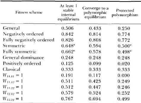
TABLE 7

Summary probabilities for pairwise interaction models

0.506 0.433 0.250

0.842 0.814 0.774

0.648" 0.594 0.500"

0.662" 0.578 0.498"

0.248 0.248 0.248

0.125 0.099 0.020

0.333 0.333 0.333

0.191 0.117 0.000

0.5 1 1 0.423 0.249

0.512 0.447 0.246

0.579 0.524 0.252

0.767 0.694 0.499

Wd 0.826 0.808 0.772

" N o t ? close agreement to analytic values in Table 6 and text.

terns with exactly one stable polymorphic equilibrium (i.e., USU, SUSU, USUS, SUSUS).

A model's run is terminated after 100,000 fitness sets, or if the following 14 statistics agree to within

5 X of their values after the last 10,000 sets: the probabilities in (1 -8) corresponding to patterns with exactly one stable polymorphic equilibrium, and all probabilities in (9-14) and (17-20).

Step 4 . Individually examine all fitness sets which sig- nal errors: All fitness sets/limiting values saved because of nonmonotonic trajectories, nonconvergence after 10,000 generations, a discrepancy between steps

1 and 2, or a nonstandard equilibrium pattern are individually investigated with the aid of a special program which implements Steps 1-3. N o more than 109 (with an average of 20) of the 20,000-80,000 fitness sets on a run fell in this category.

Numerical results: T h e numerical results are summarized in Tables 7-9, where in each case the values shown represent the average across 2 to 5 replicate runs. Key features of this analysis are highlighted below.

1. Probability of at least one stable internal equilib- rium: The summary statistics in Table 7 confirm that genotypic interactions can greatly facilitate the maintenance of genetic variation. In the general model 5 1% of the pairwise fitness space produces at least one stable polymorphic equilibrium as opposed to 33% of the fitness space for the classical model and 65-66% of the fitness space for the symmetric models. This probability has a remarkable maximum of 84% in the negatively ordered model, where individuals are least fit when interacting with another of their own genotype. Interestingly, this value is slightly lower (83%) in the fully negatively ordered case, where additionally each homozygote's pairwise fitnesses decrease with increasing genetic similarity of the interacting

individuals. In contrast, a stable polymorphic equilibrium exists for only 25% of the general dominance fitnesses (COCKERHAM et al. 1972), and, in keeping with the analytical results for the symmetric model (Table 6), is least likely (1 3%) in the positively ordered case.

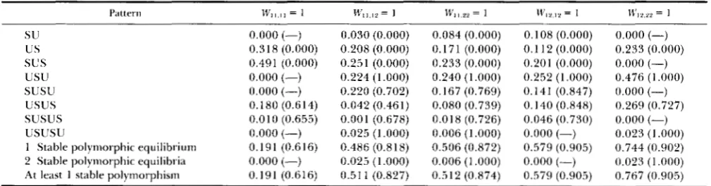
The fixed maximum interaction models provide further insight into the types of interactions which increase or decrease the likelihood of a stable polymorphic equilibrium. On average, this likelihood is

lowest (19%) when a homozygote X like-homozygote

interaction fitness is highest (W, = l), and greatest (77%) when a heterozygote x homozygote fitness is highest (W12.22 = 1). T h e two extreme values thus

correspond to the two fitness schemes which respectively insure the stability or instability of one of the fixation states (see Table 1). In the other three cases, where a homozygote x heterozygote fitness is maximal ( W I I , I ~ = l ) , a homozygote X unlike-homozygote fitness is maximal (W11.22 = l ) , o r the heterozygote x

heterozygote fitness is maximal (W12.12 = 1) the boundary equilibria may be either stable or unstable. For the first two of these, the likelihood of a stable polymorphic equilibrium is equivalent to that for the general model (5 1 %), and interestingly is only slightly higher (58%) in the third ( W 1 2 , , 2 = l ) , which could be viewed as the heterotic, pairwise fitness scheme.

2. Probability of converging to a polymorphic equilib- rium: A more precise measure of the potential for permanent genetic variation is provided by the overall fraction of initial gene frequencies which lead to a polymorphic equilibrium. This statistic exhibits the same relative ordering as the probability of having at least one stable internal equilibrium, and is in fact only slightly reduced by the possible simultaneous stability of one or both fixation equilibria. For the basic models in Table

7

(i.e., not fixed-maximum), the probability of converging to a polymorphic equilibrium is again only less than the classical value (33%) in the general dominance (25%) and positively ordered (1 0%) models. On average, a polymorphic equilibrium is reached for 43% of the fitness space/initial frequencies in the general case and for 81 % in the negatively ordered models. This value is intermediate (58-59%) for the symmetric models.

In the fixed maximum interaction models, the likelihood of converging to an internal equilibrium

ranged from a minimum average value of 12% when a homozygote x like-homozygote fitness is highest ( W l l , l l = I), to a maximum average value of 69% when a heterozygote x homozygote fitness is highest (W,2,22 = 1). In the other three cases, this probability is similar to that in the general model (43%), with a notable difference only in the heterotic scheme ( W 1 2 . 1 2 = 1) where the value is increased to 52%.

(9)

TABLE 8

Pattern and conditional convergence probabilities

Pattern General _{ordered" dominance} ~ y r n m e t r i c ~ General Positively _ordered Classiral

su

0.127 (0,000) 0.074 (0,000) 0.000 (-) 0.251 (0,000) 0.057 (0,000) 0.167 (0.000)

C S 0.128 (0.000) 0.063 (0.000) 0.000 (-) 0.253 (0.000) 0.084 (0.000) 0.167 (0.000)

sus

0.239 (0.000) 0.020 (0.000) 0.352 (0.000) 0.247 (0.000) 0.734 (0.000) 0.333 (0.000)

usu

0.238 (1.000) 0.736 (1.000) 0.352 (1.000) 0.248 (1.000) 0.020 (1.000) 0.333 (1.000)

susu

0.124 (0.718) 0.039 (0.585) 0.000 (-) 0.000 (-) 0.022 (0.817) 0.000 (-)

usus

0.120 (0.715) 0.029 (0.582) 0.000 (-) 0.000 (-) 0.046 (0.800) 0.000 (-)

SUSUS 0.013 (0.712) 0.000' (-) 0.147 (0.632) 0.000 (-) 0.037 (0.656) 0.000 (-)

ususu

0.012 (1,000) 0.038 (1.000) 0.148 (1.000) 0.000 (-) 0.000' (-) 0.000 (-)

1 Stable polymorphic equilibrium 0.494 (0.853) 0.804 (0.965) 0.499 (0.891) 0.248 (1.000) 0.125 (0.792) 0.333 (1.000)

2 Stable polymorphic equilibria 0.012 (1.000) 0.038 (1.000) 0.148 (1.000) 0.000 (-) 0.000'(-) 0.000 (-)

At least 1 stable polymorphism 0.506 (0.856) 0.842 (0.967) 0.648 (0.916) 0.248 (1,000) 0.125 (0.792) 0.333 (1.000)

Pattern probabilities followed by P(converge to polymorphic equilibrium I pattern) in parentheses for each pattern with frequency of a t

" For the fully negatively ordered model, the pattern probabilities are within 0.03 of the entries for the negatively ordered model; the

For the fully symmetric model, the pattern probabilities are within 0.03 of those for the symmetric model; the conditional conver-gence

Pattern occurred i n only 1-2 fitness sets, with frequency of 5 X 10" or less. lKlst 5 X

conditional convergence probabilities differ only for SUSU (0.667), USUS (0.659), and for 1 and at least 1 stable polymorphism (0.978).

probabilities differ only for SUSUS (0.492) and for 1 stable (0.830) and at least 1 stable (0.874) polymorphism.

TABLE 9

Pattern and conditional convergence probabilities for the fixed maximum interaction models

Pattern

w,,,,,

= 1 n.,,.,, = 1 LV,,,,, = 1 w,,,,, = 1 12'1,,,, = 1

SU 0.000 (-) 0.030 (0,000) 0.084 (0,000) 0.108 (0.000) 0.000 (-)

us

0.318 (0.000) 0.208 (0.000) 0.171 (0.000) 0.1 12 (0.000) 0.233 (0.000)

sus

0.491 (0.000) 0.251 (0,000) 0.233 (0.000) 0.201 (0.000) 0.000 (-)

usu

0.000 (-) 0.224 (1.000) 0.240 (1.000) 0.252 (1.000) 0.476 (1.000)

SUSU 0.000 (-) 0.220 (0.702) 0.167 (0.769) 0.141 (0.847) 0.000 (-)

usus

0.180 (0.614) 0.042 (0.461) 0.080 (0.739) 0.140 (0.848) 0.269 (0.727)

SUSUS _{0.010 (0.655)} _{0.001 (0.678)} _{0.018 (0.726)} _{0.046 (0.730)} _0.000_(-)

USUSU _0.000_(-) _{0.025 (1.000)} _{0.006 (1.000)} _0.000_(-) _0.023_{( I}_,000)

1 Stable polymorphic equilibrium _{0.191 (0.616)} _{0.486 (0.818)} _{0.506 (0.872)} _{0.579 (0.905)} _{0.744 (0,902)}

2 Stable polynlorphic equilibria _0.000_(-) _{0.025 (1}_.OOO) _{0.006 (1}_.000) _0.000_(-) _{0.023 (1.000)}

At least 1 stable polymorphism _{0.191 (0.616)} _0.51₁_(0.827) _{0.512 (0.874)} _{0.579 (0.905)} _{0.767 (0,905)}

Pattern probabilities followed by P(converge to a polymorphic equilibrium I pattern) for each pattern with frequency of at least 5 X 10".

mate of the potential for permanent genetic variation: It is clear from Table

7

that the probability of a protected polymorphism ( i . e . ,

p^

= 0 and

p^

= 1 both unstable) is usually a poor estimate of the full potential for permanent genetic variation. For the general

model this probability underestimates the likelihood of having a stable internal equilibrium by 51 %, and the probability of actually converging to a polymorphic equilibrium by 42%. T h e same is true for the three middle fixed maximum models in which a homozygote x unlike-type or heterozygote x heterozygote fitness is maximal. T h e discrepancies are some- what less in the other special cases, with the exception of the two fitness schemes with the lowest potential for permanent genetic variation. For the positively ordered model, the protected polymorphism condition underestimates the more precise measures of genetic variation by 5- to 6-fold. T h e worst discrepancy occurs under the fixed maximum interaction model where a homozygote X like-homozygote fitness

is maximal ( W I I , l l = 1). In this case there is never a protected polymorphism, yet there is a stable internal equilibrium 19% of the time and one is reached 12% of the time. Interestingly, the protected polymorphism conditions appear to be perfect predictors of the maintenance of genetic variation in the general dominance model just as in the classical model (see pattern probability discussion below).

(10)

224 M. A. Asmussen and E. Basnayake

imal. At the opposite extreme, only four patterns were found for the classical, general dominance, and symmetric models, as well as for the fixed maxilnum models where a homozygote X like-homozygote or heterozygote X homozygote fitness is maximal. (iii) For some models, the missing patterns may be corn- pletely excluded by the fitness regime. Such is the case for the classical model, the symmetric models, and the fixed maximum models in which Wti.lt = 1 or

1 1 1 1 2 , ~ ~ = 1 for i = 1 or 2. In other models, the missing

patterns lTlay be theoretically possible but restricted

to such a small range of their fitness space that they were not encountered. This seems the most likely explanation of the results for the general dominance model, since although its stability analysis (COCKER-

HAM et al. 1972) appears to have been based on an analog of the insufficient condition,f’( p^)

<

1, rather than the full stability criterion in (6), the model did not produce any nonmonotonic trajectories (which should occur wheneverf‘(6)

<

O}. (iv) With the slight exception of the general dominance case, the two equilibrium patterns with one internal equilibrium (SUS, USU) are together the most frequent. In the general case these constitute almost half the total distribution, with the twin patterns with zero or two internal equilibria each occurring in 24-25% of the fitness space, and the two patterns with three internal equilibria occurring in less than 3% of the fitness space. (Note the symmetric frequencies for each pair of patterns with the same number of internal equilibria.) (v) Although it is possible to have t w o stable polymorphic equilibria, this evidently only occurs in a small subset of the total fitness space. The associated pattern (USUSU) was only produced by -1% of the general pairwise interaction fitness space and by less than 4% of the fitness space for all the special cases except the t w o bymmetric models. I t was never encountered in the general dominance model or in the fixed maximum models where a like X like fitness is maximal, and occurred only twice in the positively ordered model. Note that the latter findings are consistent with the analytic results for the symmetric model (Table 6). (vi) Each pattern probability obtained under the negatively ordered model is close to that for the “complementary” pattern (i.e., the pattern obtained by replacing every “ U ” by “S” and every “S” by “ U ” ) in the positively ordered model.

5. Probability of Converging to a polymorphic equilib- rium given the equilibrium pattern: T h e conditional probabilities in Tables 8 and 9 show that genetic variation is very likely to be maintained in all cases where there is a stable polymorphic equilibrium (USU, SUSU, USUS, SUSUS, USUSU). In the general model, the gene frequency converges to a polymorphic value 86% of the time that a t least one stable polymorphic equilibrium exists. Although this always

occurs when both fixation states are unstable (USU, USUSU), a stable polymorphic equilibrium is even reached (on average) from over 7 1% of the initial frequencies when one or both fixation states are also stable.

T h e various special models are also very apt to maintain both alleles whenever there is at least one stable polymorphic equilibrium. T h e likelihood is lowest, but still fairly high (62%), for the fixed maximum model where a homozygote X like-homozygote fitness is maximal, and highest (97%) for the negatively ordered model. The values in the other cases range from 79 to 92%. With a single exception (USUS pattern when W,,,12 = 1) the probability of converging to a polymorphic value exceeds, and often greatly so, the fraction of stable equilibria that are polymorphic. (The classical and general dominance models are omitted from this discussion because both fixation states are, or were found to be, unstable whenever a stable internal equilibrium exists.) T h e surprisingly high probabilities of converging to a stable polymorphic equilibrium in the presence of one or more stable fixation equilibria (ie., for SUSU, USUS, and SUSUS patterns) further account for the generally high likelihood of maintaining genetic variation in the pairwise interaction model, as well as for the often poor performance of protected polymorphism conditions as a measure of this potential.

6. Nonmonotonic trajectoriesllimit cycles: In contrast to the symmetric model, fitness sets with nonmonotonic gene frequency trajectories are possible under other pairwise fitness schemes. Such behavior is rare, however, and was found only in runs for the general pairwise interaction model, the negatively ordered model, and the fixed maximum model with a homozygote x unlike-homozygote fitness maximal. In all nonmonotonic trajectories the gene frequency over- shot the ultimate equilibrium in the first generation, with the subsequent trajectory generally converging very quickly, either monotonically or with further oscillations.

Most fitness sets with errors were so identified because of nonconvergence in the allotted 10,000 generations, All such cases were found upon individual investigation to be converging to an equilibrium frequency, albeit very slowly, without any cyclical behavior. Since there is no evidence of limit cycles, the statistics concerning polymorphic equilibria suffice to assess the potential for genetic variation in this class

of models.

DISCUSSION

(11)

tion (e.g., KARLIN and CARMELLI 1975; LEWONTIN,

GINZBURC and TULJAPURKAR 1978; KARLIN 1981;

K A R L I N and FELDMAN 198 1 ; CLARK and FELDMAN

1986). The results from such studies provide a novel perspective on the biological conditions which enhance or reduce this potential, as well as on the relative strengths of their effects. Here, the primary measures of genetic variability are (i) the fraction of pairwise fitness sets which produce at least one stable polymorphic equilibrium; and (ii) the overall fraction of initial gene frequencies, averaged across all possible fitness sets, which converge to an internal equilibrium, calculated under the assumption that the pairwise fitnesses are independently and uniformly distributed on [O, 11.

Our first step involved a complete analytic description of the equilibrium structure and dynamical behavior under a symmetric model, in which the pairwise fitnesses depend on the genetic similarity of the individuals involved. This was supplemented by an extensive numerical investigation of the equilibrium patterns and gene frequency dynamics under the general pairwise interaction model, as well as under the symmetric model and other special cases. A key aspect of the numerical study was an assessment of the com- bined domains of attraction of stable polymorphic equilibria.

T h e results from both phases of the study provide concrete evidence that models which incorporate the frequency-dependent effects of pairwise interactions have a high potential for permanent genetic variation. For general pairwise fitnesses, the probabilities of producing at least one stable internal equilibrium and of actually converging to a polymorphic frequency are respectively 51% and 4396, versus 33% for the classical, constant viability selection model. These probabilities are both highest (84% and 8 1 %) when like

x

unlike interactions are beneficial with respect to those between like types (negatively ordered fitnesses), and lowest (1 3% and 10%) when like X unlike interactions are detrimental (positively ordered fitnesses). In the symmetric models these two conditions respectively insure and preclude the maintenance of genetic variation. T h e potential for permanent genetic variation is only reduced below that in the classical model when each individual’s fitness is highest in association with like genotypes (positively ordered model), a homozygote X like-homozygote fitness is maximal, or fitnesses satisfy the conditions of the general dominance model (COCKERHAM et al. 1972).

These results are consistent with qualitative predic- tions on biological grounds, as well as with theoretical demonstrations of an increased retardation of fixation in finite populations under certain pairwise fitness arrays (HEDRICK 1972, 1973). What is perhaps sur- prising, however, is the actual extent to which inter-

genotypic interactions can enhance or reduce genetic variability. Our quantitative results also provide a number of other useful insights into this class of models. For instance, the numerical analyses of the negative and fully negatively ordered models show that the likelihood of maintaining genetic variation is not increased if in addition to having each genotype’s fitness lowest in association with another of the same genotype, each homozygote’s pairwise fitnesses are decreasing functions of the genetic similarity of the interacting individuals.

Another important point, from the numerical investigation of the set of fixed maximum models, is that it is the homozygote X like-homozygote and heterozygote X homozygote fitnesses which, presum- ably because they determine the stability of the fixation states, have the greatest impact on the likelihood of genetic diversity. Interestingly, the “heterotic” pairwise fitness scheme, in which the heterozygote x heterozygote fitness is maximal, is only slightly more likely to preserve both alleles than is the “average” pairwise fitness scheme. In the same vein, the heterozygote X heterozygote fitness only affects the outcome under the symmetric model as part of a weighted average including the homozygote X unlike-homozygote fitness. Although the stability of the boundary equilibria strongly influences the likelihood of stable polymorphic equilibria and of ultimately converging to a polymorphic frequency, the conditions for a protected polymorphism, which ensure genetic variability through the instability of both fixation states, underestimate by an average of 50% the full potential for permanent genetic variation.

The increased likelihood of maintaining both alleles, and the poor performance of a protected polymorphism as a measure of this likelihood, are caused primarily by a greater variety and frequency of equilibrium patterns with one stable polymorphic equilibrium, in conjunction with a large domain of attraction for stable internal equilibria. For instance, on average, the gene frequency converges to a polymorphic value 86% of the time that a stable internal equilibrium exists, and even does so over 71% of the time if one or both fixation states are simultaneously stable. The existence of multiple, stable internal equilibria, on the other hand, does not contribute significantly to the increased potential for genetic variation in these models since, although it is possible to have two stable internal equilibria, this situation is highly unlikely except in the symmetric models, where it occurs in