Semiparametric Regression Methods for Longitudinal Data with Informative Observation Times and/or Dropout.

ABSTRACT

CAI, NA. Semiparametric Regression Methods for Longitudinal Data with Informative Observation Times and/or Dropout. (Under the direction of Dr. Wenbin Lu and Dr. Hao Helen Zhang.)

Semiparametric Regression Methods for Longitudinal Data with Informative Observation Times and/or Dropout

by Na Cai

A dissertation submitted to the Graduate Faculty of North Carolina State University

in partial fulfillment of the requirements for the Degree of

Doctor of Philosophy

Statistics

Raleigh, North Carolina 2011

APPROVED BY:

Dr. Anastasios A. Tsiatis Dr. Daowen Zhang

Dr. Wenbin Lu

Co-chair of Advisory Committee

DEDICATION

BIOGRAPHY

ACKNOWLEDGEMENTS

This dissertation would not have been possible without the guidance and support from many individuals who contributed their valuable assistance during my graduate study at North Carolina State University.

First and foremost, my deepest thanks and appreciation are given to my advisors, Dr. Wenbin Lu and Dr. Hao Helen Zhang, whose courage, support and extraordinary guidance I will never forget. Without their wise advice and assistance, this work would not have been possible. Dr. Wenbin Lu and Dr. Hao Helen Zhang have always been so understanding and patient whenever I needed. And, I want to thank Dr. Wenbin Lu for the financial assistance which allowed me to complete my Ph.D in statistics. I was extraordinarily fortunate in having them as my advisors.

I would like to thank Dr. Anastasios Tsiatis and Dr. Daowen Zhang for serving on my committee. I am grateful for their time and valuable suggestions on the thesis work. I am also thankful to Dr. David Dickey, Dr. Howard Bondell and Dr. Jason Osborne for their help and courage when I started my PhD study in Statistics. And, thanks Dr. Howard Bondell for the support in my job searching. Moreover, I owe my gratitude to Dr. Zhao-Bang Zeng for his guidance and assistance when I was in bioinformatics program and his understanding when I decided to continue my PhD study in statistics. I would also like to thank all faculty and staff members in statistics department and bioinformatics program for valuable guidance and assistance throughout my graduate study.

TABLE OF CONTENTS

List of Tables . . . viii

List of Figures . . . ix

Chapter 1 Time-Varying Latent Effect Model for Longitudinal Data with Informative Observation Times . . . 1

1.1 Introduction . . . 1

1.2 Existing Methods . . . 4

1.2.1 Semiparametric Regression Model . . . 4

1.2.2 Joint Modeling . . . 6

1.3 Model Specification . . . 7

1.4 Estimation Procedure and Asymptotics . . . 9

1.5 Model Diagnostic . . . 14

1.6 Numerical Studies . . . 16

1.6.1 Simulation Studies . . . 16

1.6.2 Analysis of Bladder Cancer Data . . . 22

1.7 Proofs of Asymptotic Results . . . 26

1.7.1 Consistency of Proposed Estimators . . . 27

1.7.2 Asymptotic Normality of Proposed Estimators . . . 29

Chapter 2 Semiparametric Regression Analysis for Longitudinal Medi-cal Cost Data with Informative Hospitalization and Death . 37 2.1 Introduction . . . 37

2.2 Existing Methods . . . 40

2.2.1 Methods for Lifetime Medical Cost . . . 40

2.2.2 Methods for Longitudinal Medical Cost . . . 42

2.3 Model and Inference . . . 44

2.3.1 Model and Notation . . . 44

2.3.2 Estimation Procedure . . . 46

2.4 Asymptotic Results . . . 49

2.5 Estimation and Inference of Cumulative Medical Cost . . . 54

2.6 Numerical Studies . . . 56

2.6.1 Simulation Studies . . . 56

2.6.2 Analysis of Medical Cost Data . . . 61

2.7 Proofs of Asymptotic Results . . . 67

2.7.2 Asymptotic Properties of Perturbed Estimators for Regression

Co-efficients . . . 75

2.7.3 Asymptotic Properties of Estimated Cumulative Medical Cost . . 79

Chapter 3 Discussion and Future Work . . . 82

3.1 Discussion and Future Work (I) . . . 82

3.2 Discussion and Future Work (II) . . . 84

LIST OF TABLES

Table 1.1 Simulation results based on 500 Monte Carlo replications with sam-ple size equal to 200. Est. is the mean of parameter estimates. SD is the sample standard deviation of parameter estimates. SE is the mean of estimated standard errors. CP is the coverage probability of 95% Wald-type confidence intervals. . . 19 Table 1.2 Analysis results of the bladder cancer data for patients with

super-ficial bladder tumors. Est. is the estimate for parameters. SE is the estimated standard error of parameter estimates. . . 24 Table 2.1 Simulation results based on 500 Monte Carlo replications with

sam-ple size equal to 200. Estimated standard errors are obtained based on 100 resamplings. Est. is the mean of parameter estimates. SD is the sample standard deviation of parameter estimates. SE is the mean of estimated standard errors. CP is the coverage probability of 95% Wald confidence intervals. . . 60 Table 2.2 Analysis of medical cost data for chronic heart failure patients.

LIST OF FIGURES

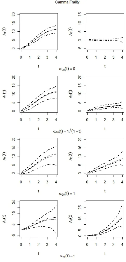
Figure 1.1 Plot of averages of estimated functions for nonparametric functions when the latent variable is a mixture of gamma random variables. The results are based on 500 Monte Carlo replications with sam-ple size equal to 200. Dashed lines are underlying true functions; solid lines are averages of estimated functions; dash-dot lines are pointwise 95% confidence intervals. . . 20 Figure 1.2 Plot of averages of estimated functions for nonparametric functions

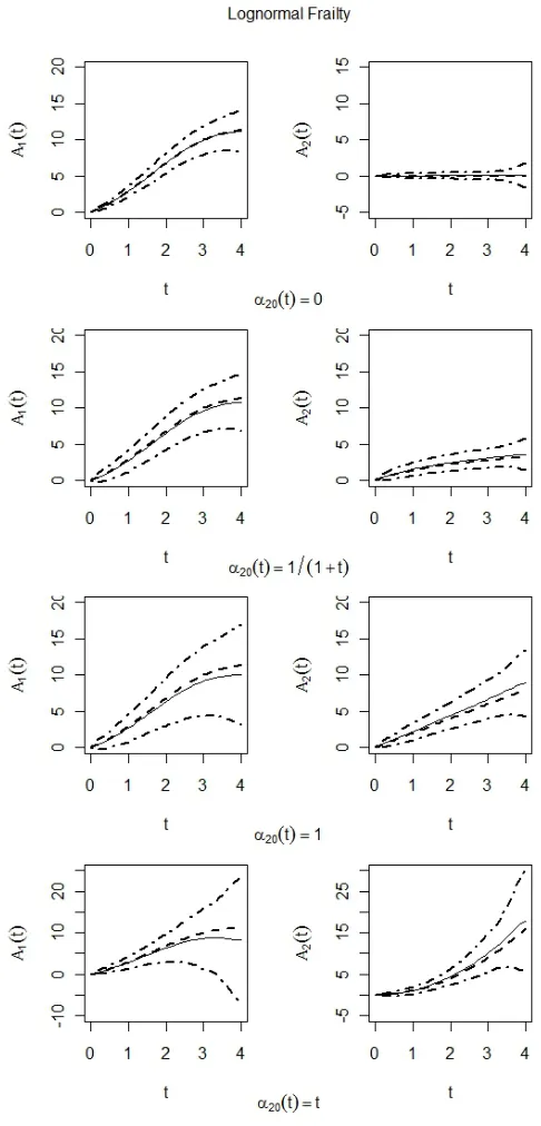
when the latent variable is a mixture of log-normal random vari-ables. The results are based on 500 Monte Carlo replications with sample size equal to 200. Dashed lines are underlying true func-tions; solid lines are averages of estimated funcfunc-tions; dash-dot lines are pointwise 95% confidence intervals. . . 21 Figure 1.3 Plot of the average of estimated functions for the baseline

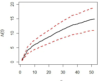
cumu-lative intensity function Λ0(t). The solid line represents the point

estimates of Λ0(t) and dashed lines are corresponding pointwise

95% confidence intervals. . . 25 Figure 1.4 Plot of averages of estimated functions for nonparametric functions

A10(t) and A20(t). The solid lines represent the point estimates

of A10(t) (left panel) and A20(t) (right panel). Dashed lines are

corresponding pointwise 95% confidence intervals. . . 25 Figure 2.1 Estimated mean cumulative medical costs for different groups of

individuals. Corresponding pointwise 95% confidence intervals are constructed based on 100 resamplings. Solid lines are estimated mean cumulative medical costs ; dash lines are corresponding point-wise 95% confidence intervals. . . 64 Figure 2.2 Estimated mean cumulative medical costs for different groups of

individuals. Corresponding pointwise 95% confidence intervals are constructed based on 100 resamplings. Solid lines are estimated mean cumulative medical costs ; dash lines are corresponding point-wise 95% confidence intervals. . . 65 Figure 2.3 Estimated mean cumulative medical costs for different groups of

Chapter 1

Time-Varying Latent Effect Model

for Longitudinal Data with

Informative Observation Times

1.1

Introduction

al., 2009) were developed accordingly. All of these methods assume that the effect of latent variables on longitudinal outcomes is time-invariant, that is, the latent effect does not change over time, which may be restrictive in practice. Since both observation times and outcomes are time-dependent stochastic processes, it is more plausible to assume that the latent variable effect on outcomes changes over time. In the numeric studies, our analysis results on the bladder cancer data suggest that the latent variable effect is truly time-dependent. How to characterize the time-dependent behavior of the latent effect shared by the outcome and observation time processes is of main interest here.

of the tests. In particular, we can formally test whether the latent effect is null or the constant 1, which respectively corresponds to the model assumptions made in Lin and Ying (2001) and Sun et al. (2007). In Section 1.6, we apply our method to the bladder cancer data. Based on the results from our new method, we discover that the effect of the latent variable on longitudinal outcomes is actually time-varying since the proposed goodness-of-fit tests reject the null hypotheses of no effect and constant effect of 1 for the latent variable.

1.2

Existing Methods

As we mentioned in the introduction, various methods have been developed to study longitudinal data in presence of irregular and/or informative observation times. Our method can be considered as a generalization of the semiparametric regression model of Lin and Ying (2001) and the shared random-effect model of Sun et al. (2007). For comparison, more details about the models of Lin and Ying (2001) and Sun et al. (2007) are given in the following.

1.2.1

Semiparametric Regression Model

First, we introduce common notations used in this chapter to describe longitudinal data and observation times. Consider a longitudinal study of n subjects. For the ith subject, letYi(t) be the underlying longitudinal outcome at time t and Xi be the p×1 vector of

baseline covariates. In addition, letTi1 < Ti2 <· · · denote the potential observation times

of longitudinal outcomes andCi denote the follow-up time. LetNi∗(t) =

P∞

j=1I(Tij ≤t)

realizations from the counting process censored at the end of follow up and Yi(t) is only

observed at the jump points of Ni(t). Then, Lin and Ying (2001) proposed the following

semiparametric regression model for the longitudinal outcome Yi(t)

E{Yi(t)|Xi}=α0(t) +β00Xi,

whereα0(t) is an arbitrary function oft, andβ0 is a p×1 vector of regression coefficients.

And, the model for observation times are given as follows

E{dN_i∗(t)|Xi}= exp(γ00Xi)dΛ0(t),

whereγ0is ap×1 vector of regression coefficients and Λ0(t) is an arbitrary nondecreasing

function.

For estimation of parameters, it is assumed that, Ci, Ni∗(·) and Yi(·) are mutually

independent given covariatesXi. Hence, both censoring times and observation times are

assumed to be noninformative to longitudinal outcomes given covariates. Then, under the models and assumption, they defined the following mean-zero process

Mi(t;A, β, γ) =

Z t

0

[{Yi(s)−β0Xi}dNi(s)−I(Ci ≥s)eγ

0_X

i_dA(s)],

where A(t) = Rt

0 α(s)dΛ(s). The following set of estimating equations are proposed to

estimate A0(t) and β0 simultaneously

n

X

i=1

Mi(t;A, β, γ) = 0 n

X

i=1

Z ∞

0

where W(t) is a weight function. It can be shown that estimators for A0(t) and β0 can

be obtained by solving the above estimating equations simultaneously. In addition, they also considered more general models which incorporate time-dependent covariates Xi(t)

with time-varying regression coefficients β0(t). And they proposed an estimator for the

weighted sum of the regression coefficients B0(t) =

Rt

0β0(s)dΛ0(s) instead of β0(t).

1.2.2

Joint Modeling

In the study of Lin and Ying (2001), they assumed independence between longitudinal outcomes and observation times given covariates. In practice, longitudinal outcomes may be correlated with observation times through some unobserved confounders. For example, Sun et al. (2007) proposed a joint model for longitudinal outcomes and observation times. Let Vi be a nonnegative latent variable with E(Vi|Xi) = 1. The distribution of latent

variable is completely unspecified. Given covariates Xi and the latent variable Vi, they

proposed to model the longitudinal outcomeYi(t) as follows

E{Yi(t)|Xi, Vi}=α0(t) +β00Xi+Vi,

which can be considered as an extension of the model of Lin and Ying (2001). Given covariatesXi and the latent variableVi, the conditional intensity of the counting process

N_i∗(t) is modeled as

λ(t|Xi, Vi) =Viλ0(t)exp(γ00Xi).

In the models, the correlation between longitudinal outcomes and observation times is described by the shared latent variable Vi. And the effect of the latent variable on

could be too restrictive. Later, Liang et al. (2009) proposed a joint model with more flexible correlation structures for longitudinal outcomes and observation times. In their model, the association between longitudinal outcomes and observation times is modeled via correlated latent variables. But, for estimation of parameters, they need to specify the distribution of latent variables, which may be too restrictive in practice.

1.3

Model Specification

In these existing methods, the effects of latent variables on longitudinal outcomes are assumed to be time-independent. In our study, we are interested in developing a more flexible joint model which allows time-varying dependence between longitudinal outcomes and observation times. Here, we adopt the same notations for longitudinal outcomes and observation times used in the previous section. And, letmi ≡Ni(∞) be the total number

of observations made on the ith subject. Then, we consider the following time-varying latent effect model for the longitudinal outcome:

E{Yi(t)|Xi, Vi}=α10(t) +Viα20(t) +β00Xi, (1.1)

where α10(t) and α20(t) are unspecified smooth functions of timet, the random effect Vi

is a nonegative latent variable with E(Vi|Xi) = 1 and V ar(Vi) > 0, and β0 is a p×1

vector of unknown regression coefficients. The marginal model (1.1) characterizes the mean of the process Yi(·) only, and does not specify its distribution and the dependence

structure among repeated measurements. Given the covariatesXi and the latent variable

the conditional intensity function given by

λ(t|Xi, Vi) =Viλ0(t) exp(γ00Xi), (1.2)

whereλ0(t) is an unspecified baseline intensity function andγ0 is ap×1 vector of unknown

regression coefficients. Such a multiplicative frailty model has also been considered by other authors for describing the observation time process (e.g. Sun et al., 2007; Liang et al., 2009) as we introduced in the previous section.

Two key features of models (1.1) and (1.2) are: first, the dependence betweenYi(t) and

N_i∗(t) is characterized by a shared latent variableVi; second, Vi has a time-varying effect

on the outcome processYi(t). This time-varying latent effect model is very comprehensive

as it contains many existing models as special cases. For example, when α20(t) ≡ 0,

implying that Yi(·) and Ni∗(·) are independent givenXi, it becomes the marginal model

considered by Lin and Ying (2001); When α20(t)≡ 1, (1.1) becomes the model studied

by Sun et al. (2007) that assumes a positive time-invariant effect of the latent variable. However, eitherα20(t) = 0 or 1 for the effect of the latent variable could be too restrictive

in practical applications, as suggested by our real example analysis. By allowing a time-varying effect of the latent variable, the proposed model provides a more flexible way to describe the complex relationship between Yi(·) andNi∗(·). Throughout this chapter, we

make the following assumptions: (i) Yi(·) is independent of Ni∗(·) given Xi and Vi; (ii)

Ci can depend on Xi in an arbitrary way, but Ci is independent of Yi(·), Ni∗(·) and Vi

givenXi. In models (1.1) and (1.2), the distributions ofVi andCi, the baseline functions

α10(t) and λ0(t), and the time-varying coefficient α20(t) of Vi, are all left unspecified, so

1.4

Estimation Procedure and Asymptotics

Note that model (1.2) is a special case of the proportional mean/rate model since it follows that E{dN∗

i(t)|Xi} = exp(γ00Xi)λ0(t)dt. Therefore, the parameters γ0 and

Λ0(t) ≡

Rt

0 λ0(u)du can be consistently estimated using the equations proposed by Lin

et al. (2000). Specifically, a consistent estimator for γ0 can be obtained by solving the

following estimating equation

n

X

i=1

Z τ

0

{Xi−X(t;¯ γ)}dNi(t) = 0,

where τ is the maximum follow-up time and ¯X(t;γ) =

Pn

j=1I(Cj≥t)Xjeγ

0

Xj

Pn

j=1I(Cj≥t)eγ

0_Xj . Let ˆγ denote

the resulting estimator of γ0. Then, Λ0(t) cam be consistently estimated by the

Aalen-Brewlow-type estimator which has the following form

ˆ Λ(t) =

n

X

i=1

Z t

0

dNi(s)

Pn

j=1I(Cj ≥s)eˆγ

0_X

j.

Next, we propose estimating equations for the parameters in model (1.1). Since N_i∗(·) is a Poisson process given Xi and Vi, we have E{dNi(t)|mi, Vi, Xi, Ci} = I(Ci ≥

t) mi

Λ0(Ci)dΛ0(t). Based on model (1.1) and our assumptions, it follows that

E[{Yi(t)−β00Xi}dNi(t)|mi, Vi, Xi, Ci] ={α10(t) +Viα20(t)}I(Ci ≥t)

mi

Λ0(Ci)

dΛ0(t).

Defineξi(t) = I(Ci ≥t),A10(t)=

Rt

0 α10(s)dΛ0(s),A20(t)=

Rt

0 α20(s)dΛ0(s) and

M_i∗(t;β,Λ,A1,A2) =

Z t

0

h

{Yi(s)−β0Xi}dNi(s)−ξi(s)

mi

Λ(Ci)

dA1(s)

−ξi(s)

miVi

Λ(Ci)

dA2(s)

It is easy to show thatE{M∗

i(t;β0,Λ0,A10,A20)|mi, Vi, Xi, Ci}= 0 for anyt. If the latent

variables Vi’s were known, we can estimate A10(t), A20(t) and β0 simultaneously using

following estimating equations:

n X i=1    1 mi   dM ∗

i(t;β,Λ,A1,A2) = 0, ∀ t∈[0, τ], (1.3)

n

X

i=1

Z τ

0

XidMi∗(t;β,Λ,A1,A2) = 0. (1.4)

The solutions to equations (1.3) are given by

  

A∗

1(t;β,Λ)

A∗

2(t;β,Λ)

   =

Z

ξi(s)

mi

Λ(Ci)

n

X

i=1

ξi(s)

miVi

Λ(Ci) n

X

i=1

ξi(s)

m2

i

Λ(Ci)

n

X

i=1

ξi(s)

m2

iVi

Λ(Ci)

     −1 ×      n X i=1

{Yi(s)−β0Xi}dNi(s) n

X

i=1

mi{Yi(s)−β0Xi}dNi(s)

     .

Plugging A∗

1(·;β,Λ) and A∗2(·;β,Λ) into equation (1.4), we can obtain the following

estimating equation

U∗(β; Λ) =

n X i=1

Z

Xi−B

∗_{(t; Λ){A}∗_{(t; Λ)}}−1

   1 mi     

{Yi(t)−β

0

Xi}dNi(t) = 0,

where the matrices A∗(t; Λ) and B∗(t; Λ) are defined as

A∗(t; Λ) =      1 n n X i=1

ξi(t)

mi

Λ(Ci)

1 n

n

X

i=1

ξi(t)

miVi

Λ(Ci)

1 n

n

X

i=1

ξi(t)

m2

i

Λ(Ci)

1 n

n

X

i=1

ξi(t)

m2

iVi

Λ(Ci)

     , and

B∗(t; Λ) = 1 n

n

X

i=1

ξi(t)

mi

Λ(Ci)

Xi 1 n n X i=1

ξi(t)

miVi

Λ(Ci)

Xi

! .

In practice, the latent variables Vi’s are not observed. Therefore, equation (1.5)

is not computable based on the observed data and we need to replace A∗(t; Λ) and B∗(t; Λ) in (1.5) by their estimable counterparts that have the same limits. Note that given Xi, Vi and Ci, the total number of observations mi follows a Poisson distribution

with the mean equal to ViΛ(Ci)eγ

0

0Xi_{. It follows that E(m}

i|Vi, Xi, Ci) = ViΛ0(Ci)eγ

0 0Xi_,

E{(m2

i − mi)|Vi, Xi, Ci} = Vi2{Λ0(Ci)eγ

0

0Xi}2 _and E{(m3

i − 3m2i + 2mi)|Vi, Xi, Ci} =

V3

i {Λ0(Ci)eγ

0

0Xi}3_{. Define}

A(t;γ,Λ) =      1 n n X i=1

ξi(t)

mi

Λ(Ci)

1 n

n

X

i=1

ξi(t)

m2

i −mi

Λ2_(C

i)eγ

0_X i 1 n n X i=1

ξi(t)

m2

i

Λ(Ci)

1 n

n

X

i=1

ξi(t)

mi(mi−1)2

Λ2_(C

i)eγ

0_X i      , and

B(t;γ,Λ) = 1 n

n

X

i=1

ξi(t)

mi

Λ(Ci)

Xi 1 n n X i=1

ξi(t)

m2_i −mi

Λ2_(C

i)eγ

0_X

iXi

! .

as A∗(t; Λ0) and B∗(t; Λ0). Replacing A∗(t; Λ) and B∗(t; Λ) by A(t;γ,Λ) and B(t;γ,Λ)

respectively, the estimators ofA1(t) and A2(t), given β,γ and Λ, are given by

  

A1(t;β, γ,Λ)

A2(t;β, γ,Λ)

   =

Z

0

{A(s;γ,Λ)}−1

     1 n n X i=1

{Yi(s)−β0Xi}dNi(s)

1 n

n

X

i=1

mi{Yi(s)−β0Xi}dNi(s)

     , (1.6)

and the estimating function for β can be written as

˜

U(β;γ,Λ) =

n X i=1

Z

Xi−B(t;γ,Λ){A(t;γ,Λ)}−1

   1 mi        

{Yi(t)−β0Xi}dNi(t).

(1.7)

In addition, it can be shown that the following function

1 n n X i=1

Z

Xi−B(t;γ0,Λ0){A(t;γ0,Λ0)}−1

   1 mi        

g(t)dNi(t)

converges to zero in probability for any function g(·). Then the estimating function ˜

U(β;γ,Λ) can be extended to the following class of estimating functions

˜

Ug(β;γ,Λ) = n X i=1

Z

Xi−B(t;γ,Λ){A(t;γ,Λ)}−1

   1 mi         (1.8)

×{Yi(t)−β0Xi−g(t)}dNi(t).

of g(t) could be ¯Y(t)−β0X(t), where ¯¯ Y(t) = Pn

i=1ξi(t)

mi

Λ(Ci)Yi(t)/

Pn

i=1ξi(t)

mi

Λ(Ci) and

¯

X(t) = Pn

i=1ξi(t)

mi

Λ(Ci)Xi/

Pn

i=1ξi(t)

mi

Λ(Ci). In general, the value of ¯Y(t) may not be

evaluable at all the observation times, but it can be approximated by ¯Y∗(t) =Pn i=1ξi(t)

mi

Λ(Ci) Y

∗

i (t)/

Pn

i=1ξi(t) _Λ(m_Ci_i), whereYi∗(t) is the observed longitudinal outcome at the time

point nearest to t. Setting g(t) = ¯Y∗(t)−β0X(t) and plugging ˆ¯ γ and ˆΛ into ˜Ug(β;γ,Λ),

we obtain the estimating functionU(β; ˆγ,Λ) ofˆ β, defined by

U(β; ˆγ,Λ) =ˆ

n X i=1

Z

Xi−B(t; ˆγ,Λ){A(t; ˆˆ γ,Λ)}ˆ −1

   1 mi         ×

{Yi(t)−Y¯∗(t)} −β0{Xi−X(t)}¯

dNi(t).

Let ˆβ denote the solution to equationU(β; ˆγ,Λ) = 0. Then we haveˆ

ˆ β =    n X i=1

Z

Xi−B(t; ˆγ,Λ){A(t; ˆˆ γ,Λ)}ˆ −1

   1 mi        

{Xi−X(t)}¯ 0dNi(t)

   −1 × n X i=1

Z

Xi−B(t; ˆγ,Λ){A(t; ˆˆ γ,Λ)}ˆ −1

   1 mi        

{Yi(t)−Y¯∗(t)}dNi(t).

Moreover, the estimators ofA10(t) andA20(t) are given byA1(t; ˆβ,γ,ˆ Λ) andˆ A2(t; ˆβ,ˆγ,Λ),ˆ

respectively. The asymptotic properties of ˆβ, A1(·; ˆβ,γ,ˆ Λ) andˆ A2(·; ˆβ,ˆγ,Λ) are estab-ˆ

lished in the following theorems.

Theorem 1 Under conditions (C1)-(C4) given in Section 1.7, we have ||βˆ−β0|| →

0, sup_t∈[0,τ]|A1(t; ˆβ,γ,ˆ Λ)ˆ − A10(t)| → 0 and supt∈[0,τ]|A2(t; ˆβ,ˆγ,Λ)ˆ − A20(t)| → 0 in probability as n→ ∞.

n1/2_{( ˆβ−β}

0)converges in distribution to a mean-zero normal random vector with variance-covariance matrix of D−1_Σ(D0₎−1_.

Theorem 3 Under conditions (C1)-(C4) given in Section 1.7, as n goes to infinity,

n1/2   

A1(t; ˆβ,ˆγ,Λ)ˆ − A10(t)

A2(t; ˆβ,ˆγ,Λ)ˆ − A20(t)

 

 converge weakly to a mean-zero Gaussian process.

The proofs of the above theorems and the definitions of the matrices D and Σ are given in Section 1.7. Consistent estimators of D and Σ can be obtained by the usual plug-in method. For example, a consistent estimator of D is given by

ˆ D= 1

n

n

X

i=1

Z

0

    

Xi−B(t; ˆγ,Λ){A(t; ˆˆ γ,Λ)}ˆ −1

  

1 mi

  

    

{Xi−X(t)}¯ 0dNi(t).

1.5

Model Diagnostic

In practice, it is of interest to test whether the effect of the latent variable on longitudinal outcomes is zero (no effect) or a given constant, i.e., to test the null hypotheses: H0 :

α20(t) ≡ 0 and H0 : α20(t) ≡ 1. The first one corresponds to the marginal model of

Lin and Ying (2001), assuming the independence between longitudinal outcomes and observation times given covariates, while the second one corresponds to the model of Sun et al. (2007), assuming a positive effect of 1 for the latent variable on longitudinal outcomes. In this section, we show that the proposed time-varying latent effect model provides a convenient and unified framework to test these null hypotheses.

Λ0(t)}=n−1/2Pn_i=1φi(t) +op(1) and

n1/2   

A1(t; ˆβ,ˆγ,Λ)ˆ − A10(t)

A2(t; ˆβ,ˆγ,Λ)ˆ − A20(t)

  =n

−1/2

n

X

i=1

Φi(t;β0, γ0,Λ0) +op(1)

for t∈[0, τ]. Under the first null hypothesis, A20(t)≡0; under the second null, we have

A20(t)≡Λ0(t). The test statistics for these two hypotheses can be constructed as

Tn,1 = sup

t∈[0,τ0]

|n1/2_A

2(t; ˆβ,γ,ˆ Λ)|,ˆ Tn,2 = sup

t∈[0,τ0]

|n1/2_{A

2(t; ˆβ,γ,ˆ Λ)ˆ −Λ(t)}|,ˆ

respectively, where 0 < τ0 ≤ τ. To obtain the critical values of the test statistics,

we use the resampling method of Lin et al. (1994). Specifically, let ˆφi(t) and ˆΦi2(t)

denote the consistent estimators of φi(t) and the second component of Φi(t;β0, γ0,Λ0),

obtained by the usual plug-in method. We construct the perturbed test statistics T_n,∗₁ = sup_t∈[0,τ0]|n−1/2Pn

i=1Φˆi2(t)Zi|andT

∗

n,2 = supt∈[0,τ0]|n

−1/2Pn

i=1{Φˆi2(t)−φˆi(t)}Zi|, where

Z1,· · · , Zn are iid standard normal random variables. It can be shown that the

asymp-totic distributions of T_n,∗₁ and T_n,∗₂ given data are the same as those of Tn,1 and Tn,2.

Therefore, by generating a large set of variables Zi’s, we can use the sample quantiles

of T_n,∗₁ and T_n,∗₂ to approximate the critical values of Tn,1 and Tn,2, respectively. The

associated p-values can then be computed.

More generally, we can test the null hypothesis H0 : α20(t) ≡ θ, where θ is an

unspecified constant. Under this null hypothesis, A20(t) ≡ θΛ0(t). To construct a test

statistic, we need to estimateθunder the null. One possible estimator can be obtained as ˆ

θ = Rτ0

ζ0 w(t){A2(t; ˆβ,ˆγ,

ˆ

Λ)/Λ(t)}dt/ˆ Rτ0

ζ0 w(t)dt, where 0 < ζ0 < τ0 and w(t) is a weight

function. For example, we can set w(t) = 1 when there is a jump of Pn

i=1Ni(t) at

time pointt, and 0 otherwise. ThenRτ0

times on the interval [ζ0, τ0] among all study subjects. A test statistic is then given by

Tn,θ = supt∈[ζ0,τ0]|n

1/2_{A

2(t; ˆβ,γ,ˆ Λ)ˆ −θˆΛ(t)}|. To obtain the perturbed test statisticsˆ

using the resampling method, define

ˆ θ∗ =

Z τ0

ζ0

w(s)n−1/2

n

X

i=1

{Φˆi2(s)−θˆφˆi(s)}Zi

ds ˆ Λ(s)/

Z τ0

ζ0

w(s)ds.

Then the perturbed test statistic is given by

T_n,θ∗ = sup

t∈[ζ0,τ0]

|n−1/2

n

X

i=1

{Φˆi2(t)−θˆφˆi(t)}Zi−θˆ∗Λ(t)|.ˆ

1.6

Numerical Studies

1.6.1

Simulation Studies

Simulations are conducted to evaluate the performance of the proposed estimation pro-cedure given in Section 1.4. Longitudinal outcomes and observation times are gener-ated from model (1.1) and (1.2), respectively. In models (1.1) and (1.2), two covariates Xi = (Xi1, Xi2)0 are considered, where Xi1 is generated from a bernoulli distribution

with the success probability of 0.5 and Xi2 is from a normal distributionN(0,0.52). The

longitudinal outcome Yi(t) is given by

Yi(t) =α10(t) +Viα20(t) +β00Xi+i(t),

where the measurement error i(t) is generated from N(0,0.52) and independent of Xi

and Vi. We set β00 = (β01, β02) = (1,−1), α10(t) = 1 + sin(t) and consider four scenarios

mixture of two random variables and its distribution depends on the binary covariate Xi1. Specifically, we set Vi = (1−Xi1)Ui1+Xi1Ui2, where Ui1 and Ui2 are independent

positive random variables with mean of 1. We consider two situations:

(a) mixed gamma frailty: Ui1 is generated from a gamma distribution with mean of 1

and variance of 0.5 and Ui2 is from a gamma distribution with mean of 1 and variance

of 0.8;

(b) mixed log normal frailty: Ui1 is generated from a log-normal distribution with

mean of 1 and variance of 0.5 and Ui2 is from a log-normal distribution with mean of 1

and variance of 0.8.

In both cases, the marginal distribution of Vi has mean of 1 and variance of 0.65.

Moreover, in model (1.2), we choose γ0 = (γ01, γ02) = (0.5,−0.5) and λ0(t) ≡ 2. The

censoring time Ci is generated from a uniform distribution on the interval [1, 4], which

gives the average number of observations per subject around 6.8.

Under each scenario, we consider 500 replications with sample size of n = 200. The simulation results for our proposed estimators of β0 are summarized in Table 1.1. For

comparison, we also report the results for the estimators of Lin and Ying (2001), which assumes independence between longitudinal outcomes and observation times given co-variates. The results show that our estimators are nearly unbiased for all the scenarios, the mean of estimated standard error (SE) obtained using the plug-in method is close to the sample standard deviation (SD) of parameter estimates, and the empirical cover-age probability of 95% Wald-type confidence interval (CI) is close to the nominal level. For the estimators of Lin and Ying (2001), we make the following observations. When α20(t) = 0, i.e., the independence assumption of Lin and Ying (2001) is correct, the

β01 exhibit some biases, and the amount of bias can be very large in some situations.

For example, for the case of mixture gamma frailty and α20(t) = t, the bias is 0.39. In

addition, due to the misspecification of correlation between the outcome and observation time processes, the procedure tends to cause an inflated sample standard deviation for the parameter estimates. For example, for the case of mixture log-normal frailty and α20(t) = t, the SDs of the estimates for β01 and β02 are respectively 0.877 and 1.024,

while their corresponding SEs are 0.536 and 0.518. In summary, the proposed estimators give a comparable performance as Lin and Ying (2001) when α2(t) = 0 (the case where

outcomes are independent of observation times given covariates). When the latent effect is not zero or time-dependent, the new estimators perform much better in terms of their negligible biases and much smaller SDs.

Next we investigate the performance of our proposed estimators for the nonparametric functions A10(·) and A20(·). In Figures 1.1 and 1.2, we plot the mean of estimated

nonparametric functions A1(·; ˆβ,γ,ˆ Λ) andˆ A2(·; ˆβ,γ,ˆ Λ) and their associated pointwiseˆ

95% confidence intervals for the mixture gamma and mixture log-normal distributions of the latent variable, respectively. In both Figures, the left panel is for the function A10(·)

while the right panel is for the function A20(·). From the plots, we can see that our

Table 1.1: Simulation results based on 500 Monte Carlo replications with sample size equal to 200. Est. is the mean of parameter estimates. SD is the sample standard deviation of parameter estimates. SE is the mean of estimated standard errors. CP is the coverage probability of 95% Wald-type confidence intervals.

mixture gamma frailty

α20(t) β0 LY method Our method

Est. SD SE CP Est. SD SE CP

0 β01 1.001 0.044 0.040 0.924 1.001 0.045 0.050 0.950

β02 -1.001 0.041 0.039 0.946 -1.001 0.041 0.043 0.948

1/(1 +t) β01 1.139 0.138 0.127 0.800 1.003 0.118 0.115 0.940

β02 -1.001 0.169 0.130 0.896 -1.009 0.140 0.130 0.960

1 β01 1.282 0.281 0.251 0.794 1.006 0.222 0.213 0.936

β02 -1.005 0.344 0.256 0.888 -1.018 0.267 0.244 0.954

t β01 1.390 0.439 0.383 0.820 1.011 0.306 0.315 0.934

β02 -1.011 0.517 0.384 0.894 -1.022 0.354 0.333 0.944

mixture log normal frailty

α20(t) β0 LY method Our method

Est. SD SE CP Est. SD SE CP

0 β01 0.988 0.040 0.040 0.948 1.000 0.055 0.056 0.960

β02 -1.000 0.042 0.039 0.930 -1.002 0.055 0.049 0.956

1/(1 +t) β01 1.135 0.234 0.173 0.874 1.006 0.125 0.120 0.940

β02 -0.985 0.299 0.172 0.892 -1.008 0.160 0.130 0.946

1 β01 1.283 0.507 0.352 0.868 1.017 0.235 0.221 0.944

β02 -0.971 0.630 0.346 0.910 -1.015 0.304 0.245 0.940

t β01 1.411 0.877 0.536 0.880 1.035 0.329 0.340 0.942

1.6.2

Analysis of Bladder Cancer Data

We apply our proposed method to the bladder cancer data studied by Sun and Wei (2000) and Zhang (2002). The data consists of 85 patients with superficial bladder tumors, where 47 patients were randomly assigned to the placebo group and 38 to the thiotepa treatment group. For each patient, besides the treatment indicator and initial number of tumors, the times (in months) of clinical visits and number of newly observed tumors since the last visit of the patient were also recorded. The maximum of follow-up time is 53 months. The frequency of clinical visits varies a lot, ranging from 1 to 38. The average number of clinical visits is 13.5 (11.5) for the treatment group and 8.7 (4.7) for the control group. The main interest is to study the effects of treatment and number of initial tumors on tumor recurrence rate. This dataset has been studied by many authors, including Sun et al. (2005, 2007), Liang et al (2009) and Buzkova (2010). It was found that the visiting times are correlated with the number of newly occurring tumors. In particular, Sun et al. (2007) and Liang et al (2009) used latent variables to describe their association. However, the effect of the latent variable on longitudinal outcomes are all assumed time-invariant. Here we analyze the data using the proposed time-varying latent effect model.

As in Sun et al. (2007) and Liang et al (2009), for patienti, letYi(t) be the logarithm

of the number of newly occurring tumors at time t since the last visit plus 1 to avoid 0. We consider two covariates: Xi1 denotes the treatment indicator (1 for treatment and 0

for control) and Xi2 denotes the logarithm of the initial number of tumors plus 1. The

does not. In addition, the patients in the treatment group tend to have more clinical visits than those in the control group (ˆγ1 = 0.616 with the estimated standard error of

0.155), which agrees with the empirical frequencies of clinical visits in the two groups. For the regression parameters in the time-varying latent effect model, our results imply that the treatment indicator and initial number of tumors both have significant effects on the number of tumor recurrences, where the treatment has the negative association, i.e. reducing the number of newly occurring tumors, while the number of initial tumor has the positive effect. Similar results were also obtained for Lin and Ying’s estimators. However, a main difference is that the estimated treatment effect from Lin and Ying’s method is significantly elevated comparing to ours (our estimator: ˆβ1 = −0.152 with

the estimated standard error of 0.042; Lin and Ying’s estimator: ˆβ1 = −0.192 with the

estimated standard error of 0.057). A similar finding was also observed by Liang et al (2009). One possible interpretation is that since the patients in the treatment group have more clinical visits, their tumors were treated more often and as a result, they tend to have less newly occurring tumors compared to those in the control group. Therefore, ignoring the latent association between the visiting process and longitudinal outcomes, the estimated treatment effect may be biased as we have found in simulations.

To investigate the effect of the latent variable on longitudinal outcomes, we plot the estimated functions ˆΛ(t), A1(t; ˆβ,ˆγ,Λ) andˆ A2(t; ˆβ,γ,ˆ Λ) and their correspondingˆ

pointwise 95% confidence intervals in Figures 1.3 and 1.4, respectively. Based on these plots, we make the following observations. First, the zero line is not contained in the pointwise 95% confidence intervals of A20(t) (see the right panel of Figure 1.4), which

suggests that the function α20(t) is significantly different from zero and thus the visiting

ˆ

Λ(t), which implies that the effect of the latent variable on longitudinal outcomes (i.e. α20(t)) is not a constant since A20(t)=

Rt

0α20(s)dΛ0(s). Third, comparing the estimated

curves of A2(t; ˆβ,ˆγ,Λ) and ˆˆ Λ(t), it can be seen that the function α20(t) is negative for

small t, but its magnitude diminishes and eventually it becomes positive as t increases. To further justify our findings, we perform the goodness-of-fit tests proposed in Section 1.5 for the null hypotheses: H0 :α20(t)≡0 (corresponding to the marginal model of Lin

and Ying (2001)) andH0 :α20(t)≡1 (corresponding to the model of Sun et al. (2007)).

For each test, we set τ0 = 26 and conduct 1000 resamplings for computing the critical

values. The resulting p-values are 0.05 and < 0.001, respectively, which imply that the latent variable has a significant effect on longitudinal outcomes but its effect is not a constant of 1 as modeled in Sun et al. (2007).

Table 1.2: Analysis results of the bladder cancer data for patients with superficial blad-der tumors. Est. is the estimate for parameters. SE is the estimated standard error of parameter estimates.

γ β

LY Method Our Method

Est. SE Est. SE Est. SE

Figure 1.3: Plot of the average of estimated functions for the baseline cumulative in-tensity function Λ0(t). The solid line represents the point estimates of Λ0(t) and dashed

lines are corresponding pointwise 95% confidence intervals.

Figure 1.4: Plot of averages of estimated functions for nonparametric functions A10(t)

andA20(t). The solid lines represent the point estimates ofA10(t) (left panel) andA20(t)

1.7

Proofs of Asymptotic Results

To establish the asymptotic properties of proposed estimators, the following regular con-ditions are assumed:

(C1) β0belongs to the interior of a known compact set, andα10(t) andα20(t) are bounded

smooth functions on [0, τ].

(C2) λ0(t)>0 fort ∈[0, τ], Λ0(τ)<∞and P(C ≥τ)>0.

(C3) E(V2_{)<∞ and E{V e}γ₀0X_{I(C≥t)} is a continuous function for t∈[0, τ].}

(C4) The matrix D ≡ E   

Z

Xi−B∗(t){A∗(t)}−1

   1 mi        

{Xi−x(t)}¯ 0dNi(t)

   is nonsingular, where the definitions of A∗(t),B∗(t) and ¯x(t) are given later. Define Mi(t) = Ni(t) −

Rt

0 ξi(u)e

γ₀0Xi_dΛ

0(u), which is a mean-zero process Lin et

al. (2000). In addition, define H(k)_{(t;γ) = n}−1Pn

i=1ξi(t)e

γ0Xi_Xk

i, k = 0,1, where for

a vector a, a0 _{= 1 and a}1 _{= a. Let h}(k)_{(t) denote the limit of H}(k)_(t;γ

0) and ¯xh(t) =

h(1)_(t)/h(0)_{(t). As shown in Lin et al. (2000), the estimators ˆγ and ˆΛ(t) are consistent and}

have the asymptotic representations: n1/2(ˆγ−γ0) = n−1/2

Pn

i=1ψi+op(1) andn1/2{Λ(t)−ˆ

Λ0(t)} = n−1/2Pn_i=1φi(t) +op(1), where ψi = G−1

Rτ

0{Xi − x¯h(t)}dMi(t) with G =

ERτ

0{Xi−x¯h(t)}

⊗2_ξ

i(t)eγ

0 0Xi_dΛ

0(t)

and

φi(t) =

Z t

0

dMi(u)/h(0)(u)−

Z t

0

¯

x0_h(t)dΛ0(u)ψi.

To establish the asymptotic properties for the proposed estimators ˆβ, A1(t; ˆβ,γ,ˆ Λ)ˆ

and A2(t; ˆβ,γ,ˆ Λ), we first introduce some notations. Define, forˆ k = 1,2, S(k)(t; Λ) =

n−1Pn

i=1ξi(t)

mk i

Λ(Ci),S

(k)

Λ (t; Λ) =n

−1Pn

i=1ξi(t)

mk i

Λ2_(C

i),S

(k)

X (t; Λ) =n

−1Pn

i=1ξi(t)

mk i

S_Λ(1)_X(t : Λ) = n−1Pn

i=1ξi(t)

mi

Λ2_(C

i)Xi, P

(k)_{(t;γ,Λ) = n}−1Pn

i=1ξi(t)

mi(mi−1)k

Λ2_(C

i)eγ

0_Xi, P

(k) Λ

(t;γ,Λ) = n−1Pn

i=1ξi(t)

mi(mi−1)k

Λ3_(C

i)eγ

0_Xi, P

(k)

X (t;γ,Λ) = n

−1Pn

i=1ξi(t)

mi(mi−1)k

Λ2_(C

i)eγ

0_XiXi, P

(1) ΛX

(t;γ,Λ) =n−1Pn

i=1ξi(t)

mi(mi−1)

Λ3_(C

i)eγ

0_XiXi andP

(1)

XX0(t;γ,Λ) =n−1

Pn

i=1ξi(t)

mi(mi−1)

Λ2_(C

i)eγ

0_XiXiXi0.

In addition, let s(k)_{(t), s}(k) Λ (t), s

(k)

X (t), s

(1)

ΛX(t), p(k)(t), p

(k) Λ (t), p

(k)

X (t), p

(1)

ΛX(t) and p

(1)

XX0(t)

be the limiting values of S(k)_{(t; Λ} 0), S

(k)

Λ (t; Λ0),S (1)

X (t; Λ0), P(k)(t;γ0,Λ0), P (k)

Λ (t;γ0,Λ0),

P_X(k)(t;γ0,Λ0),P (1)

ΛX(t;γ0,Λ0) and P (1)

XX0(t;γ₀,Λ₀), respectively.

1.7.1

Consistency of Proposed Estimators

A(t; ˆγ,Λ) =ˆ   

s(1)_{(t) p}(1)_(t)

s(2)_{(t) p}(2)_(t)

 

+op(1) ≡A

∗

(t) +op(1)

and B(t; ˆγ,Λ) =ˆ

s(1)_X (t) p(1)_X (t)

+op(1) ≡ B∗(t) +op(1). Moreover, it can be

shown that the process n−1Pn

i=1     

Xi−B(t; ˆγ,Λ){A(t; ˆˆ γ,Λ)}ˆ −1

   1 mi        

dNi(t)

con-verge to zero in probability for any t ∈ [0, τ]. Then, based on Lemma A.1 of Lin and Ying (2001), the estimator ˆβ can be written as

ˆ β =    1 n n X i=1

Z

Xi−B(t; ˆγ,Λ){A(t; ˆˆ γ,Λ)}ˆ −1

   1 mi        

X_i0dNi(t)

   −1 (1.9) ×1 n n X i=1

Z

Xi−B(t; ˆγ,Λ){A(t; ˆˆ γ,Λ)}ˆ −1

   1 mi        

Yi(t)dNi(t) +op(1).

By simple algebra, the inverse of (1.9) can be written as

Z

Xi−B∗(t){A∗(t)}−1

   1 mi        

X_i0E{dNi(t)|mi, Vi, Xi, Ci}

 

+op(1)

=

Z

Xi−B∗(t){A∗(t)}−1

   1 mi        

ξi(t)

mi

Λ0(Ci)

X_i0dΛ0(t)

 

+op(1),

and (1.10) can be written as

Z

Xi−B∗(t){A∗(t)}−1

   1 mi        

E{Yi(t)dNi(t)|mi, Vi, Xi, Ci}

 

+op(1)

=

Z

Xi−B∗(t){A∗(t)}−1

   1 mi        

ξi(t)

mi

Λ0(Ci)

miVi

Λ0(Ci)

  

dA10(t)

dA20(t)

      +

Z

Xi−B∗(t){A∗(t)}−1

   1 mi        

ξi(t)

mi

Λ0(Ci)

X_i0dΛ0(t)

 

β0+op(1).

Moreover, the first term in the above equation can be written as

Z

0

B∗(t)−B∗(t){A∗(t)}−1A∗(t)   

dA10(t)

dA20(t)

  ,

which equals to zero. Then, it follows that ˆβ =β0+op(1).

Based on equation (1.6) and the consistency of ˆβ, ˆγ and ˆΛ(·), we have that for any

t∈[0, τ], it can be shown that   

A1(t; ˆβ,γ,ˆ Λ)ˆ

A2(t; ˆβ,γ,ˆ Λ)ˆ

 

Z

0

{A∗(u)}−1

  

E[{Yi(u)−β00Xi}dNi(u)]

E[mi{Yi(u)−β00Xi}dNi(u)]

 

+op(1)

=

Z

0

{A∗(u)}−1

  

E[{α10(u) +Viα20(u)}ξi(u)_Λ0m_(Ci_i)dΛ0(u)]

E[{α10(u) +Viα20(u)}ξi(u) m2i

Λ0(Ci)dΛ0(u)]

 

+op(1)

=

Z

0

{A∗(u)}−1A∗(u)   

dA10(u)

dA20(u)

 

+op(1) =   

A10(t)

A20(t)

 

+op(1),

which implies the pointwise consistency of A1(t; ˆβ,γ,ˆ Λ) andˆ A2(t; ˆβ,ˆγ,Λ) forˆ t ∈ [0, τ].

In addition, by the assumed regularity conditions, A1(t; ˆβ,γ,ˆ Λ) andˆ A2(t; ˆβ,γ,ˆ Λ) areˆ

bounded functions on [0, τ], at least whenn is large. Therefore, the uniform consistency of the estimators on [0, τ] also follows.

1.7.2

Asymptotic Normality of Proposed Estimators

To establish the asymptotic normality of ˆβ, we first derive the asymptotic representations ofA1(t;β0,ˆγ,Λ) andˆ A2(t;β0,γ,ˆ Λ). Based on equation (1.3), we have thatˆ A1(·;β0,γ,ˆ Λ)ˆ

and A2(·;β0,γ,ˆ Λ) satisfy following two equations:ˆ

1 n n X i=1 Z t 0

{Yi(u)−β00Xi}dNi(u)

= 1 n n X i=1 Z t 0

ξi(u)

mi

ˆ Λ(Ci)

dA1(u;β0,γ,ˆ Λ)ˆ

+1 n n X i=1 Z t 0

ξi(u)

mi(mi−1)

ˆ Λ2_(C

i)eγˆ

0_X

i

1 n n X i=1 Z t 0

mi{Yi(u)−β00Xi}dNi(u)

= 1 n n X i=1 Z t 0

ξi(u)

m2_i ˆ Λ(Ci)

dA1(u;β0,γ,ˆ Λ)ˆ

+1 n n X i=1 Z t 0

ξi(u)

mi(mi−1)2

ˆ Λ2_(C

i)eγˆ

0_X

i

dA2(u;β0,ˆγ,Λ) +ˆ op(1), (1.12)

for anyt∈[0, τ]. Based on the consistency of ˆγ and ˆΛ(·) and by repeatedly applying the empirical process approximation techniques, equation (1.11) can be written as

1 n

n

X

i=1

M_i∗(t;β0,Λ0,A10,A20)

= −1 n n X i=1 Z t 0

s(1)_Λ (u)φi(Ci)dA10(u)−

1 n n X i=1 Z t 0

{p(1)_X (u)}0ψidA20(u)

−2 n n X i=1 Z t 0

p(1)_Λ (u)φi(Ci)dA20(u) +

1 n n X i=1 Z t 0

ξi(u)

mi(mi−1)

Λ2 0(Ci)eγ

0 0Xi −

miVi

Λ0(Ci)

dA20(u)

+ Z t

0

s(1)(u)d{A1(u;β0,γ,ˆ Λ)ˆ − A10(u)}

+ Z t

0

p(1)(u)d{A2(u;β0,γ,ˆ Λ)ˆ − A20(u)}+op(n−1/2). (1.13)

Similarly, equation (1.12) can be written as

1 n

n

X

i=1

miMi∗(t;β0,Λ0,A10,A20)

= −1 n n X i=1 Z t 0

s(2)_Λ (u)φi(Ci)dA10(u)−

1 n n X i=1 Z t 0

{p(2)_X (u)}0ψidA20(u)

−2 n n X i=1 Z t 0

p(2)_Λ (u)φi(Ci)dA20(u)

+1 n n X i=1 Z t 0

ξi(u)

mi(mi−1)2

Λ2 0(Ci)eγ

0 0Xi −

m2

iVi

Λ0(Ci)

+ Z t

0

s(2)(u)d{A1(u;β0,γ,ˆ Λ)ˆ − A10(u)}

+ Z t

0

p(2)(u)d{A2(u;β0,ˆγ,Λ)ˆ − A20(u)}+op(n−1/2). (1.14)

From equations (1.13) and (1.14), we have

n1/2{A1(t;β0,ˆγ,Λ)ˆ − A10(t)}

= n−1/2

n

X

i=1

Z t

0

{s(1)_(u)p(2)_(u)−s(2)_(u)p(1)_(u)}−1_dQ

i1(u) +op(1)

≡ n−1/2

n

X

i=1

˜

Qi1(t) +op(1),

n1/2{A2(t;β0,ˆγ,Λ)ˆ − A20(t)}

= n−1/2

n

X

i=1

Z t

0

{p(1)_(u)s(2)_(u)−p(2)_(u)s(1)_(u)}−1_dQ

i2(u) +op(1)

≡ n−1/2

n

X

i=1

˜

Qi2(t) +op(1).

where dQi1(u) and dQi1(u) have the following representations

dQi1(u) = p(2)(u)dMi∗(u;β0,Λ0,A10,A20)−p(1)(u)midMi∗(u;β0,Λ0,A10,A20)

+{s(1)_Λ (u)p(2)(u)−s(2)_Λ (u)p(1)(u)}φ(Ci)dA10(u)

+[{p(1)_X (u)}0p(2)(u)− {p_X(2)(u)}0p(1)(u)]ψidA20(u)

+2{p(1)_Λ (u)p(2)(u)−p(2)_Λ (u)p(1)(u)}φ(Ci)dA20(u)

+ξi(u)

"

mi(mi−1)

Λ2 0(Ci)eγ

0 0Xi −

miVi

Λ0(Ci)

p(2)(u)

−

mi(mi −1)2

Λ2 0(Ci)eγ

0 0Xi −

m2

iVi

Λ0(Ci)

p(1)(u) #

dQi2(u) = s(2)(u)dMi∗(u;β0,Λ0,A10,A20)−s(1)(u)midMi∗(u;β0,Λ0,A10,A20)

+{s(1)_Λ (u)s(2)(u)−s(2)_Λ (u)s(1)(u)}φ(Ci)dA10(u)

+[{p(1)_X (u)}0s(2)(u)− {p_X(2)(u)}0s(1)(u)]ψidA20(u)

+2{p(1)_Λ (u)s(2)(u)−p(2)_Λ (u)s(1)(u)}φ(Ci)dA20(u)

+ξi(u)

"

mi(mi−1)

Λ2 0(Ci)eγ

0 0Xi −

miVi

Λ0(Ci)

s(2)(u)

−

mi(mi−1)2

Λ2 0(Ci)eγ

0 0Xi −

m2

iVi

Λ0(Ci)

s(1)(u) #

dA20(u).

It is easy to show that both ˜Qi1(t) and ˜Qi2(t) are mean-zero processes on [0, τ].

Let ¯y∗(t) and ¯x(t) be the limits of ¯Y∗(t) and ¯X(t) defined in Section 1.4, respectively. We have that −∂U(β; ˆγ,Λ)/∂β|ˆ β=β0 converges in probability to

D=E   

Z

Xi−B∗(t){A∗(t)}−1

   1 mi        

{Xi−x(t)}¯ 0dNi(t)

  .

We introduce the following estimating equations

n

X

i=1

dNi(t) = n

X

i=1

ξi(t)

mi

Λ(Ci)

dF1(t) +

n

X

i=1

ξi(t)

miVi

Λ(Ci)

dF2(t),

n

X

i=1

midNi(t) = n

X

i=1

ξi(t)

m2_i Λ(Ci)

dF1(t) +

n

X

i=1

ξi(t)

m2_iVi

Λ(Ci)

dF2(t).

The solutions of the above equations are given by

  

ˆ F1(t)

ˆ F2(t)

  =

Z

0

{A(u; ˆγ,Λ)}ˆ −1

  

n−1Pn

i=1dNi(u)

n−1Pn

i=1midNi(u)

  

A1(t; ˆβ,γ,ˆ Λ) andˆ A2(t; ˆβ,γ,ˆ Λ), it can be shown that ˆˆ F1(t) and ˆF2(t) converge uniformly

in probability to F10(t) and F20(t) on [0, τ], respectively. Define a zero-mean process

˜

M∗(t; Λ, F1, F2) = Ni(t)−ξi(t)

mi

Λ(Ci)

F1(t)−ξi(t)

miVi

Λ(Ci)

F2(t).

Then, it can be shown thatE{M˜∗(t; Λ0, F10, F20)|mi, Vi, Xi, Ci}= 0. In addition,

follow-ing the derivation of the asymptotic representations forA1(t;β0,ˆγ,Λ) andˆ A2(t;β0,γ,ˆ Λ),ˆ

we can obtain that

n1/2{Fˆ1(t)−F10(t)}

= n−1/2

n

X

i=1

Z t

0

{s(1)_(u)p(2)_(u)−s(2)_(u)p(1)_(u)}−1_dR

i1(u) +op(1)

≡ n−1/2

n

X

i=1

˜

Ri1(t) +op(1),

and

n1/2{Fˆ2(t)−F20(t)}

= n−1/2

n

X

i=1

Z t

0

{p(1)_(u)s(2)_(u)−p(2)_(u)s(1)_(u)}−1_dR

i2(u) +op(1)

≡ n−1/2

n

X

i=1

˜

Ri2(t) +op(1),

where dRi1(u) and dRi2(u) are obtained by replacing Mi∗(u;β0,Λ0,A10,A20), A10 and

A20 in dQi1(u) and dQi2(u) by ˜Mi∗(u; Λ0, F10, F20), F10 and F20, respectively, and ˜Ri1(t)

and ˜Ri2(t) are mean-zero processes. Then, by Taylor expansion and empirical process

n−1/2U(β0; ˆγ,Λ)ˆ

=n−1/2

n

X

i=1

Z τ

0

Xi{Yi(t)−β00Xi}dNi(t)−n−1/2 n

X

i=1

Z τ

0

ξi(t)

mi

ˆ Λ(Ci)

XidA1(t;β0,γ,ˆ Λ)ˆ

−n−1/2

n

X

i=1

Z τ

0

ξi(t)

mi(mi−1)

ˆ Λ2_(C

i)eγˆ

0_X

i

XidA2(t;β0,ˆγ,Λ)ˆ

+n−1/2

n

X

i=1

Z τ

0

Xi{Y¯∗(t)−β00X(t)}dN¯ i(t)

−n−1/2

n

X

i=1

Z τ

0

ξi(t)

mi

ˆ Λ(Ci)

Xi{Y¯∗(t)−β00X(t)}d¯ Fˆ1(t)

−n−1/2

n

X

i=1

Z τ

0

ξi(t)

mi(mi−1)

ˆ Λ2_(C

i)eγˆ

0_X

i

Xi{Y¯∗(t)−β00X(t)}d¯ Fˆ2(t)

= n−1/2

n

X

i=1

Ψi(β0, γ0,Λ0) +op(1),

where

Ψi(β0, γ0,Λ0)

= Z τ

0

XidMi∗(t;β0,Λ0,A10,A20) +

Z τ

0

s(1)_ΛX(t)φi(Ci)dA10(t)

− Z τ

0

s(1)_X (t)dQ˜i1(t) +

Z τ

0

p(1)_XX0(t)dA₂₀(t)ψ_i+ 2

Z τ

0

p(1)_ΛX(t)φi(Ci)dA20(t)

+ Z τ

0

ξi(t)

mi(mi−1)

Λ2 0(Ci)eγ

0 0Xi −

miVi

Λ0(Ci)

XidA20(t)−

Z τ

0

p(1)_X (t)dQ˜i2(t)

+ Z τ

0

Xi{¯y∗(t)−β00x(t)}d¯ M˜

∗

i(t; Λ0, F10, F20)

+ Z τ

0

s_Λ(1)_X(t){y¯∗(t)−β₀0x(t)}φ¯ i(Ci)dF10(t)−

Z τ

0

s_X(1)(t){¯y∗(t)−β₀0x(t)}d¯ R˜i1(t)

+ Z τ

0

p(1)_XX0(t){y¯∗(t)−β₀0x(t)}ψ¯ _idF₂₀(t) + 2

Z τ

0

p_Λ(1)_X(t){¯y∗(t)−β₀0x(t)}φ¯ i(Ci)dF20(t)

+ Z τ

0

ξi(t)

mi(mi−1)

Λ2 0(Ci)eγ

0 0Xi −

miVi

Λ0(Ci)

Xi{¯y∗(t)−β00x(t)}dF¯ 20(t)

− Z τ

0

Thus, it follows from the multivariate central limit theorem that n−1/2_U(β

0; ˆγ,Λ) con-ˆ

verges in distribution to a mean-zero normal random vector with variance-covariance matrix Σ =E{Ψi(β0, γ0,Λ0)Ψ0i(β0, γ0,Λ0)}. Then

n1/2( ˆβ−β0) = D−1n−1/2U(β0; ˆγ,Λ) +ˆ op(1),

which is asymptotically normal with zero mean and variance-covariance matrix D−1_Σ

(D0)−1_{. Moreover, the matrices D and Σ can be consistently estimated by the usual}

plug-in method.

In addition, it is easy to show that the derivative of   

A1(t;β,ˆγ,Λ)ˆ

A2(t;β,ˆγ,Λ)ˆ

 

 with respect

toβ evaluated atβ0 converges in probability toJ(t)≡ −

Z

0

{A∗(u)}−1

  

{s(1)_X (u)}0

{s(2)_X (u)}0

   dΛ0(u). Then, based on the asymptotic representations of n1/2{A1(t;β0,γ,ˆ Λ)ˆ − A10(t)}

and n1/2{A2(t;β0,γ,ˆ Λ)ˆ − A20(t)} derived in the proofs of the asymptotic normality of

the proposed estimator for β0, we can show that

n1/2   

A1(t; ˆβ,γ,ˆ Λ)ˆ − A10(t)

A2(t; ˆβ,γ,ˆ Λ)ˆ − A20(t)

  

= n1/2   

A1(t;β0,γ,ˆ Λ)ˆ − A10(t)

A2(t;β0,γ,ˆ Λ)ˆ − A20(t)

 

+J(t)n

1/2_{( ˆβ−β}

0) +op(1)

= n−1/2

n X i=1    ˜ Qi1(t)

˜ Qi2(t)

 

+J(t)n

−1/2

n

X

i=1

Ψi(β0, γ0,Λ0) +op(1)

≡ n−1/2

n

X

i=1

which converges weakly to a bivariate mean-zero Gaussian process with the covariance function Ω(s, t) = E{Φi(s;β0, γ0,Λ0)Φ0i(t;β0, γ0,Λ0)}. And, the covariance function can

Chapter 2

Semiparametric Regression Analysis

for Longitudinal Medical Cost Data

with Informative Hospitalization

and Death

2.1

Introduction

features that need to be addressed. First, as discussed in Cai et al. (2010), medical cost process is a point process since medical cost is contingent on each hospital visit. There-fore, modeling of medical cost process is conditional on the occurrence of hospital visit. Second, as shown by Liu et al. (2008), longitudinal medical cost tends to be associated with hospital visit process and death time. It then becomes important to account for possible informative hospitalization process and death time when analyzing longitudi-nal medical cost data. Recently, there is a fast development of statistical methods for longitudinal data with irregular and possibly informative observation times and/or drop-out (e.g. Lin and Ying, 2001; Lin et al., 2004; Sun et al., 2005, 2007; Liu and Huang, 2009; Liang et al., 2009). These methods generally require some parametric assumptions for the dependence structure among models and/or the distribution of latent variables that are used to describe the dependence. However, these assumptions may be hard to justify in practice, especially for complex medical cost process, and misspecified models may lead to erroneous results. In Chapter 1, we proposed a flexible model to describe the time-varying dependence between longitudinal data and observation times. In this chapter, we further consider and model informative death time. We propose flexible joint semiparametric regression models for medical cost process, hospital visit process and death time, which requires no parametric assumptions for the dependence structure and latent variable distributions. Moreover, the proposed method can naturally estimate mean lifetime medical cost by integrating all available longitudinal cost data.

proposed estimators. Estimation and inference of cumulative medical cost are presented in Section 2.5. In Section 2.6, we conduct simulations to examine the finite-sample performance of proposed estimators. An application to a medical cost data for chronic heart failure patients from the University of Virginia Health System is also given to illustrate the methodology. All technical proofs are included in Section 2.7.

2.2

Existing Methods

To estimate mean lifetime medical cost, Bang and Tsiatis (2000) proposed a general class of augmented weighted estimators. The class of augmented weighted estimators is an improved version of weighted complete observations of lifetime cost. The improved estimators may have higher efficiency by capturing information from censored observa-tions. Lin (2000a) posed a linear regression model for lifetime medical cost and developed a class of weighted estimating equations for estimation of the effects of covariates on life-time medical cost. Later, Liu et al. (2008) studied the medical cost accrual process of chronic heart failure patients from the University of Virginia Health System. They proposed joint models to analyze longitudinal medical cost, hospitalization process and death time simultaneously. More details about the class of augmented weighted estima-tors by Bang and Tsiatis (2000), the linear regression model of Lin (2000a) and joint models of Liu et al. (2008) are given in the following.

2.2.1

Methods for Lifetime Medical Cost

First, we introduce common notations used in this chapter to describe medical cost data. Consider a medical cost study of n subjects. Let Ti1 < Ti2 < · · · < Ti,mi ≤ Di

time Di and Yi(Tij), j = 1,· · · , mi, be the associated medical cost spent at the jth

hospitalization. Define the hospitalization process as ˜Ni(t) = Pm_j=1i I(Tij ≤ t). Then

the underlying cost process Yi(t) is a point process, which has a value only at the jumps

of ˜Ni(t). In addition, let Zi be the p×1 vector of baseline covariates of interest and

Ci be the independent censoring time of the ith subject. Define ˜Ti = min(Di, Ci),

δi =I(Di ≤Ci) and Ni(t) = ˜Ni(t∧T˜i), wherea∧b= min(a, b). Letki = ˜Ni( ˜Ti) be the

total number of observed hospitalizations on subject i. Then, the observed data consist of {T˜i, δi, Zi, Tij, Yi(Tij) :j = 1,· · ·ki;i= 1,· · · , n}.

Define Yi = Pm_j=1i Yi(Tij), then Yi is referred as the lifetime medical cost for the ith

subject. Lifetime medical costYi is observed whenδi = 1 and is censored whenδi = 0. In

most studies of lifetime medical cost, estimation of mean lifetime medical cost or effects of covariates on lifetime medical cost is of great interest. For example, in the study of Bang and Tsiatis (2000), they proposed the following simple weighted estimator for mean lifetime medical cost

ˆ µW T =

1 n

n

X

i=1

δiYi

ˆ K(Di)

,

where ˆK(Di) is an estimator of the probability of not being censored at death time

Di. The estimator ˆK(Di) has the form of Kaplan-Meier estimator (Kaplan and Meier,

1958) with reversed roles of censoring time Ci and survival time Di. Define YiH(t) =

{YS

i (u), u≤t}as the cumulative cost history up to timet, whereYiS(u) is the cumulative

cost up to time u. Then, they proposed the following class of augmented weighted estimators based on the work by Robins and Rotnitzky (1992) and Robins et al. (1994). The class of estimators has the following form

ˆ µIM P =

1 n

n

X

i=1

δiYi

ˆ K(Di)

+ 1 n

n

X

i=1

J

X

j=1

ˆ γj

Z ∞

0

dS_ic(u) ˆ

K(u) [ej{Y

H

i (u)} −Gˆ

∗

where Sc

i(u) = I( ˜Ti ≤ u, δi = 0), ˆγj is an estimator of an arbitrary constant γj,

and ej{YiH(u)} is a prespecified functional of YiH(u), j = 1,· · ·, J, i = 1,· · · , n.

And, ˆG∗(ej{YH(u)}, u) = [

Pn i=1ej{Y

H

i (u)}ξi(u)]/{

Pn

i=1ξi(u)}, where ξi(u) = I( ˜Ti ≥

u). More details about the choices of estimators for γj and prespecified functionals

ej{YiH(u)}, j = 1,· · · , J, are given in the study of Bang and Tsiatis (2000).

Lin (2000a) proposed the following linear regression model for the lifetime cost Yi

Yi =β00Zi+i,

whereβ0 is ap×1 vector of regression coefficients andi is a mean-zero error term. The

distribution of the error term i is completely unspecified. In the model, the effects of

covariates on Yi are of interest. Then, they proposed the following weighted estimating

equation for estimation ofβ0

n

X

i=1

δi

ˆ K(Di)

(Yi−β0Zi)Zi = 0.

By solving the estimating equation, a closed form solution can be obtained.

Moreover, in order to use the information available during the study and improve the efficiency of proposed estimators, both Bang and Tsiatis (2000) and Lin (2000a) adopted the idea of partitioning the entire study period into several time intervals, which is similar to that proposed by Lin et al. (1997).

2.2.2

Methods for Longitudinal Medical Cost

the cost process. They proposed three submodels to model longitudinal medical cost, hospitalization process and death time respectively. Specifically, given covariates Zi and

a latent variable ui, the conditional intensity of hospitalization process is modeled as

r(t|Zi, ui) =r0(t)exp(β00Zi+ui),

where β0 is a p×1 vector of regression coefficients and γ0(t) is an unspecified baseline

intensity function. Given that dN˜i(t) = 1 or there is a hospital visit at timet, the model

for the medical cost Yi(t) spent at the hospital visit is given by

Yi(t)|(dN˜i(t) = 1) =α0+α01Zi+α2t+γ1ui+vi+i(t),

whereα0 is an intercept,α1 and α2 are regression coefficients, γ1 is a constant coefficient

and vi is another latent variable. i(t) is the error term which is an independent random

variable following a normal distribution N(0, σ_e2). Given covariates Zi, latent variables

ui and vi, the conditional intensity of death is given as following

λ(t|Zi, ui, vi) = λ0(t)exp(η00Zi +γ2ui+γ3vi),

where λ0(t) is an unspecified baseline intensity function, η0 is a p×1 vector of

regres-sion coefficients and both γ2 and γ3 are constant coefficients. Therefore, the association

among these three processes is described by the shared latent variables ui and vi, and

the dependence structure is specified in parametric forms of latent variables. For es-timation, they assumed that latent variables ui and vi follow normal distributions and

dis-tributions could be too restrictive in practice. Therefore, we are interested in developing more general methods to model more flexible dependence structures among longitudinal medical cost, hospitalization process and death. More details about our method are given in the following section.

2.3

Model and Inference

2.3.1

Model and Notation

Here, we adopt the same notations for medical cost data used in the previous section. The censoring timeCi is assumed to be independent ofDi,Tij andYi(Tij),j = 1,· · · , mi,

givenZi. For the death time, we assume a proportional hazards (PH) model (Cox, 1972)

with the conditional hazard function specified by

λD(t|Zi) =λ0(t)eβ

0 0Zi_,

where β0 is a p×1 vector of regression coefficients and λ0(t) is an unspecified baseline

hazard function. Note that the above PH model can be equivalently represented as

logΛ0(Di) = −β00Zi+εi, (2.1)

where Λ0(t) =

Rt

0 λ0(s)ds is the baseline cumulative hazard function and εi is a random

variable that is independent of Zi and follows a standard extreme value distribution, i.e.

P(εi ≤u) = 1−exp{−exp(u)}.

model for the jumps of ˜Ni(t)

E{dN˜i(t)|Zi, Di ≥t, αi1}=I(Di ≥t)eγ

0

0Zi_dR(t;α

i1), (2.2)

whereγ0 is ap×1 vector of regression coefficients andR(t;αi1) is an unspecified

subject-specific baseline cumulative rate function with αi1 being a latent variable that is

inde-pendent of Zi but may be correlated with εi in model (2.1). A similar model was also

studied by Zeng and Cai (2010), where a semiparametric additive regression model is considered for recurrent event with an informative terminal event.

For the cost process Yi(t), we consider the following additive mean model

E{Yi(t)|Zi, Di ≥t, dN˜i(t) = 1, αi2}=I(Di ≥t){µ(t;αi2) +η00Zi}, (2.3)

whereη0 is ap×1 vector of regression coefficients andµ(t;αi2) is an unspecified

subject-specific baseline mean function withαi2 being another latent variable that is independent

of Zi but may be associated with εi and αi1.

In models (2.2) and (2.3), the roles of the latent variables αi1 and αi2 are to

de-scribe the additional association among longitudinal medical cost, repeated hospitaliza-tion times and death time that can not be characterized by the baseline covariates. Here, the distributions of the latent variablesαi1 and αi2 and their association withεi are