Copyright1999 by the Genetics Society of America
Bayesian Mapping of Multiple Quantitative Trait Loci From Incomplete
Outbred Offspring Data
Mikko J. Sillanpa¨a¨* and Elja Arjas*
,†*Rolf Nevanlinna Institute, FIN-00014 University of Helsinki, Finland and†National Public Health Institute, FIN-00300 Helsinki, Finland
Manuscript received July 6, 1998 Accepted for publication December 28, 1998
ABSTRACT
A general fine-scale Bayesian quantitative trait locus (QTL) mapping method for outcrossing species is presented. It is suitable for an analysis of complete and incomplete data from experimental designs of F2
families or backcrosses. The amount of genotyping of parents and grandparents is optional, as well as the assumption that the QTL alleles in the crossed lines are fixed. Grandparental origin indicators are used, but without forgetting the original genotype or allelic origin information. The method treats the number of QTL in the analyzed chromosome as a random variable and allows some QTL effects from other chromosomes to be taken into account in a composite interval mapping manner. A block-update of ordered genotypes (haplotypes) of the whole family is sampled once in each marker locus during every round of the Markov Chain Monte Carlo algorithm used in the numerical estimation. As a byproduct, the method gives the posterior distributions for linkage phases in the family and therefore it can also be used as a haplotyping algorithm. The Bayesian method is tested and compared with two frequentist methods using simulated data sets, considering two different parental crosses and three different levels of available parental information. The method is implemented as a software package and is freely available under the name Multimapper/outbred at URL http://www.rni.helsinki.fi/zmjs/.
I
NBRED line cross designs are routinely used for types) into the analysis; and (2) background variation can be controlled by marker covariates, instead of using quantitative trait locus (QTL) mapping inexperi-mental organisms, because then full heterozygosity and polygenic components or unlinked QTL.
When interval mapping, where a putative QTL is perfect coupling between alleles in the QTL and in
nearby marker loci are found in all F1individuals. Fur- placed somewhere between markers, is applied to
out-bred offspring data, linkage phases (haplotypes) of par-thermore, the biallelic nature of the design suits well
the tradition in genetics, where QTL are treated as bial- ents must be considered. They are needed to determine whether paternally (or maternally) derived alleles at two lelic and all different heterozygous QTL effects are
con-sidered jointly as a dominance effect. Depending on neighboring loci are of the same grandparental origin or not. For a comparison, note that the grandparental the organism, an attempt to produce inbred lines is not
always practical or even possible (Haley et al. 1994); line origin of alleles found in inbred line-cross offspring is automatically known in all marker positions.
then methods developed for outbred designs are to be
used. Haleyet al. (1994) presented a QTL mapping method
for outbred line-cross data (F2) concerning two
diver-Presently, there are QTL mapping methods suitable
for the analysis of outbred populations (for a review see gent breeding populations, where a fixation of different influential QTL alleles in different grandparental lines
Hoeschele et al. 1997) as well as general pedigrees
(e.g.,Heath1997). However, an application of general was assumed. Their method requires genotyped grand-parents to establish haplotypes for grand-parents. They reduce pedigree analysis methods tends to be statistically
inef-ficient and might actually not be possible for data arising the allelic space by using grandparental origin indica-tors instead of original marker alleles (see alsoLander
from controlled outcrossing experiments. Therefore
“design-specific” methods are needed. Their main ad- and Green 1987; Thompson 1994; Kruglyak et al.
1995; where a grandparental origin indicator is a binary vantages over general purpose pedigree methods are
(1) incorporation of design-specific properties (such as digit in the inheritance vector). This work was extended to four segregating alleles byKnottet al. (1997).
Some-a control of mSome-aximum number of possible QTL
geno-what earlierMaliepaardandVan Ooijen(1994) and
Jansen(1996) presented more general algorithms for
Corresponding author: Mikko J. Sillanpa¨a¨, Rolf Nevanlinna Institute, outcrossing experiments. Their methods assume
nei-Research Institute of Mathematics, Statistics, and Computer Science,
ther a fixation of QTL in the crossed grandparental P.O. Box 4, FIN-00014 University of Helsinki, Finland.
E-mail: [email protected] lines nor the availability of grandparental genotypes,
but instead require known haplotypes for parents. The mation from several families. A complication arising from family pooling is that there will then typically be method of Jansen(1996) was recently generalized by
Jansen et al. (1998) to more complex populations, a large number of founders and therefore possible QTL alleles in the data. (Note also that the applicability of where parental haplotypes were not required to be
known in advance. In this method, the full genotypic marker covariates needs to be considered.) To keep the maximum number of QTL genotypes low (#4) in the and allelic origin information is considered in all
found-ers, but only segregation indicators (i.e., grandparental combined data, one can assume one of the following alternatives: (1) Grandparents in each family have been origins) are used in nonfounders. No information is
lost because the actual allelic forms for nonfounders drawn from the same two gene pools (lines), in which case they all represent two different QTL alleles in each can be traced from the pedigree by following each gene
flow backward. Moreover, this treatment was shown to trait locus. (Fixation of different QTL alleles in these two lines has been assumed.) (2) All families to be com-lead to more efficient mixing of the sampler than did
methods in which the genotypes for nonfounders also bined are related and share the same two grandparents,
i.e., all parents belong to the same F1generation.
(Fixa-are stored. The same idea was mentioned byThompson
(1994), and it was used bySobelandLange(1996) for tion of different QTL alleles in the two lines is again assumed.) (3) All families in the (combined) data are descent graphs in pedigree analysis.Jansenet al. (1998)
tested many different models. related and share the same four grandparents (num-bered from 1 to 4) in such a way that one parent in Recently we presented a Bayesian QTL mapping
method from incomplete inbred line-cross data (Sil- each family is always progeny of grandparents 1 and 2 and the other parent is always progeny of grandparents
lanpa¨a¨andArjas1998). This article also contains
nu-merous references to other Bayesian works on QTL 3 and 4; parents descending from grandparents 1 and 4, or 2 and 3, are excluded. Fixation of different QTL mapping. In this framework, the number of influential
QTL in the analyzed chromosome is treated as an unob- alleles in all four grandparental lines and that these lines show somewhat different phenotypic values has served random variable, and then the algorithmic ideas
of Green (1995) are applied to deal with the varying been assumed. If these assumptions are met, the re-sulting offspring population will have four different dimension of the parameter space. We used an idea
similar to composite interval mapping (Jansen 1993; QTL alleles segregating in each trait locus.
In the following, we focus mainly on data from a
one-Zeng1993, 1994;JansenandStam1994;KaoandZeng
1997) to account for the influence of some QTL in family experiment. Our model is described next, fol-lowed by the results from simulation experiments and other chromosomes. We also advocated the use of the
posterior QTL intensity as a new probabilistic summary a discussion. In two appendixes, parameter estimation and summary measures for statistical inference are con-measure for the inference. Now we generalize this
ap-proach to cover also backcross and F2(full-sib) offspring sidered.
data, or multiple F2 families from outcrossing
experi-ments. In the method, the assumption concerning the
MODEL fixation of QTL alleles in the crossed lines, as well as
the degree in which the haplotypes or genotypes in We use the notation ofSillanpa¨a¨andArjas(1998) for the following entities: phenotype vector (y), the parents or in grandparents are known, are optional.
number of offspring individuals (Nind), the number of
The assumption concerning fixation of QTL, together
QTL (Nqtl), QTL location vector (l ), QTL genotype
ma-with the design (BC or F2), determines the maximal
trix (x), the number of background controls (Nbc),
in-number of QTL genotypes that can segregate in a family
complete and complete background control genotype structure. We assume that the offspring are at least partly
information including parents (Xoand X*o), the number genotyped and that corresponding quantitative
pheno-of QTL genotypes (Ngen), QTL genotypic effect
(regres-typic measurements from the trait are available. If the
sion coefficient) vectors (b1, b2, . . . , bNqtl), genotypic parents and/or grandparents are not genotyped, we use
information from progeny to impute consistent multi- effects for background controls (C ), residual variance (s2), fixed marker map m, and consistency between
ple random haplotypes for the parents, following a
complete and incomplete information (A*z A).
Markov Chain Monte Carlo (MCMC) scheme. We also
Let I 5 (Ii) be the indicator vector, where element use grandparental origin indicators as in Haley et al.
Ii5 1{yi observed}takes the value one or zero depending on
(1994), but the coding is redone for each haplotype
arrangement (imputation) in parents. As a byproduct, whether yi is observed or not. Let H* and H be the this approach produces the linkage-phase distributions corresponding complete and incomplete (observed) for each offspring and their parents. Therefore it can haplotype information (genotype1allelic origin infor-also be used for haplotyping, in data with at least par- mation:paternal/maternal) in the marker positions. In tially genotyped parents (seediscussion). each case, we indicate the split between maternally and If the F2 family sizes in the studied plant or animal paternally inherited haplotypes by writing H* 5 (H*F, H*M) and H5(HF, HM). Here H*and H are taken to
infor-be (Nind 1 2) 3 N matrices, where N is the number HF*. We consider the simple product form prior for the
complete haplotypes in the family: p(H*|m) 5p(H* F|
of markers in the considered chromosome. Note that
incomplete haplotype information often covers com- m) p(H*
M|m)
p
Ni5ind1p(Hi*|HF*, HM*, m). Furthermore, forplete genotypic information but not the allelic origin. each offspring i we can further factorize the prior and In the chosen experimental design, leta 5(a1, . . . , compute it as the product
aNgen) be the vector containing all possible QTL
geno-p(H*
i|HF*, HM*, m)5p(Hi*F|HF*, m)p(Hi*M|HM*, m) 1{H*F
i zHF*, H*M i zHM*}
types at any locus, so that their actual allelic forms are unknown. These QTL genotypes correspond to
combi-5p(GF 1,i(H*))
p
N21
s51
[p(GF
s11,i(H*)|Gs,iF(H*))]
nations of QTL alleles that were present in the crossed grandparents (founders) and that were transmitted to
3p(GM 1,i(H*))
p
N21
s51
[p(GM
s11,i(H*)|Gs,iM(H*))]
the F1parents. Letgk5(gk1, . . . ,gkNbc(k)gen ) be the vector
containing all possible background control genotypes
31{Hi*FzHF*, Hi*MzHM*}. (4)
and let Nbc(k)
gen be their number (maximally four) at the
kth background control. Let B 5 (Bi), where Bi is a
Here,GF
s,i(x) (Gs,iM(x)) is a function of haplotype informa-vector of covariates (e.g., age, sex, or treatment) for
tion x, and it determines the grandparental origin of offspring i. Letr be a vector of regression coefficients
the maternal (paternal) allele of individual i at marker of these covariates (including also class means if some
locus s. The probabilities p(GM
1,i(H*)5F)5p(G1,iM(H*)5
covariate is a classification variable). In case there is no
M)5p(GF
1,i(H*)5F )5 p(G1,iF(H*)5M)51⁄2 are the
individual control, we let all Bireduce to Bi5 1 andr
prior probabilities of different grandparental origins to a common regression interceptr 5a. Here we
con-under Mendelian segregation for paternally and mater-sider only the case where no covariate values are missing.
nally inherited alleles at marker locus 1 in offspring i. We consider the following composite interval
map-When only maternally inherited alleles of offspring i ping (KaoandZeng1997) model for y:
are considered, then
yi5 r9Bi1
o
Nqtl
q51
o
Ngen
j51
bq j1{xqi5aj } p(GF
s11,i(H*)|Gs,iF(H*))5 rs,s111{GFs11,i(H *)?GFs,i(H *)}
1(12 rs,s11)1{GFs11,i(H *)5GFs,i(H *)} 1Nbc
o
k51
o
N bc(k)gen
j51
ckj1{x*ik5gkj }1 ei. (1) (5)
is the conditional probability that in individual i the Here 1{xqi5aj }and 1{X*ik5 gkj }are indicator variables (cf.Sil- marker at position s 1 1 is of grandparental origin lanpa¨a¨ and Arjas 1998). For contrast parameteriza- GF
s11,i(H*) provided that the marker at position s has
tion, we can impose constraints bq150 and ck150 here grandparental originGF
s,i(H*). Here rs,s11is the
recombi-for all values of q and k (seeappendix b). nation fraction between the markers s and s1 1. The We use the shorthand notation d 5 (b1, . . . , bNqtl, structure of p(GM
s11,i(H*)|Gs,iM(H*)) derived for paternally s2,r, C ) and u 5(d,x, l, H*, X*
o, Nqtl). Under natural inherited alleles is similar.
conditional independence assumptions (cf.Sillanpa¨a¨ Let the complete background control marker
infor-andArjas 1998) the joint prior density function foru mation in parents F and M be X*
o,Fand Xo,M* , respectively. can be presented in the product form We assume the following prior form for background
control genotypes in the other chromosomes: p(X*
o)5
p(u|m)5 p(H*|m)p(N
qtl|m)p(l|m, Nqtl)
p(X*
o,F)p(Xo,M*)
p
N indi51 p(Xo,i*|Xo,F*, Xo,M*), where p(Xo,i*|Xo,F*, Xo,M* ) 3p(x|H*, l, m, Nqtl)p(d|Nqtl)p(Xo*). (2) ~p(Xo,i*)1{X *
o,izX *o,F, X *o,izX *o,M}. We also assume marker indepen-dence and that all (consistent) genotypes are a priori The posterior density ofu is then proportional to the
equally likely. right-hand side of
The prior distribution of the number of QTL is
as-p(u|y, I, H, Xo, m)~p(u|m)p(y, I, H, Xo|u, m) sumed to be truncated Poisson (see Sillanpa¨a¨ and
Arjas1998). For all QTL locations, we assume the
uni-5p(u|m)p(y|u, I, m)1{H *zH, X *ozXo}, (3)
form prior distribution on the considered chromosome. The prior for QTL genotype coefficients is assumed to where p(y|u, I, m) is the likelihood function (normal
be normal with zero mean and zero correlation, the vari-density) constructed from those independent residuals
ance being a hyperparameter specified by the analyst.
eiin (1) in which the observation indicator Ii51. Here
As in Sillanpa¨a¨andArjas(1998), we use the term the complete background control genotypes are
deter-object to represent any marker or QTL in the considered
mined uniquely from X*
o.
chromosome and the term flanking object (of the QTL The ingredients of the prior density (2) are specified
q) to represent any combination of two entities [markers
as follows. Denote complete haplotype information at
and/or QTL: 1, . . . , (q21)] having their loci closest the marker positions of the ith offspring by H*
i, and similarly that of male and female parents by H*
(grand-TABLE 1 an extension to different recombination fractions would be straightforward; see Haley et al. 1994). The prior The number of possible alleles and genotypes at a
distribution of ordered genotypes of QTL is now
as-QTL in outbred linecross designs (backcross and
sumed to have the product form p(x | H*, l, m, N qtl)5 F2intercross with and without assumed fixation
of QTL alleles in different lines)
p
Nqtlq51p(xq|x1, . . . , xq21, H*, l, m)5p
Nqtlq51p
N ind
i51 p(xqi|Hi,LR*q,
rq). Note that QTL are not automatically (conditionally) Outbred (line) cross Backcross F2 independent from each other (see Sillanpa¨a¨ and
Arjas1998). Fixed grandparental 2 alleles 2 alleles
The QTL analysis of the offspring is done in terms lines have been 2 genotypes 3 genotypes
assumed of parental haplotypes. The numbers of possible QTL
General (no assumed 3 alleles 4 alleles alleles and QTL genotypes in BC and F2 designs are fixation) 4 genotypes 4 genotypes found in Table 1. Given the QTL genotype vectora 5
(a1, . . . ,aNgen), the prior probabilities for s 5 1, . . . , Here genotype AB is considered to be the same as BA. F2
without assumed fixation corresponds to a full-sib family of Ngenare calculated from the equation outcrossing (cross-pollinating) species.
p(xqi5 as|Hi,LR*q , rq)
5p(xqi5 as|Hi L*q, rq)3p(Hi,R*q|xqi5 as, rq)
p(H*q
i R|Hi L*q, rq)
(6)
parental origin-coded) haplotype of the left and the
Here H*q
i L 5(GL(q),iF (H*), GL(q),iM (H*)), and Hi R*q5(GR(q),iF
right flanking object of the qth QTL in offspring i. We
(H*),GM
R(q),i(H*)) are the left- and right-ordered flanking
denote by rq 5 (rq1, rq 2)9 the resulting recombination
object (QTL or marker) genotypes in the grandparental fractions between the QTL at lqand the corresponding
origin form. Haplotype coding and the evaluation of flanking object (after an application of Haldane’s map
the probability in (6) in F2 and backcross designs are
function). Here we assume that the recombination rates
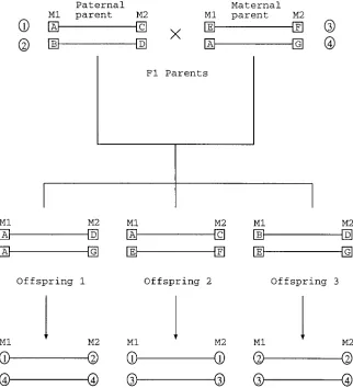
in male and female meioses are the same (even though illustrated in Figures 1 and 2.
Figure 1.—Genotypes of two marker positions in an F2full-sib family with three
offspring (an example). Haplotypes of all individuals are known. Arrows indicate how alleles are coded with respect to their grandparental “line” origins. The paternal (maternal) haplotype of offspring be-comes a sequence of lines 1 and 2 (3 and 4). For an illustration, suppose that there is a QTL (q) between the markers and that each haplotype of the parents contains a different QTL allele (also numbered from 1 to 4) in that locus. The four QTL geno-types are then combinations of parental chromosomes and they show the follow-ing correspondence here: 135(A–C, E– F), 145(A–C, A–G), 235(B–D, E–F), and 245(B–D, A–G). Denote the recom-bination fraction between the flanking markers by rLR, and that between the QTL
and the left (right) flanking marker by rq1 (rq 2). By applying Equation 6, the prob-ability of QTL genotype 13 occurring in offspring 1 is given by ((1 2rq1)rq 23
rq1rq 2)/(rLR(12rLR)), that of 14 by ((12 rq1)rq 23(12rq1)(12rq 2))/(rLR(12rLR)),
that of 23 by (rq1(12rq 2)3rq1rq 2)/(rLR(12 rLR)), and that of 24 by (rq1(12rq 2)3(12
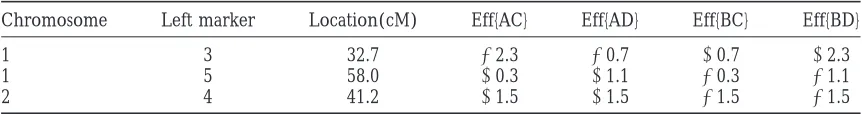
Van Ooijen (Centre for Biometry Wageningen, CPRO-DLO, The Netherlands). We considered two 100-cM long chromosomes, both having 11 evenly spaced mark-ers, at every 10 cM. The simulated trait had a genetic (QTL) variance 4.47 and a phenotypic variance 6.35, resulting in heritability 0.7. Two sets of parental crosses were generated: In the first set the parental mating type was fully informative (AB3CD) at all marker loci, and in the second set the degree of informativeness, as well as the corresponding linkage phases, varied from locus to locus. The simulated true underlying parental cross in the second set is shown in Figure 3; it is underlying in the sense that after the simulation this information was “forgotten” and not used in the Bayesian analyses (as explained below). The genotype-specific phenotype effects and the locations of the three simulated QTL can be found from Table 2. All haplotypic assignments in the offspring were assumed unknown. In the statisti-cal analyses, three specifications regarding the amount of parental information were considered: (1) All geno-Figure 2.—Genotypes at two marker positions in a
back-cross family with one offspring (an example). Haplotypes of types and haplotypic assignments in parents were as-all individuals are known. Arrows indicate how as-alleles are sumed known; (2) all genotypes were assumed known coded with respect to their grandparental origins. Paternal
but their phases unknown in parents; and (3) all paren-parent of backcross progenies is also one of the grandparen-parents,
tal and grandparental marker information was assumed
i.e., code 3 means {1 or 2}. In case fixed (grandparental) lines
unknown (missing). The performance of our method are assumed, codes 2 and 3 can be replaced by 1, and thus
paternal meioses are not considered in the QTL genotype was compared to that of “all-markers” interval mapping probability calculations at all, i.e., if an offspring chromosome (IM;MaliepaardandVan Ooijen1994) and to multi-inherited from the nonfounder parent, here the maternal
ple QTL mapping with two background controls parent, is of type 1–2, then for a QTL between the markers
[MQM/02; both implemented in the MAPQTL pro-the genotype probabilities of types 1X and 2X are given by
gram ofVan OoijenandMaliepaard1996; MAPQTL (12rq1)rq 2/rLRand rq1(12rq 2)/rLR, respectively; here X
indi-cates the other (not considered) allele. (tm) version 3.0; CPRO-DLO, Wageningen, The Neth-erlands]. Note that in the IM and MQM methods the genotypes and the linkage phases in parents must be SIMULATION ANALYSIS
known.
In addition, the simulated data in which each QTL To test the performance of this method, an
outcross-had four alleles were analyzed (in cases 1 and 3), having ing F2population consisting of Nind5200 offspring was
generated by a simulation program provided by J. W. incorrectly assumed fixed grandparental lines (where
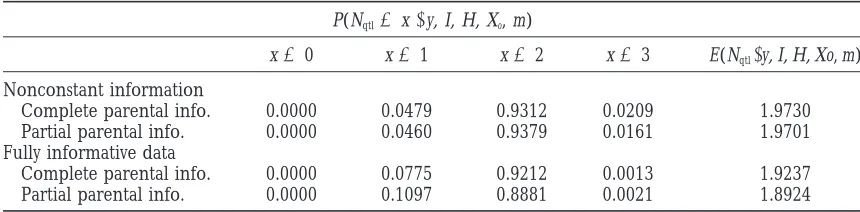
TABLE 2
The locations and the individual phenotypic effects (eff{·}) of different heterozygous genotypes of the three simulated QTL
Chromosome Left marker Location(cM) Eff{AC} Eff{AD} Eff{BC} Eff{BD}
1 3 32.7 22.3 20.7 10.7 12.3
1 5 58.0 10.3 11.1 20.3 21.1
2 4 41.2 11.5 11.5 21.5 21.5
The left column refers to the chromosome in which the considered QTL is located. The next column refers to the nearest left flanking marker of the QTL in the chromosome. Location is the distance (in centimorgans) between the QTL position and the leftmost marker in the linkage group. Parental mating type (maternal parent3paternal parent) in all three QTL positions is AB3CD.
TABLE 3
The rangesR(·) of the proposal distributions for different parameters, the corresponding proposal probabilities, the numbers of iterations, and the indices of the background control markers
from other chromosomes, which were used in the simulation analyses
R(lq) R(a) R(s) R(bqj) R(ckj) pa5pd No. of iterations BGCs
Chromosome 1 2.0 1.0 0.2 1.5 2.0 1/3 5,000,000 3
Chromosome 2 2.0 1.0 0.2 1.5 2.0 1/3 5,000,000 4
BGCs, background control markers.
grandfathers were assumed to originate from the same around 9 hr. The initial value for the number of QTL was three, and the corresponding locations were 20.0 line). This was done to see how this erroneous
assump-tion influences the results. cM, 50.0 cM, and 80.0 cM. The Poisson mean (hyperpa-rameter) was set to l 52 and the maximum number In all Bayesian analyses described here, our
C-pro-gram implementing a Metropolis-Hastings chain was of QTL (in the analyzed chromosome) to three. The residual standard deviation was chosen to be uniform run 5,000,000 cycles in a Pentium II/266MHz computer.
No values were deleted because of burn-in, but the chain over the range [0.0, 2.55], the right endpoint being equal to the phenotypic standard deviation estimate was thinned so that only every fifth iteration was saved,
resulting in 1,000,000 sampled values for each parame- from the data. The prior of the intercept was taken to be uniform on [213, 13], those of the QTL genotypic ter. After a preprocessing stage (seeappendix a),
back-ground controls were chosen. When analyzing a real regression coefficients were independent normal distri-butions with mean zero and variance 100, and the prior data set, they can be determined by a single marker
regression or by performing several analyses. Here, how- of the background control genotypic regression coeffi-cients was uniform on [213, 13]. Finally, the prior of the ever, we simply chose marker 3 in chromosome 1 and
marker 4 in chromosome 2 as background controls. QTL locations was uniform over [0, 100]. The control parameter values used in the final analyses are given in Very likely, a few reanalyses would have led to the same
conclusion. As no covariates (age, sex, etc.) were used, Table 3. The proposal distribution for the genotypic effects (coefficients) was chosen to be N(0, 0.5) in cases there was a common intercept (r 5a and Bi 5 1 for
all i). The running times, in circumstances where there where the addition of a new QTL to the model was proposed.
was practically no other load in the computer, varied
c
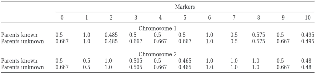
TABLE 4
The posterior distribution of the number of QTL and its expectation in four analyses of chromosome 1
P(Nqtl5x|y, I, H, Xo, m)
x50 x51 x52 x53 E(Nqtl|y, I, H, Xo, m)
Nonconstant information
Complete parental info. 0.0000 0.0479 0.9312 0.0209 1.9730 Partial parental info. 0.0000 0.0460 0.9379 0.0161 1.9701 Fully informative data
Complete parental info. 0.0000 0.0775 0.9212 0.0013 1.9237 Partial parental info. 0.0000 0.1097 0.8881 0.0021 1.8924
“Complete parental info.” refers to the analysis where all parental genotypes and linkage phases were known and “partial parental info.” refers to the case where only parental genotypes were available.
In the IM and MQM/02 analyses, walking speed was that are not unique. These problems are described and set to 0.5 cM, which is the smallest admissible value in considered more in thediscussion.
the MAPQTL software. We used the same background Table 5 gives a brief summary of our findings concern-controls in MQM/02 as in the Bayesian analyses. ing the localization of QTL as suggested by the QTL intensities in Figures 4 and 5. The table makes direct reference to (approximate) posterior probabilities that RESULTS a particular chromosomal regionIof high
QTL-inten-sity concentration contains a given number of QTL. The Bayesian posterior QTL intensities (seeappendix
Also the corresponding posterior expectations are
cal-b) in chromosome 1, when all parental information was
culated. The analyses support quite strongly the hypoth-present (case 1) or when parental linkage phases were
esis of two QTL in chromosome 1. absent (case 2), are shown in Figure 4 (top) when all
In the analyses where all markers were fully informa-markers are fully informative, and Figure 5 (top) when
tive (Figure 4, top), the two posterior QTL-intensity marker information varies from marker to marker. The
graphs (from cases 1 and 2) became nearly identical, curves consisting of the pointwise medians and the 2.5
regardless of whether parental linkage phase informa-and 97.5% quantiles of the posterior distribution of the
tion was available or not. Both posterior QTL-intensity phenotypic effects of the four genotypes, as functions
graphs were nicely concentrated around the left QTL of the putative QTL location, are shown in the same
at 32.7 cM. The graphs surrounding the right (weaker) figures when all parental information is present (left),
QTL at 58 cM were much wider, and there was also or when parental linkage phases are unknown (right).
some bias to the left. However, the true simulated QTL Approximate posterior distributions of the number of
is still inside the regions [41 cM, 60 cM] and [41 cM, QTL in chromosome 1, obtained from these four
differ-63 cM] of elevated posterior QTL intensities. In this ent analyses, are shown in Table 4. The analyses where
case (Figure 5, top left), the MQM analysis performed all parental information was absent (case 3) are not
well in both QTL localizations in chromosome 1, but summarized in figures or in tables. This is because in
the IM analysis managed to localize only the left QTL. theory case 3 is not fully identifiable, resulting in
proba-(Note that the posterior QTL-intensity graphs covering bilistic summary measures (the posterior QTL intensity
and the posterior distribution of the number of QTL) the regions [41 cM, 60 cM] and [41 cM, 63 cM] are
TABLE 5
Approximate (posterior) probability (12exp{2eIlˆ (s)ds}) that a given chromosomal area
Icontains at least one QTL, calculated for different areasIin four analyses
Chromosome 1 I Length (I) P(NI
qtl$1|data) E(NIqtl| data)
Nonconstant information
Complete parental info. [22 cM, 35 cM] 13 cM 0.63 0.9955 Complete parental info. [52 cM, 60 cM] 8 cM 0.59 0.8975 Partial parental info. [23 cM, 38 cM] 15 cM 0.65 1.0411 Partial parental info. [40–49] and [57–61] 13 cM 0.57 0.8502 Fully informative data
Complete parental info. [28 cM, 37 cM] 9 cM 0.63 0.9881 Complete parental info. [41 cM, 60 cM] 19 cM 0.59 0.8933 Partial parental info. [28 cM, 37 cM] 9 cM 0.63 0.9858 Partial parental info. [41 cM, 63 cM] 22 cM 0.58 0.8681
The (posterior) expected number of QTL inI, calculated as the integral of the QTL intensity overI, is also determined. “Complete parental info.” refers to the analysis where all parental genotypes and linkage phases were known and “partial parental info.” refers to the case where only parental genotypes were available.
multimodal. This is apparently the same phenomenon of the fact that there is a highly informative marker very close to the right QTL, whereas this is not the case with that is typical to the LOD-score curve at marker points:
often there is more evidence, because of marker geno- the left QTL (see Table 6). As could be expected, the localization was somewhat less accurate when the paren-typing, against placing a putative QTL exactly at a
marker locus than against placing it somewhere tal genotypes or their linkage phases were not available. Consider next the estimation of the phenotypic ef-nearby.) The graph leaves somewhat uncertain why, of
the two modes, the one that is farther away from the fects, indicated by asterisks in Figures 4 and 5. As could be expected, the estimation was most successful in the true simulated QTL at 58 cM ended up being higher
in the first case. case (displayed in Figure 4, left) where marker informa-tion was complete and where complete parental infor-It can be seen from Figure 5 that the nonconstant
marker information analysis (case 1) results in high mation was available. In the case of nonconstant marker information, but still assuming complete knowledge of posterior QTL intensities surrounding both simulated
QTL in chromosome 1. The IM and MQM analyses the parental genotypes and linkage phases, the estimates were somewhat less accurate, with some of the true localized quite well the “left” QTL at 32.7 cM, but
local-ization of the “right” QTL at 58 cM was poor with both values being just outside the 95% credible boundaries (Figure 5, left). When analyzing real data, the true label-methods. Somewhat surprisingly, in the Bayesian
method, the left, more influential, QTL was not local- ing [i.e., assigning of the QTL genotypes (13, 14, 23, 24) to the true grandparental alleles] of the phenotypic ized as accurately as the right QTL when linkage phases
were available in parents. This may be a consequence effects is almost always unknown (except for the QTL
TABLE 6
Estimated informativeness of different marker loci of the simulated data set, with two degrees of parental genotype information
Markers
0 1 2 3 4 5 6 7 8 9 10
Chromosome 1
Parents known 0.5 1.0 0.485 0.5 0.5 0.5 1.0 0.5 0.575 0.5 0.495
Parents unknown 0.667 1.0 0.485 0.667 0.667 0.667 1.0 0.5 0.575 0.667 0.495
Chromosome 2
Parents known 0.5 0.5 1.0 0.505 0.5 0.465 1.0 1.0 1.0 0.5 0.48
Parents unknown 0.667 0.5 1.0 0.505 0.667 0.465 1.0 1.0 1.0 0.667 0.48
TABLE 7
Point estimates and their support regions from different analyses
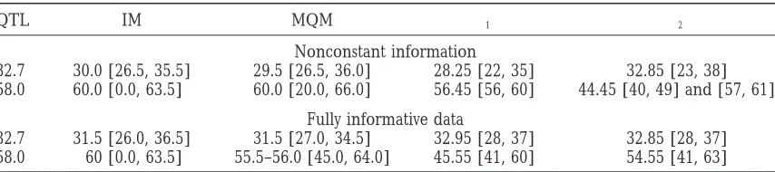
QTL IM MQM I1 I2
Nonconstant information
32.7 30.0 [26.5, 35.5] 29.5 [26.5, 36.0] 28.25 [22, 35] 32.85 [23, 38] 58.0 60.0 [0.0, 63.5] 60.0 [20.0, 66.0] 56.45 [56, 60] 44.45 [40, 49] and [57, 61]
Fully informative data
32.7 31.5 [26.0, 36.5] 31.5 [27.0, 34.5] 32.95 [28, 37] 32.85 [28, 37] 58.0 60 [0.0, 63.5] 55.5–56.0 [45.0, 64.0] 45.55 [41, 60] 54.55 [41, 63]
True QTL locations, their estimated locations and one-lod-support intervals from the IM and MQM analyses, and Bayesian point estimates (modes of the QTL intensity) together with suggested support intervals (I1) when
parental genotypes and haplotypes are available, and (I2) when no parental haplotypes are available (from
Table 5). LOD score was evaluated every 0.5 cM in the IM and MQM estimation. The posterior modes (intervals) were obtained with binlength 0.1 cM (1.0 cM), using all 5,000,000 sampled values inI1and 1,000,000 values
inI2. Note that in the IM and MQM analyses, there is no counterpart to estimates in columnI2.
genes that have been positionally cloned). If parental tion was absent, only the latter QTL resulted in a high (but broad) QTL-intensity concentration.
genotype and/or linkage phase information are miss-ing, the labeling of the genotypic effects according to the grandparental origin of the alleles also becomes
DISCUSSION nonunique in the simulated case. For this reason, when
comparing the phenotypic effect estimates with the true We have presented here a Bayesian procedure for mapping multiple QTL from incomplete outbred off-values used in the simulation, we have to make sure that
each estimate is matched correctly with a combination spring data, thus extending our earlier method ( Sillan-pa¨a¨andArjas1998) to a more general experimental of two grandparental QTL alleles. Such reassignment
of the QTL genotypes is indicated on the right-hand design. A test version of the software (written in C lan-guage) is available at http://www.rni.helsinki.fi/zmjs/. side of Figures 4 and 5 by circles. In chromosome 1,
note that the genotype labels are not consistent with The method is capable of handling situations where marker information from parents and/or grandparents each other in case 2.
The performance of the IM and MQM methods in the is missing in varying degrees, as well as cases where some of the marker information from the offspring is estimation of the phenotypic coefficients of the putative
QTL was not particularly good. Moreover, they do not unavailable. In contrast toSillanpa¨a¨andArjas(1998), the present model was not overparameterized, because provide confidence intervals for such point estimates.
Confidence intervals would have to be determined sepa- this did not seem to improve the mixing properties of the sampler.
rately, for example, by employing bootstrap techniques.
The point estimates of QTL locations and their sup- Following Sillanpa¨a¨ andArjas (1998), we use the posterior QTL intensity as a probabilistic summary mea-port regions are summarized in Table 7 for four
differ-ent analyses of chromosome 1. sure for the localization of QTL. During the MCMC sampling, we do not restrict the order of the QTL in any When considering chromosome 2 (which was
ana-lyzed only in cases 1 and 3), the posterior QTL-intensity way to label them. If order-based labeling is preferred, it can be established afterward from the MCMC realiza-graphs (see Figure 6) were all nicely concentrated
around the simulated true QTL at 41.2 cM, regardless tions. This is an alternative to imposing constraints on the MCMC simulation as was done, e.g., inSatagopan
of whether the markers were fully informative or not.
Also, the IM and MQM methods were able to localize et al. (1996),Satagopan and Yandell (1996),
Rich-ardsonandGreen(1997), and inUimariand
Hoes-the QTL at 41.2 cM quite well.
The performance of the analyses (cases 1 and 3), chele(1997).
We tested the performance of our method by using when it was incorrectly assumed that the grandparental
lines are fixed (pictures not shown), was quite poor in simulated F2data sets (two informativeness levels), with
varying degrees of parental marker information (three chromosome 1. The only exception was the case where
all parental information was available and all markers levels). It seems intuitively plausible, and it also became clear from our simulations, that the availability of paren-were fully informative. Then the simulated QTL at 32.7
cM was localized rather well, and there was also some tal linkage phase information is more important in the case where the markers are not fully informative. The indication of QTL activity around the QTL at 58 cM.
informa-Figure6.—The posterior QTL intensity in chromosome 2 when all parental haplotype informa-tion is known and the marker in-formation varies from marker to marker. The results from inter-val mapping (IM, solid line) and multiple QTL mapping with two background controls (MQM/02, broken line) are shown. The his-togram corresponds to the (ap-proximate) posterior QTL inten-sity over the chromosome, with binlength 1 cM. The left (right)
y-axis corresponds to the posterior
QTL intensity (LOD score). (*) The simulated true QTL.
Standardization of the phenotypic data is recom- uninformative areas, intensity graphs are much more spread out, or even biased in some direction.
mended before applying Bayesian QTL mapping in
practice. Then the same proposal windows and other The phenotypic effects can be estimated reliably only in chromosomal regions in which the posterior QTL control parameters can be applied to different data sets,
instead of performing separate test trials for each. An- intensity is sufficiently high. As an alternative to the locationwise posterior densities for phenotypic effects other advantage is that the numerical accuracy may be
improved because computers’ ability to store floating shown in Figures 4 and 5, the posterior density can be constructed as an expectation over several pointwise point numbers is maximal when dealing with numbers
between zero and one. values (of phenotypic effects), each being associated with a putative QTL location within a particular region The marker covariates can be chosen by an
applica-tion of simple linear regression at each marker (putative of high posterior QTL intensity. One such posterior density is shown in Figure 7.
QTL) position, omitting individuals whose genotype at
that locus was unknown (because data augmentation There appear to be two possible philosophies about how the indexing of QTL genotypes should be interpre-would need linkage phase information). In doing so,
one should pay attention to how much information a ted. Considering QTL genotype 13, for example, the first interpretation says that lines 1 and 3 are names potential covariate marker carries and how many
miss-ing values there are. If an interestmiss-ing region does not for the parental haplotypes. In this case the remaining uncertainty concerning linkage phase is in how the contain any fully informative markers, one can often
find two closely linked markers such that each marker grandparental alleles are assigned to these haplotypes. According to the second interpretation, lines 1 and 3 alone is informative only with respect to one (and a
different) parent. are names for the grandparental lines (alleles), and uncertainty is in the assignment of the parental haplo-Parental mating type is usually not constant in
out-crossing experiments. Thus a systematic application of types to these lines. Obviously, these two ways of thinking lead to different results only when there is some uncer-some index describing the proportion of informative
meioses locally present in the data will help the analyst tainty in the parental linkage phases. We have adopted here the first interpretation, even though the second to quantify the possibility of localizing a QTL in different
areas of the considered chromosome. One such mea- one is in some sense more fundamental in the context of QTL mapping.
sure is displayed in Table 6. The influence of marker
informativeness (cf. marker polymorphism in Krug- We stress that in situations where all parental informa-tion is missing (case 3) it will be problematic to assign
lyak 1997) can be seen clearly from our simulation
pheno-Figure7.—Approximate posterior distribution of the phenotypic effect of genotype 13 of the left QTL (chro-mosome 1), determined from the in-terval from 27 cM to 39 cM. All paren-tal information was available and all markers were fully informative.
type effects. In this situation, both parents have symmet- haplotype assignment can be made in a way that is with high probability consistent with that chosen at the refer-ric pairs of haplotype configurations that are a posteriori
equally likely to be the correct underlying mating struc- ence marker locus. If this informative marker is near a contemplated QTL, this technique will also facilitate ture. As a consequence, under these circumstances the
correspondence between QTL genotypes (13, 14, 23, the estimation of the corresponding phenotypic effects, by keeping the four haplotypic assignments (and thus and 24; cf. Figure 1) and their grandparental alleles is
not unique. In our program, the assignment can actually the corresponding QTL allele combinations) apart. A more negative aspect of this technique is that it works change from one iteration cycle to another within one
MCMC run, let alone in different runs. (In practice only locally, as simultaneous haplotype assignments at two or more marker positions might not agree with the such changes are rare because of the strong local
depen-dence between offspring and their parents and between true haplotype configuration. As a consequence, the estimation would need a new MCMC run for each such adjacent loci.) In case 3, the parental phase
reconstruc-tion can actually change suddenly in some region of local assignment.
the chromosome to a symmetrical mating type. (This M.S. thanks Matti Taskinen for his advice in the programming work, can only be checked from the simulated data.) Also the and Pa¨ivi Hurme and Outi Savolainen for many useful discussions about the designs. We are grateful to Johan Van Ooijen for providing resulting posterior QTL-intensity curves can differ in
his simulation program, which was used to generate test data sets, and such regions in different MCMC runs.
to Pekka Uimari and three anonymous referees for their constructive In cases 1 and 2, the very strong local dependency comments on the manuscript. This work was supported by a research structure between parents and offspring and between grant (no. 38352) from the Academy of Finland, and by the ComBi adjacent loci will in practice prevent such phase transi- Graduate School.
tions during the same MCMC run. Therefore, to avoid problems of this kind, we strongly recommend that at
least one of the parents should be genotyped in several LITERATURE CITED
marker loci along the chromosome, as equidistant as is Green, P. J., 1995 Reversible jump Markov Chain Monte Carlo com-possible. putation and Bayesian model determination. Biometrika 82: 711–
732. Locally, of course, if there is a fully informative
(refer-Haley, C. S., S. A. KnottandJ.-M. Elsen,1994 Mapping quantita-ence) marker, in case 3 we can also avoid such identifi- tive trait loci in crosses between outbred lines using least squares. ability problems and averaging in estimation by fixing Genetics 136: 1195–1207.
Heath, S. C.,1997 Markov chain Monte Carlo segregation and the assignments (segregation indicators) arbitrarily at
linkage analysis for oligogenic models. Am. J. Hum. Genet. 61: the reference marker and then using the fact that, as 748–760.
Hoeschele, I., P. Uimari, F. E. Grignola, Q. ZhangandK. M. Gage,
1997 Advances in statistical methods to map quantitative trait Thompson, E. A.,1994 Monte Carlo likelihood in genetic mapping. Stat. Sci. 9: 355–366.
loci in outbred populations. Genetics 147: 1445–1457.
Uimari, P.,andI. Hoeschele,1997 Mapping linked quantitative
Jansen, R. C.,1993 Interval mapping of multiple quantitative trait
trait loci using Bayesian analysis and Markov chain Monte Carlo loci. Genetics 135: 205–211.
algorithms. Genetics 146: 735–743.
Jansen, R. C.,1996 A general Monte Carlo method for mapping
Van Ooijen J. W.,and C. Maliepaard, 1996 Plant Genome IV. multiple quantitative trait loci. Genetics 142: 305–311.
Abstract at: http://probe.nalusda.gov:8000/otherdocs/pg/pg4/
Jansen, R. C.,andP. Stam, 1994 High resolution of quantitative
abstracts/p316.html/. traits into multiple loci via interval mapping. Genetics 136: 1447–
Wijsman, E. M.,1987 A deductive method of haplotype analysis in 1455.
pedigrees. Am. J. Hum. Genet. 41: 356–373.
Jansen, R. C., D. L. JohnsonandJ. A. M. Van Arendonk,1998 A
Zeng, Z-B.,1993 Theoretical basis for separation of multiple linked mixture model approach to the mapping of quantitative trait loci
gene effects in mapping quantitative trait loci. Proc. Natl. Acad. in complex populations with an application to multiple cattle
Sci. USA 90: 10972–10976. families. Genetics 148: 391–399.
Zeng, Z-B.,1994 Precision mapping of quantitative trait loci.
Genet-Janss, L. L., G. R. ThompsonandJ. A. M. Van Arendonk,1995
Ap-ics 136: 1457–1468. plication of Gibbs sampling for inference in a mixed major
gene-polygenic inheritance model in animal populations. Theor. Appl.
Communicating editor:Z-B. Zeng
Genet. 91: 1137–1147.
Jensen, C. S.,andA. Kong,1997 Blocking Gibbs sampling for link-age analysis in large pedigrees with many loops. Manuscript
avail-able at MCMC preprint service (http://www.stats.bris.ac.uk/ APPENDIX A: PREPROCESSING AND MCMC/).
PARAMETER ESTIMATION
Jensen, C. S.,andN. Sheehan,1998 Problems with determination of noncommunicating classes for Monte Carlo Markov Chain
Before the actual statistical analysis, the data go applications in pedigree analysis. Biometrics 54: 416–425.
through a preprocessing stage. In this process, we infer
Kao, C.-H.,andZ.-B. Zeng,1997 General formulas for obtaining the
MLEs and the asymptotic variance-covariance matrix in mapping as much of the marker genotype and linkage phase quantitative trait loci when using the EM algorithm. Biometrics
information as is possible by direct logical deduction 53:653–665.
from known parts of the family structure. The deduction
Knott, S. A., D. B. Neale, M. M. SewellandC. S. Haley,1997
Multiple marker mapping of quantitative trait loci in an outbred rules applied here (sequentially until there are no new pedigree of loblolly pine. Theor. Appl. Genet. 94: 810–820. assignments) are similar to the genotyping rules of
Wijs-Kong, A.,1991 Analysis of pedigree data using methods combining
man (1987). If grandparental genotypes are present, peeling and Gibbs sampling, pp. 379–385 in Computer Science and
Statistics Proceedings of the 23rd Symposium on the Interface, edited these deduction rules are first applied to the grandpar-byE. M. KeramidasandS. M. Kaufman. Interface Foundation, ents and parents, and then to the parents and offspring. Fairfax Station, VA.
In this process, sets of consistent parental mating types
Kruglyak, L.,1997 The use of a genetic map of biallelic markers
in linkage studies. Nat. Genet. 17: 21–24. are determined for each marker (see below) and they
Kruglyak, L., M. J. DalyandE. S. Lander,1995 Rapid multipoint are later repeatedly applied for the estimation. linkage analysis of recessive traits in nuclear families, including
Let us consider a multi-allelic marker in the chromo-homozygosity mapping. Am. J. Hum. Genet. 56: 519–527.
some to be analyzed, where, after the logical deductions,
Lander, E. S.,andP. Green,1987 Construction of multilocus
ge-netic linkage maps in humans. Proc. Natl. Acad. Sci. USA 84: the genotypes of the parents are still unknown. Further, 2363–2367.
consider the genotype or complete haplotype
imputa-Lin, S.,1995 A scheme for constructing an irreducible Markov Chain
tions for both parents by updating them one at a time. for pedigree data. Biometrics 51: 318–322.
Lin, S., E. ThompsonandE. Wijsman,1994 Finding noncommuni- In such situations, when the genotype of one parent cating sets for Markov Chain Monte Carlo estimation on
pedi-has been imputed, some offspring genotypes may in grees. Am. J. Hum. Genet. 54: 695–704.
fact uniquely determine the genotype of the other
par-Maliepaard, C.,andJ. W. Van Ooijen,1994 QTL mapping in a
full-sib family of an outcrossing species, pp. 140–146 in Biometrics ent. To avoid this and to make the sampler work more
in Plant Breeding: Applications of Molecular Markers, edited by
efficiently, genotypes of parents are considered jointly,
J. W. Van OoijenandJ. Jansen.CPRO-DLO, Wageningen, The
and they have to form a pair that is consistent with Netherlands.
Richardson, S.,andP. J. Green,1997 On Bayesian analysis of mix- the offspring genotypes. Therefore, we go through all tures with an unknown number of components. J. R. Stat. Soc.
possible allele combinations in parents, one at a time Ser. B 59: 731–792.
at each marker locus, and check whether any of them
Satagopan, J. M.,andB. S. Yandell,1996 Estimating the number of
quantitative trait loci via Bayesian model determination. Special is inconsistent with the offspring genotypes. All inconsis-Contributed Paper Session on Genetic Analysis of Quantitative
tent pairs are eliminated. In a backcross, one needs to Traits and Complex Diseases, Biometric Section, Joint Statistical
check an additional consistency in genotypes of related Meetings, Chicago, IL (available at ftp://ftp.stat.wisc.edu/pub/
yandell/revjump.html/). parents.
Satagopan, J. M., B. S. Yandell, M. A. NewtonandT. C. Osborn, Sometimes a block-update is preferred over a
single-1996 A Bayesian approach to detect quantitative trait loci using
site-update in MCMC applications to pedigrees (Kong
Markov Chain Monte Carlo. Genetics 144: 805–816.
Sheehan, N.,andA. Thomas,1993 On the irreducibility of a Markov 1991;Jansset al. 1995;Heath1997;JensenandKong
chain defined on a space of genotype configurations by a sam- 1997). This is because a local dependence resulting pling scheme. Biometrics 49: 163–175.
from inheritance constraints can be so strong that the
Sillanpa¨a¨, M. J.,andE. Arjas,1998 Bayesian mapping of multiple
quantitative trait loci from incomplete inbred line cross data. sampler in practice will be reducible during the available Genetics 148: 1373–1388. time if single-site updating dynamics are used (see
Shee-Sobel, E.,andK. Lange,1996 Descent graphs in pedigree analysis:
hanandThomas1993;Linet al. 1994;Lin1995;Jensen
application to haplotyping, location scores, and marker-sharing
reducible in some designs; seeJansset al. (1995). Single H*(t)
( j ) 5H( j )*new, and otherwise H( j )*(t)5H( j )*(t21). Here the
notation H*(t)
(j) refers to the family-block haplotype in
outbred family (F2 design) with many offspring is an
extreme example of this kind of strong dependence the jth marker in the tth round, while vector H*(t,new( j ))5
(H*(t)
(1), . . . , H*(t)(j21)H*new( j ) , H(j*(t121)1), . . . , H*(t(N)21)), vector
structure. Therefore, haplotypes for the entire family
are updated as one block (Step 2 below) at each marker. H*(t,j )5(H*(t)
(1), . . . , H*(t)(j) H(j*(t121)1), . . . , H*(t(N)21)), and
func-tion fj,i(H1*, H*2) 5 {p(GFj11,i(H*1)|GFj,i(H*2)) 3 p(GFj,i (In some cases, due to the dependency between
adja-(H*
2)|GFj21,i(H*1)) 3 p(GMj11,i(H*1)|GMj,i(H*2)) 3 p(GMj,i cent loci, good mixing properties of the sampler may be
(H*
2)|GMj21,i(H*1))}.
difficult to achieve, even when block-updating is applied
Step 3. Random walk proposals for regression parame-within one locus.)
ters are generated in three different blocks: (1) mean, In the following, we describe only those parts of the
environmental covariates, and residual standard devi-estimation algorithm that are different from those in
ation; (2) all QTL genotypic coefficients; and (3) all
Sillanpa¨a¨andArjas(1998; see also the graphical
rep-background control coefficients. Denote by L1 (L2)
resentation of the model therein):
the likelihood and by p1(p2) the normal density prior
Step 2. The following is repeated for each marker, j5 for the QTL genotypic coefficients evaluated at the 1, . . . , N: A new ordered genotype proposal (family- new (old) values. The proposals are accepted sepa-block) at the jth position is constructed as follows: rately for each block with probability min{1, L
13p1/
(L23p2)}. If accepted, thend(t)5 dnew, and otherwise
1. If one or both genotypes in parents are unknown, a
d(t)5 d(t21). (In block 3, the acceptance ratio is
evalu-consistent pair of genotypes is proposed. Each
consis-ated separately for each background control.) tent genotype-pair is considered as equally likely.
Step 4. Imputation for the missing background control 2. If unknown, their allelic origins are also proposed
markers is done as in Sillanpa¨a¨ and Arjas(1998) considering each configuration as equally likely.
except for the following: A consistent genotype pair 3. Incomplete offspring genotypes are completed by
is first proposed for the parents. Then all offspring taking one allele (with equal transmission
probabili-with a missing genotype in the corresponding back-ties) from each parent. These transmissions
simulta-ground control position are completed by sampling neously specify the allelic origins and the
grandpa-alleles according to Mendelian transmission probabil-rental origins, which are then updated accordingly.
ities. 4. Unknown allelic origins of known offspring
geno-types are determined by using deduction. Origins
of a homozygote can be assigned randomly, and APPENDIX B an offspring allele not found in one parent must
As in Sillanpa¨a¨ and Arjas (1998), we divide the originate from the other parent. If some origins are
chromosome into binsD1,D2, . . . ,DNbins, wherelˆjis the left uncertain, they are proposed with equal
prob-approximate posterior QTL intensity on intervalDj, ob-abilities.
tained from the Monte Carlo simulation of Ncycsiteration
5. Grandparental origins are determined for offspring
cycles. In a backcross or an F2intercross, let
alleles having a heterozygous parent, but are
ran-domly assigned for alleles inherited from homozy- l
Dx
j(d)5
o
Ncycs k51o
N(k)qtl
q511{l(k)q PDj, b(k)qx2m(k)q #d }
o
Ncycsk51
o
N(k)qtl q511{l(k)q PDj}
(7) gotes.
The family-block proposal H*new
( j ) is accepted, separately
for each marker j, with probability
be the empirical estimator of c.d.f. Dx
j(d) associated with min{1, p(x 5 x(t)|H*(t,new(j )), l(t), m, N(t)
qtl) the phenotypic effect of heterozygous QTL genotype x
at a putative QTL in binDjandm(k)q 5
o
Ngenx51 b(k)qx/Ngen. If 3pNindi51fj,i(H*(t, j21), H*(t,new( j )))/[p(x 5 x(t)|H*(t,j21), l(t), m, N(t)qtl)
fixation of QTL alleles in different grandparental lines
3pNind
i51fj,i(H*(t,j21), H*(t,j21))]}.
is assumed, we can use distribution functions similar to those presented for F2inSillanpa¨a¨andArjas(1998).