Dynamics of genetic variability in two-locus models of stabilizing selection.

Copyright 0 1994 by the Genetics Society of America

Dynamics of Genetic Variability in Two-Locus Models

of

Stabilizing Selection

Sergey Gavrilets*9t

and

Alan

Hastings*’19§

*Division of Environmental Studies, $Institute for Theoretical Dynamics, 5Center for Population Biology, University of California, Davis, California 95616 and tN. I. Vavilov Institute of General Genetics, 1 1 7 8 0 9 GSP-1, Moscow B-333, Russia

Manuscript received September 27, 1993 Accepted for publication June 23, 1994

ABSTRACT

We study a two locus model, with additive contributions to the phenotype, to explore the dynamics of different phenotypic characteristics under stabilizing selection and recombination. We demonstrate that the interaction of selection and recombination results in constraints on the mode of phenotypic evolution. Let Vg be the genic variance of the trait and C, be the contribution of linkage disequilibrium to the genotypic variance. We demonstrate that, independent of the initial conditions, the dynamics of the system on the plane ( Vg, C,) are typically characterized by a quick approach to a straight line with slow evolution along this line afterward. We analyze how the mode and the rate of phenotypic evolution depend on the strength of selection relative to recombination, on the form of fitness function, and the difference in allelic effect. We argue that if selection is not extremely weak relative to recombination, linkage disequilibrium generated by stabilizing selection influences the dynamics significantly. We demonstrate that under these conditions, which are plausible in nature and certainly the case in artificial stabilizing selection experi- ments, the model can have a polymorphic equilibrium with positive linkage disequilibrium that is stable simultaneously with monomorphic equilibria.

M

OST studies of the dynamics of quantitative char- acters have emphasized the ‘classical’ case ofweak selection on a character controlled by a large number of loci [reviewed in BARTON and TURELLI (1989)l. Yet, as reviewed in ORR and COYNE ( 1 992), the evidence that quantitative characters are controlled by many loci is not compelling-the possibility that many quantitative traits are controlled by only a few loci cannot be ruled out. In this case, selection on the individual loci underlying the trait may, in fact, be quite strong, so the role of recom- bination may be significant. Thus, studies of multilocus models where the fitnesses are chosen to reflect a quan- titative trait may be vital for understanding the behavior of natural systems.

However, the overwhelming majority of theoretical studies of the relationship between selection and recom- bination using multilocus population genetics models have focussed on equilibrium behavior [reviewed in

HASTINGS (1989) and NAG- (1992)l. Studies of dy- namics, both theoretical and experimental, may prove much more informative, especially if it cannot be a s sumed that systems are at equilibrium. Questions such as “How long does it take to approach an equilibrium?” and ‘What can be said about characteristics of the mul- tilocus system during the transient period?” have usually not been considered. The notable exceptions are the studies by LEWONTIN (1964), NAGW (1976,1977,1978, 1993) and HOPPENSTEAD (1976). These questions, how- ever, become very important if, for example, the time to reach the equilibrium is longer than the time interval during which the fitnesses can be considered as con- stants. For example, questions of dynamics become

Genetics 138: 519-532 (October, 1994)

paramount in any attempt to relate the predictions of the genetic models to laboratory experiments studying the dynamics of quantitative characters under selection [reviewed in HILL and CABALLERO (1992)l.

Modeling of dynamics has recently attracted attention in quantitative genetics ( e . g . , WAGNER 1984; BURGER 1986; KIRKPATRICK and LANDE 1989; LANDE 1991; BURGER

and LYNCH 1994). The emphasis of these studies has mainly been on the behavior of the mean values of quan- titative traits while the variances (and covariances) are assumed to be constant. To justify this simplification an assumption ofweak selection is invoked. However, when applying population genetics models to quantitative traits, particularly when considering experiments, the relevant circumstance is typically strong selection. Strong selection seems also to be typical in natural popu- lations (ENDLER 1986). Our previous analysis of some selection regimes (GAVRILETS 1993; GAVRILETS and

HASTINGS 1993, 1994a) has shown that qualitative and

quantitative characteristics of equilibria under strong se- lection are quite different from those under weak selection. We may expect that the same is true with re- spect to the dynamics.

Gavrilets and A. Hastings

absent. BULMER (1971, 1980) has developed a comple- mentary approach based on specific assumptions about the phenotypic and genotypic distributions [see TURELLI

(1988) and GAVRILETS and HASTINGS (1994b) for a mul- titrait generalization]. In the resulting model the change in the genotypic variance is attributed to the change in linkage disequilibrium, while, because of the assumption about a very large number of loci with small effects, the allele frequencies do not change. CHEVALET

(1988) generalized this approach for the case where the number of loci, alleles, as well as the population size can be finite. Nevertheless, this analysis still has two limita- tions. The first is that CHEVALET'S approach (as well as BULMER'S) describes the dynamics of unlinked loci and it is not clear how to generalize it for the case of linked loci. The second is that this approach is heavily based on the assumption of a multivariate normal distribution of the effects of the loci. This assumption, although typical in quantitative genetic models, still has to be justified (TURELLI 1984).

Thus, theoretical approaches which include linkage disequilibrium, as would be generated by strong selec- tion, and focus on dynamics rather than equilibrium behavior, are needed. In this study, we begin such a pro- gram of investigation, looking at the dynamics of stabi- lizing selection within the realm of two-locus models. Using a combination of approximate methods we shall obtain a quite complete picture of the dynamics, both in terms of allele frequencies and disequilibrium, as well as quantitative genetics parameters such as the mean or the variance. Our approach is also relevant to a recent em- phasis on bridging the gap between multilocus popu- lation genetics and quantitative genetics (TURELLI and BARTON 1990). The structure of this report is as follows. In the next section, we formulate a general model of

stabilizing selection on an additive trait controlled by

two diallelic loci. Then we consider the case of quadratic stabilizing selection and equal contributions of loci, where the analysis is the easiest and most complete. We then generalize these results by allowing other forms for the fitness function but still assuming equal con- tributions of the two loci. Finally we consider cases of quadratic stabilizing selection with unequal locus contributions.

GENERAL MODEL

We begin with a description of a general model of stabilizing selection on an additive quantitative trait de- termined by two diallelic loci. Assume that the alleles at locus i have effects a,/2 and

-ai/2,

and that ai # 0. We designate the larger of the ai as a1 and, without loss of generality, assume that a1 = 1, so that a p is the ratio of the effects of the alleles at the two loci. Let xl, x p , xg and x, be the frequencies of the gametes with the effects z1 = (1

+

a,)/2, z2 = (1 - a,)/2, z3 = (-1

+

a,)/2 and z, = ( - 1 - a p ) /2 on the trait. We shall use the standard

notation for these gametes: AB, Ab, aB, and ab. We as- sume that the fitness depends only on genotypic value so that the fitness, wv of an individual formed by ga- metes i and j and having phenotype zi = zi

+

zj can be represented as

where w is the fitness function. We assume that the fit- ness function w ( z ) has its optimum at zo, decreases monotonically from its optimum, and is symmetric about it, i . e . , w ( z - zo) = w ( zo - z) ; we scale w ( z) so that w ( zo) = 1. In this paper we shall assume that the optimum phenotype zo is zero, i. e . , it coincides with that of a double heterozygote. The effects of deviation of z,, from zero on the properties of equilibria have been analyzed in previous work (HASTINGS and HOM 1990; GAVRILETS and HASTINGS 1993). Let w, = wl1xI and W =

zi

wix, be the marginal fitness of gamete

i

and the mean fitness of the population. The dynamics of the gamete frequencies under selection and recombination are described by the standard relations

where r i s the recombination rate,

D

= xlx4 - %x3 is the standard linkage disequilibrium, and wI4 is the fitness of a heterozygote at both loci, w14 = w ( 0 ) . In

(2) the sign is minus for

i = 1 and

4

and is plus for i =

2

and 3.

Our analysis will present results in terms of quantita- tive genetics parameters, such as the mean value of the trait, i, the genic variance, Vg, and the contribution of the linkage disequilibrium, C,, to the genotypic variance of the trait under selection and recombination. Let

pi

be the frequency of the allele at the ith locus that increases the trait value (allele A at the first locus, and allele B at the second locus), qi = 1 -

p i .

Then

1

Dynamics of Genetic Variability 521

TABLE 1

Fitness values under quadratic stabilizing selection with equal contributions of the loci and zo = 0

BB Bb bb

AA 1 - 4s 1 "s 1

A a 1 - s 1 1 - s

aa 1 1 "s 1 - 4s

DYNAMICS UNDER QUADRATIC STABILIZING SELECTION WITH EQUAL CONTRIBUTIONS

OF THE LOCI

In this section we shall assume that the contributions of the loci are equal, L e . , that 'a = 1. Let the fitness function w ( z ) be a quadratic

W ( % ) = 1 - szz,

(4)

where s is the parameter measuring the strength of se- lection. Under quadratic stabilizing selection

(4)

the mean fitness of the population can be represented as

zl, = 1 - s( G

+

2'). The fitnesses of different genotypes in this model are given in Table 1. In this case the equi- librium structure is simple: the system evolves to one of the two monomorphic equilibria corresponding to the fixation of gamete A b or aB. What can be said about the dynamics of the phenotypic characteristics (3)?

The dynamics of the system can be elucidated because there are different timescales in the problem, even with- out making an assumption of weak selection. Details of our computations are in APPENDIX A. First we introduce new variables (KARLIN and FELDMAN 1970)

u = x, - x4,

v = $ - % , (5)

t = a j + x 4 - % - 3 E g .

In terms of these variables the phenotypic characteristics (3) are

i = 2u, ( 6 4

v , = l - u 2 - 3 , (6b)

c,

= t

-

u'

+

vz. (6c) Using these variables one can show that the change in the mean value of the trait in one generation is

Here we would like to emphasize two points. The first is that this equation is exact. The second is that surprisingly it is quite different from the equation A i =

-

( S s / G ) G f that one would derive from the standard formula in quantitative genetics A i = G(d In z i j / d i ) (LANDE 1979).

In our model the variable u, and hence the mean of the trait Z, monotonically evolves to zero (HASTINGS 1987). In APPENDIX A we show that u approaches zero

quickly and hence

i + 0 quickly. (8)

In other words, the evolution of the mean proceeds much faster than the evolution of other phenotypic characteristics ( c ) BULMER 1980), so that after a short time the absolute value of the mean is extremely small, and the other phenotypic characteristics have changed little.

We then concentrate on the dynamics of Vg and C,, under the assumption that i = 0. Note that if the op- timum value of the trait is about the population mean (a condition usually met in stabilizing selection experi- ments), then i

-

0 from the beginning. The changes in V and C, in one generation are AVg = -2vAv

-

(Av? = -2vAv, and AC, = At

+

2vAv

+

(Av)' = At

+

2vAv, where we have assumed that the change in v in one generation satisfies A v

<<

1. We can now use phase- plane methods to study these dynamics ( e . g . , CODDING TON and LEVINSON 1955). It is useful to approximate the dynamics in this phase plane by a differential equation to simplifjr the analysis. The qualitative features of the dynamics are not altered by this change to continuous time. Dividing AC, by AVg and substituting the differ- ential ratio dC,/dVg for the difference ratio AC,/AVg, we get the first order differential equation

dC, -

-?6,

-

1/S(v:

-

c:)

dVg -s(l - \)(Vg

+

C,) '

that approximates the dynamics of the components of the genotypic variance on the phase-plane ( Vg, C,). Note that the variables Vg and C, satisfy

"

(9)

0 5

v,"

1,

-5'

C L 5 (1 - (10)

The first inequality is obvious, while the second guar- antees the non-negativity of the gamete frequencies at

i = 0. In APPENDIX B, we describe the detailed phase-plane

analysis of (9), and we merely highlight some of the results here.

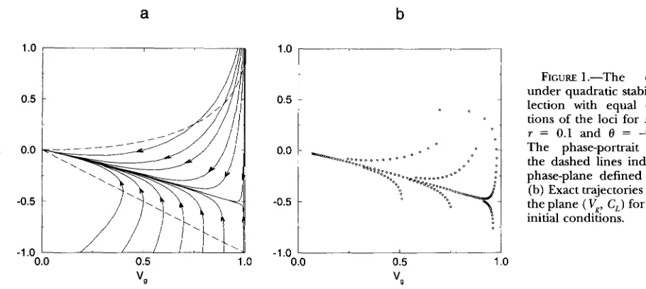
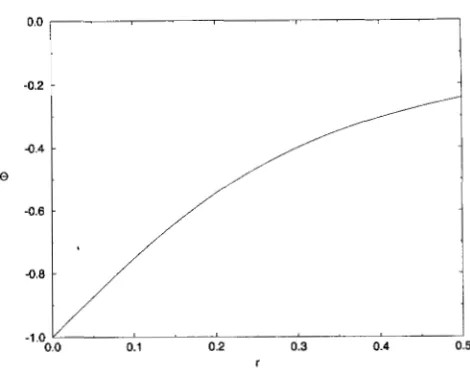
The most important and surprising feature of the dy- namics of (9) is that in the phase-plane the system quickly evolves to a line along which the dynamics are slower (see Figure 1 and APPENDIX B)

.

The line to which the system evolves is very close to the straight line given by the equation C, = OVg, where 0 < 0. It connects two equilibria of (9): the stable equilibrium (0,O) and the unstable equilibrium (1, 0). The former corresponds to the stable monomorphic equilibria of ( 2 ) with fixation of gamete Abor d. The latter corresponds to the unstable polymorphic equilibrium of ( 2 ) with allele frequencies of one half and a negative linkage disequilibrium of

D

= 0/4. At this equilibrium the contribution of linkage disequilib rium to the genotypic variance is

a

Gavrilets and A. Hastings

b

-1.0

‘

0.0 0.5 1 .o -1.0 0.0 L

v,

If selection is very weak (ie., if s

<<

r )

,

then 8 = 0, and the dynamics of the system correspond to that one studied by

NAGW (1976, 1977, 1978, 1993) and HOPPENSTEAD

(1976): there is a quick movement towards the so-called “quasi-linkage equilibrium” state with slow evolution of al- lele frequencies afterward. Our findings show that a similar separation of timescales takes place in general even with- out assuming weak selection (

Q

CHEVALET 1988). However, the population is not at linkage equilibrium (unless s

<<

r )

.

In our model, the population evolves to a monomorphic state, but during the evolution it is characterized by some level of negative linkage disequilibrium. While both the genic variance

%

and the contribution of linkage disequi- librium C, decrease, their ratio CJ

Vg

is about the same as at the unstable polymorphic equilibrium. Even moderately strong selection is sufficient to produce high levels of link- age disequilibrium at this state (GAVRILETS 1993). This equi- librium is unstable but nevertheless determines the mode and as we shall see below the rate of the evolution. If one ceases selection, than we expect to observe an increase in the genotypic variance to the level of the genic variance as recombination destroys negative linkage disequilibrium. The fact that the ratio CJV, does not change with time implies that the ratio of the genotypic variance after all disequilibrium was destroyed to the genotypic variance at the moment when selection stops, is independent of the time when selection was ceased (and equals 1

/

(1

+

8) )

.

The existence of different timescales in the model allows us to analyze the rate of evolution directly

(CJ:

CHEVALET 1988). As soon as a trajectory approaches the line C, = 8Vg, we can assume that C, = OV,. Ap- proximating the change in the genic variance in one generation AV, by the derivative dVg/dT, we get a single equation that describes how Vg changes with time

T:

dV - SV&l - V,)

-g =

d T 1 - SVE

.

(12)

where S = s(1

+

8) is a single parameter that deter-

FIGURE 1 .-The dynamics under quadratic stabilizing se- lection with equal contribu- tions of the loci for s = 0.15, T = 0.1 and 8 = -0.54. (a) The phase-portrait of (9); the dashed lines indicate the phase-plane defined by (10). (b) Exact trajectories of (2) on the plane ( Vg., C,) for different initial conditlons.

0.5 1 .o

v g

mines the rate of evolution. Note that the denomi- nator in the right-hand side of (12) is the mean fitness of the population evaluated at i = 0 and C, = 8Vg.

Equation (12) has a simple integral

where cis a constant that depends on the initial con- ditions. One can use (13) to find the time that it takes to reach some specified level of the genic variance starting from some other specified level. Figure 2A

illustrates the dependence of the rate of evolution on

S. Figure 2B shows how S depends on the strength of selection s and the recombination rate r. We see that, as expected, both strong selection and loose linkage increase the rate of evolution. These Figures show that

if the loci are moderately linked (say, with r 5 O.l), even strong selection can require more than a hun- dred generations to change the genic variance sig- nificantly. Using the fact that along the line C, = OV,,

C , = 8 V , , G ~ ( 1 + 8 ) V , , a n d W = 1 - s ( l + 8 ) V g , w e can also use Equations 12 and 13 for analyzing the dynamics of linkage disequilibrium, of the genotypic variance and of the mean fitness of the population.

OTHER MODELS OF STABILIZING SELECTION

Although our analysis is most complete in the case of equal locus contributions and quadratic selection, sub- stantial progress is possible in the analysis of other cases.

Equal contributions of the loci, arbitrary fitness func- tion: In this section we again assume the locus contri- butions are equal, but the form of fitness function is arbitrary. If a2 = 1, then the genotypic value can only be equal to 0 , T1, T2, and the fitness function can be completely characterized using only two parameters,

Dynamics of Genetic Variability 523

A

300.0

200.0

T

100.0

.

0.0

0.00

0.02

0.04

0.08

0.06

0.1

0

S

0 . 2 5 '

RGURE 2.-Influence of the parameters of the model on the rate of evolution. (A) The time that it takes to change the genic variance Vg from 0.95 to 0.05, from 0.9 to 0.1, and from 0.75 to 0.25 respectively. (B) The value of

S

as function of the intensity of selection s and the recombination rate r.

in a number of papers (e.g.,

BODMER

and FELSENSTEIN Result 1: If

2p

5 8, then the only possible stable equi- 1967; KARLIN and FELDMAN 1970). This special case libria are fixation equilibria xr = 1 or xs = 1.

I f 2 p

>

has not been analyzed in detail. The following result S and selection is sufficiently strong relative to linkage, summarizes the properties of stable equilibria of (2) then in addition to these fixation equilibria which

524

TABLE 2

Fitness values under arbitrary symmetric stabilizing selection with

equal contributions of the loci and zo = 0

B B Bb 66

A A 1 - 6 1 - P I

A a 1 - P 1 1 - P

a a 1 1 - P 1 - 6

TABLE 3

Fitness values in the symmetric fitness model

B B Bb bb

A A 1 - 6 1 - P

A a

1-CY

a a 1-CY 1 - Y 1 - P 1 1 - 6 1 - Y

equilibrium with allele frequencies equal to one half and positive linkage disequilibrium.

In APPENDIX A, we present the proof of this Result and

describe how the properties of the equilibria and the outcome of the evolution depend on the parameters. The stable polymorphic equilibrium whose existence was stated in Result 1 deserves to be discussed in some detail. Previously we have shown that if the contributions of the loci are different, than strong stabilizing selection can maintain variability in two ( GAWULETS and HASTINGS

1993) or many (GAVRILETS and HASTINGS 1994a) loci. Re-

sult 1 shows that the assumption about non-equal con- tributions of the loci is not necessary. The condition

2p

>

S means that on the plane (z, w ( z ) ) the point

(1, w ( 1 ) ) lies below the straight line that connects the points (0, 1) and (2, w ( 2 ) ) , i.e., w ( z ) isconvex.Thiscan be satisfied, for example, in the case of a double trun- cation or if w ( z ) is a Gaussian fitness function. The poly- morphic equilibrium exists simultaneously with two

monomorphic equilibria and, hence, the outcome of evolution depends on the history. Contrary to what in- tuition about selection on a quantitative trait would sug- gest, this equilibrium has a large level of positive linkage disequilibrium, i . e . , there is an excess of gametes in the coupling phase. The population evolves to this equilib- rium only if initially the population is characterized by a high level of positive linkage disequilibrium, i.e., the gamete pool consists mainly of gametes AB and ab with a small proportion of gametes A b and aB. Such “initial conditions” are plausible in selection experiments when the line subject to selection is produced from the initial cross of two highly inbred lines (with the genotypes

AB/AB

and ab/ab)

.

In other cases the population evolves to mono- morphic equilibria. A possibility of simultaneous stability of a polymorphic equilibrium and monomorphic equilibria in a different special case of the general symmetric model was demonstrated in (FELDW and LIBEW 1979).

If the contributions of the loci to the trait are equal, the mean value of the trait imonotonically evolves to the

1 .o

0.5

1

v,

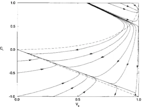
FIGURE 3.-The phase-portrait of (14) for r = 0.01,

p

= 0.35, 6 = 0.40. The dashed lines indicate the phase-plane defined by (10).

optimum (HASTINGS 1987). One can easily derive an ana-

log of Equation

7,

which again is different from the equa- tion that one would derive from the standard formula in quantitative genetics A f = G(

a

In w / d i ) . In APPENDIX A we show that i approaches zero quickly and that after some short time (typically about ten to fifteen generations) the change in the components of the genotypic variance on the phase plane ( Vg, C,) can be approximated by the first order differential equation

As

before the variables Vg and C, must satisfy the in- equality (10). The transient dynamics of the compo- nents Vg and C, of the genotypic variance have two quali- tatively different regimes. The first one corresponds to the evolution towards a polymorphic equilibrium, while the second one corresponds to the evolution towards one of the two possible monomorphic equilibria. We shall consider these regimes separately. On the phase- plane ( Vg, C,) with the variables satisfying (10) the poly- morphic equilibrium, which exists and is stable if 2p >

6 and selection is sufficiently strong relative to recom- bination, is given by the point (1, C 3 , where C: > 0 solves the numerator of Equation 14. The system evolves to- ward this state only if initially it belongs to the domain of attraction of this equilibrium. One can show (see AP-

PENDIX B and Figure 3) that the domain of attraction of

Dynamics of Genetic Variability 52.5

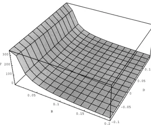
FIGURE 4 . T h e time that i t takes change the genic variance V, from 0.95 0.05 as function of .Band 9

to to

disequilibrium does not exist or that the initial condi- tions do not belong to its domain of attraction. In this case the dynamics of the system are similar to those in the case of quadratic stabilizing selection: the system quickly evolves to a line along which the dynamics are slower (see Figure 3 and APPENDIX B). This line is very close to the straight line C, = 8VK, where as before 8 is the contribution of linkage disequilibrium to the geno- typic variance at an unstable polymorphic equilibrium with allele frequencies one half and negative linkage disequilibrium. The value - 1 5 8 I 0 can be found as a solution of a cubic algebraic equation defined by the numerator of (14) with V, = 1.

As soon as a trajectory approaches the line C,, = OV,, we can assume that C,-

-

OV,. Approximating the change in the genic variance in one generation AVR by d V J d T , we get a single equation that describes how V, changes with time

T:

A = dV -3V,(l

-

V,)(l

+

Y V g )

d T 1

-

."V,

-

f l f l i / 2 (15)

where.3'= p ( l

+

O ) , L Z = (6/4p

-

1 ) ( 1

+

8). Note that the denominator in the right-hand side of (15) is the mean fitness of the population evaluated at 5 = 0 and

C, = OV,. Equation 15 has an integral

- 1

+

.w+

. m / 2

1 + 9 In(1 - V,)

+

In( V,)

Y +

3 / 2 1 + 9

-

_ln(1

₊

_m,)

₌

_-.m

₊

_c,

where c is a constant that depends on the initial con- ditions. If 6 = 4p (which is the case for quadratic sta- bilizingselection), then g= 0 , and Equations 15 and 16

reduce to Equations 12 and 13 correspondingly. One can use ( 1 6) to find the time that it takes to reach some specified level of the genic variance. Figure 4 illustrates the dependence of the rate of evolution on .Hand %.

One can see that the rate of evolution depends on %only weakly. As before, we can also use Equations 15 and 16 for analyzing the dynamics of C,,

G

and W .

Non-equal contributions of loci; quadratic

stabilizing

selection: In this section we shall assume that the con- tributions of the loci are different, i.e., that a2

<

1, and that the fitness function is quadratic (4). The equilibria in this model were analyzed in CAWLETS and HASTINGS (1993). Both equilibrium and transient behavior in this model are more complicated, but we still can get some analytical results. In APPENDIX A we show that on the phase-plane (u, v ) the trajectories of the system quickly approach the line u = -kv, where k is a positive value that depends on the parameters of the model. This im- plies that on the phase-plane (

PI,

p2)

the trajectories of the system quickly approach a straight line that passes through the point (Vi, %). On the phase-plane (5, V,) the trajectories of the system quickly approach the curve

where K, which is positive, depends on k and up. Along this curve

where V,,; = 2afp;q; is the contribution of the ith locus

S. Gavrilets and A. Hastings

1 .o 1 .o

0.5 -

PI 0.5 CL 0.0 -

-0.5 -

0.0

0.0 0.5 1

.o

-1.0 0.0 0.5 1

.o

.

1.0 I 1

0.0 I I

0.0 0.5 1 .o

B

CL

C

C L

-0.2

‘

I

0.0 0.5 1

.o

“g

0’25

7

I

J

-0.25

‘

I

0.00 0.50 1

.oo

D

0.5

CL 0.0

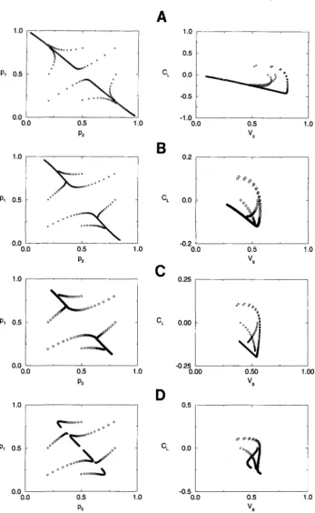
FIGURE 5.-Exact trajectories of ( 2 ) on the planes (

pl,

p,)

and ( Vg, C,) under quadratic stabilizing selection with s = 0.2 and unequal contributions of the loci. (A) r = 0.1, ap = 0.8, so that the system evolves to a monomorphic equilib- rium. (B) r = 0.1, ap = 0.4, so that the system evolves to a singly poly- morphic equilibrium. (C) r = 0.05, ap = 0.4, so that the system evolves to an “unsymmetic” doubly poly- morphic equilibrium. (D) r = 0.025, aq = 0.4, so that the system evolves to the “symmetric” doubly polymorphic equilibrium with

allele frequencies one half.

0.0

-

0.0 0.5 1

.o

-0.5 0.0 0.5 1 .o

P P v g

constant depends on

k

and a,. One can also derive an equation that describes the dynamics of

Vg,i

and C, on the phase-plane ( Vg,i, C , ) . This equation is a special case of the Appel equation. Instead of trying to analyze it we present results of numerical iterations of the full system

(2)

in the form of projections on the phenotypic space

(

p , ,

p,)

and ( Vg, C,)

.

The system has four possible re- gimes (GAVRILETS and HASTINGS 1993) that correspond to evolution toward: (a) one of two monomorphic equi-

libria, (b) one of two singly polymorphic equilibria, (c) one of two “unsymmetric” doubly polymorphic equilib- ria, and (d) a “symmetric” polymorphic equilibrium with allele frequencies one half.

As

expected, in each of these cases on the (

p , , p,)

plane we observe (see Figure

5 ) a quick movement towards a straight line with slow evolution afterwards. The dynamics on the (Vg, C,)

Dynamics of Genetic Variability 527

of these straight lines depend on the parameters of the model; increasing linkage decreases the rate of evolution.

EXAMPLE

In this section we consider how the theory developed in this paper can be used for analyzing results of artificial stabilizing selection experiments. The model we con- sidered was a two locus one, but it has been argued that a small number of loci can account for observable vari- ability in some quantitative traits (e.g., LANDE 1988; ORR

and COYNE 1992). Numerous papers with results of ar- tificial stabilizing selection experiments have been p u b lished (e.g., FALCONER 1957; PROUT 1962; GIBSON and THODAY 1963; SCHARLOO 1964; SCHARLOO et al. 1967; GIBSON and BRADLEY 1974; KAUFMAN et al. 1977; SOLIMAN 1982). In all these experiments the selection procedure used was double truncation: a small part

q

(usually be- tween % and %) of individuals with the phenotypes clos- est to the mean were selected. How is this translated into parameters of our model? Let the phenotype of an in- dividual, z , be the sum of the genotypic value, g, and a random normally distributed microenvironmental de- viation e having the zero mean and constant variance E .

In APPENDIX c we show that the mean fitness of a genotype

can be approximated as

This approximation is very good provided selection is at least moderately strong (say, with q

<

?4)

.

Several points concerning this approximation should be mentioned. The first is that the resulting fitness function is Gaussian. The second is that it does not depend on the proportion selected q (as long as

q

< ?A) and does not make any assumption about the number of loci. The third point concerns the strength of selection. Gaussian fitness func- tions are used in quantitative genetic models to describe natural stabilizing selection. The resulting mean fitness of genotypes in these models is w(g) = exp(-g2/2V), with V = V,

+

E, where V, is a parameter characterizing the strength of selection on phenotypes. It has been ar- gued that natural selection is typically weak with V, =

20E (TURELLI 1984) so that V = 21E. Expression (18)

shows that at least in the case of artificial stabilizing se- lection V

-

E . Note also that new data have indicated that natural selection can be as strong as artificial se- lec tion ( ENDLER 1986).

If initially the heritability coefficient h' =

?4,

C,

= 0 ,

and Vg

-

1 ( i. e . , the maximum possible level), then we can take E = 1. In the model with equal contributions of the loci this gives

p

= 1 - exp( -?A)

-

0.39, 6 = 1 - exp( - 2 )

-

0.86. Figure 6 shows how 8 depends on the recombination rate r for these values of

p

and 6. We see that even for unlinked loci the linkage disequilibrium generated by selection significantly decreases the phe-

O.O

I

-0.2

1

I

0.0 0.1 0.2 0.3 0.4 0.5

r

i

FIGURE 6.-The value 0 as function of the recombination rate r for

p

= 0.39 and S = 0.86.

notypic variance. Table

4

shows the time that it takes to reduce the genicvariance from 0.95 to 0.5 and from 0.99 to 0.5 for some specific r values computed using (16). We see that for unlinked loci the time to reduce the genic variance is very short. Finite population size and initial deviation of Vg from 1 will reduce it further. The difference between values in the two last columns of Table

4

can be interpreted as the time interval during which there are no visible changes in the phenotypic characteristics. One can see that a decrease in recom- bination rate increases this time. LEWONTIN (1964) dis- covered this effect in numerical simulations.

DISCUSSION

Two important points have traditionally been ne- glected in most theoretical studies of the evolution of multilocus systems. The first is the linkage disequilib- rium that is expected to be generated by selection. The second is the transient behavior of different character- istics of populations such as genetic variability. In this paper we have gained insight into these questions using the simple but nevertheless important two locus model of stabilizing selection. The results we have obtained confirm our previous conclusion (GAVRILETS 1993; GAWLETS and HASTINGS 1993, 1994a): linkage disequi-

S. Gavrilets and A. Hastings

TABLE 4

Influence of the recombination rate on the dynamics

r 0 TVc=0.95- VE=05 TVr=0.9% V,=O.5

0.50 -0.24 0.30 0.65 5 7

0.10 -0.75 0.10 0.21 23 35

0.01 -0.97 0.01 0.02 288 448

Our results demonstrate that if the loci are moder- ately linked, even strong stabilizing selection can require more than a hundred generations to change the genic variance significantly. This result has important impli- cations for selection experiments and for the mainte- nance of genetic variability. Stabilizing selection experi- ments typically do not last more than tens of generations and employ strong selection. So our results imply that if

dramatic reductions in variability occur, drift may in fact be more important than selection. When thinking about natural systems, it is unreasonable to expect that environ- mental conditions and populations remain constant over time scales of hundreds of generations. Our results imply that over shorter time scales, stabilizing selection will not have time to eliminate variability. Thus, the fact that at equilibrium variability cannot be maintained under stabi- lizing selection may be irrelevant-at time scales appropri- ate for some natural systems, variability is maintained.

A counter-intuitive conclusion of our analysis is that under conditions, which are plausible in artificial sta- bilizing selection experiments, the model can have a stable polymorphic equilibrium with positive linkage dis- equilibrium. This equilibrium is stable simultaneously with monomorphic equilibria. In this case the outcome of the evolution depends on the initial conditions. The approach we have developed allows us to use informa- tion about dynamics of observable characteristics of ge- netic systems under selection for testing hypotheses about properties of these systems. To have more prac- tical value this approach should be generalized for the case of more than two loci and of finite population. Our preliminary numerical analyses have shown that some of the conclusions of this paper are valid in these more complex situations.

The main effects described in this paper are related to earlier conclusions of LEWONTIN (1964), BULMER

(1971, 1974, 1980) and CHEVALET (1988). LEWONTIN (1964) numerically simulated stabilizing selection on an additive quantitative trait determined by 5 loci. He found that at first there is a rapid change both in allele frequencies (that brings the mean phenotype close to the optimum) and in linkage disequilibria. After this, allele frequencies and linkage disequilibria change slowly and this rate of change reduces with increases in linkage (reductions in recombination). We have shown how these changes are related to each other and to the parameters of the model by providing an analytical treat- ment of aspects of a two-locus model. BULMER (1971,

1974) considered a model in which selection does not change allele frequencies (due to an assumption about an effectively infinite number of loci with very small ef- fects). He found an equation that described the dynam- ics of the linkage disequilibrium component if the loci are unlinked, and proposed an approximation that al- lowed computation of the equilibrium value of this com- ponent in the case of linked loci. Our analyses of dy- namics have included both the case of linked loci and the case (obviously, more realistic) when allele frequen- cies change. Assuming multivariate normality of allele effects and no linkage, CHEVALET (1988) generalized Bulmer’s approach in many directions. In particular, he took into account the change in allele frequencies un- der selection, demonstrated the separation of times- cales, and analyzed the rate of evolution. Our analysis and conclusions are similar but are based on an exact multilocus genetic model and directly incorporate ef- fects of linkage.

The results described in this paper are also relevant to more abstract questions. Our finding about constancy of the ratio CJV, on the trajectories of the system seems to be related to the concept of “quasi-linkage equilibrium” introduced by KIMURA (1965). In Kimura’s numerical simulations a specific function of gamete frequencies (namely, Z = xIx4/x2xs) was nearly constant even when all gamete frequencies were changing. NAGYLAKI (1976) has shown analytically that this is true but only if

selection is very weak. Our results and a recent work by CHEVALET (1994) suggest that a function of gamete fre- quencies might be found that will behave as a “constant of motion” in more general situations. Also of some gen- eral interest may be the fact that in some sense the mode and the rate of the evolution in the model considered are determined by an unstable equilibrium.

We are grateful to CHUCKCOXWELL who made numerical simulations that inspired this work. We thank SALLY OTTO for helpful comments on the manuscript. This work was supported by U.S. Public Health Service Grant RO1 GM 32130 to A.H.

LITERATURE CITED

BARTON, N. H., and M. TURELLI, 1989 Evolutionary quantitative genetics-how little do we know. Annu. Rev. Genet. 23:

BODMER, W. F., and J. FELSENSTEIN, 1967 Linkage and selection: theo- retical analysis of the deterministic two locus random mating model. Genetics 57: 237-265.

BULMER, M., 1971 The effects of selection on genetic variability. A m .

Nat. 105: 210-211.

BULMER, M., 1974 Linkage disequilibrium and genetic variability. Genet. Res. 23: 281-289.

BULMER, M., 1980 The Mathematical Theory of Quantitative Genet-

ics. Clarendon Press, Oxford.

BURGER, R., 1986 Constraints for the evolution of functionally coupled characters: a nonlinear analysis of a phenotypic model. Evolution 40: 182-193.

BURGER, R., 1993 Predictions for the dynamics of a polygenic char- acter under directional selection. J. Theor. Biol. 162: 487-513. BURGER, R., and M. LYNCH, 1994 Evolution and extinction in a

changing environment: a quantitative-genetic analyses. Evolu- tion (in press).

Dynamics of Genetic Variability 529

CHEVALET, C., 1988 Control of genetic drift in selected popula- tions, pp. 379-394 in Proceedings of the Second International Con- ference on Quantitative Genetics, edited by B. S. WEIR, E. J. EISEN,

M. M. GODMAN, and G . NAMKONG. Sinaur Assoc., Sunderland, Mass.

CHEVALET, C., 1994 An approximate theory of selection assuming a finite number of quantitative trait loci. Genet. Sel. Evol. (in press)

CODDINGTON, E. A,, and N. LEVINSON, 1955 Theory of Ordinary Dif-

ferential Equations. McGraw-Hill, New York.

ENDLER, J. A., 1986 Natural Selection in the Wild. Princeton Uni- versity Press, Princeton, N.J.

FALCONER, D. S., 1957 Selection for phenotypic intermediates in Dro- sophila. J. Genet. 5 5 551-561.

FELLIMAN, M. W., and U. LIBERMAN, 1979 On the number of stable equilibria and the simultaneous stability of fmation and polymor- phism in two-locus models. Genetics 9 2 1355-1360.

GAVRILETS, S., 1993 Equilibria in an epistatic viability model under arbitrary strength of selection. J. Math. Biol. 31: 397-410.

GAVRILETS, S . , and A. HASTINGS, 1993 Maintenance of genetic vari- ability under strong stabilizing selection: a two locus model. Genetics 134: 377-386.

GAVRILEE., S., and A. ~ G S1994a , Maintenance of multilocus vari- ability under strong stabilizing selection. J. Math. Biol. 3 2 287-302.

GAVRILETS, S . , and A. HASTINGS, 1994b A quantitative genetic model for selection on developmental noise. Evolution (in press). GIBSON, J. B., and THODAY, 1963 Effects of disruptive selection. VIII.

Imposed quasi-random mating. Heredity 1 8 513-524.

GIBSON, J. B., and B. P. BRADLEY, 1974 Stabilizing selection in constant and fluctuating environments. Heredity 33: 293-302.

HASTINGS, A., 1987 Monotonic change of the mean phenotype in two-locus models. Genetics 117: 583-585.

HASTING., A., 1989 Deterministic multilocus population genetics: an overview. Lect. Math. Life Sci. 20: 27-54.

HASTINGS, A., and C. HOM, 1990 Multiple equilibriaand maintenance

44: 1153-1163.

of additive genetic variance in a model of pleiotropy. Evolution

HILL, W. G . , and A. CABALLERO, 1992 Artificial selection experiments. Annu. Rev. Ecol. Syst. 23: 287-310.

HOPPENSTUU), F. C., 1976 A slow selection analysis of two locus, two allele traits. Theor. Popul. Biol. 9: 68-81.

K A R L I N , S., and M. FELDMAN, 1970 Linkage and selection: two-locus symmetric viability model. Theor. Popul. Biol. 1: 39-71.

GUM, P. F., F. D. ENHELD and R E. COMSTOCK, 1977 Stabilizing se- lection for pupaweight in Tribolium urrtaneum Genetics 87: 327-341.

KIMURA, M., 1965 Attainment of quasi linkage equilibrium when gene frequencies are changing by natural selection. Genetics 5 2

KIRKPATRICK, M., and R. U D E , 1989 The evolution of maternal char- acters. Evolution 4 3 485-503.

U D E , R., 1979 Quantitative genetic analysis of multivariate evolu- tion, applied to brain:body size allometry. Evolution 3 3 402-416.

U D E , R., 1988 Quantitative genetics and evolutionary theory, pp. 83-94 in Proceedings of the Second International Conference on Quantitative Genetics, edited by B. S. WEIR, E. J. EISEN, M. M. GODMAN, and G. NAMKONC. Sinauer Assoc., Sunderland, Mass. LANDE, R., 1991 Isolation by distance in a quantitative trait. Genetics

128: 443-452.

LEWONTIN, R. C., 1964 The interaction of selection and linkage. 11. Optimal model. Genetics 5 0 757-782.

Genetics 83: 583-600.

Genetics 85: 347-354.

Springer, Berlin.

Springer-Verlag, New York.

selection. Genetics 134: 627-647.

assessment. A m . Nat. 140: 725-742. 875-890.

NAG-, T., 1976 The evolution of one- and twdocus systems.

NAG-, T., 1977 The evolution of one- and tw~locus systems. 11.

NAGW, T., 1978 Selection i n One- and Two-Locus Systems.

NAG-, T., 1992 Introduction to Theoretical Population Biology.

NAG-, T., 1993 The evolution of multilocus systems under weak

Om, H. A., and J. A. COWE, 1992 The genetics of adaptation-a re-

PROUT, T., 1962 The effect of stabilizing selection on the time

SCHARLOO, W., 1964 The effect of disruptive and stabilizing selection on the expression of a cubitus interruptus mutant in drosophila. Genetics 5 0 553-562.

SCHARLOO, W., M. S. HOOGMOE~ and A. TER KUIW, 1967 Stabilizing and disruptive selection on a mutant character in drosophila. I. The phe- notypic variance and its components. Genetics 56: 709-726. SOUMAN, M. H., 1982 Directional and stabilizing selection for devel-

opmental time and correlated response in reproductive fitness in

Tribolium castaneum. Theor. Appl. Genet. 63: 111-116.

TURELLI, M., 1984 Heritable genetic variation via mutation-selection balance: Lerch’s zeta meets the abdominal bristle. Theor. Popul. Biol. 2 5 138-193.

TURELLI, M., 1988 Phenotypic evolution, constant covariances, and the maintenance of additive variance. Evolution 42: 1342-1347.

TURELLI, M., and N. BARTON, 1990 Dynamics of polygenic characters under selection. Theor. Popul. Biol. 3 8 1-57.

USPENSKY, J. V., 1948 Theory of Equations. McGraw-Hill, New York. WAGNER, G. P., 1984 Coevolution of functionally constrained characters:

WOLFRAM, S., 1988 Mathematica: A System for Doing Mathematics by

prerequisites for adaptive versatility. BioSystems 17: 51-55.

Computer. Addison-Wesley, Reading, Mass.

Communicating editor: W. J. EWENS

APPENDIX A

Exact dynamic equations: If a double heterozygote has the optimum phenotype, i . e . , z,, = 0, and the fitness function is symmetric, Le., w ( z - z,,) = w ( z , - z ) , the twdocus model of stabilizing selection on an additive trait reduces to the symmetric viability model analyzed in a number of papers (see BODMER and FELSENSTEIN 1967; KARLIN and FELDMAN 1970). Table 3 gives the fitnesses of different genotypes in this model. Here

6 = 1 - w ( 1

+

a2). We shall use the linear transforma- tion ( 5 ) . Note that - 1 5 u, v, t 5 1 and that the new variables satisfy

ff = 1 - w ( l - CY2),

p

= 1 - w ( l ) , y = 1 - w ( a , ) ,

We shall use these inequalities repeatedly. Using vari- ables u, v, t, the dynamics of the system are (KARLIN and FELDMAN 1970) :

1

u’ = : [A,,(t)u

+

AI2(t)v],

W

+

- ff ((1 - t ) 2

+

4 3 ) - r ( t

+

3

-

u2)

,

8

1

where

6

8 8

w

= 1 - - ((1

+

t ) 2

+

4u2) -

-

ff ((1 - t ) 2

+

4 3 )

(A24 - -

P

(1 - t2

+

4uv)

-

- Y (1 - t 2 - 42474,

and

S. Gavrilets and A. Hastings

equilibrium values of t (with u = v = 0 ) 6

A,,(t) = 1 - - ( 1

+

t) -

(P

+

Y)(l -

4

1 - t 2

2

4 f ( t )

=

~p

( t -

(A24 4P

(Y - P>(1

+

4

A d t ) = shows that if 6

<

2P, then there exists T, > 0 such that

for 0

<

T

<

r, this cubic has two solutions, say t , and

4

,

a

(P

+

Y)(l

+

0

t2 ( t , < t2) between t* and 1, and has no solutions if 6

>

2P.

Note that if T = 0, than

t,

= t*. The consideration of (A2f) the equation for t' - t shows that

t,

is unstable, while

6

is

4 2 ( t ) = 1 - - (1 - t) -

(Y - P)(1 -

4

stable. The critical value r, can be found as follows. At T = A21(t) = ₄

r, the algebraic equationsf( t ) = 0 and g( t )

=

df( t ) / d t =

2 4

One can use equations

( A 2 )

together with (6) to get dynamic equations in terms of the phenotypic charac- teristics f , Vg and C,.

Equal contributions of the loci: If the contributions of the loci are equal, then a = 0 , /3 = 7, and the dynamics of the system simplify to

((1

+

t ) 2

+

4u2) -

where

and

P

2

A,(t) = 1 - - (1

+

t). _(A30

HASTINGS (1987) showed that 0

<

A,( t ) < rlr. That means that u monotonically approaches zero and, hence, at equilibrium u = 0. The consideration of the difference A,, -

w

with u = 0 shows that

One can see that if 6 2 2P, then A , 2 W for all -1 5

t 5 1. Together with the fact that A , > 0 that means that

if 6 2 2/3, then I v' I > I u I , and, hence, v + T1. At an equilibrium with I v I = 1, t = - 1. Obviously, these equilibria correspond to fixation of gamete A b or aB. If

6 <

2P,

then there exists t* = 6/(4P - 6) > 0 such that I d > I v I , i f t < t * , a n d I v r I < IvI,ift>t*.Theformer case corresponds to the convergence of the population to one of two monomorphic equilibria. The latter case corresponds to a polymorphic equilibrium with v = 0 that exists and is stable provided t stays in the area where t

>

t*. The consideration of the cubic equation for

0 have a common root. This is possible if the resultant

R( f , g) of the polynomialsf and gis zero (USPENSKY 1948).

Hence, to find r, we need to solve the algebraic equation

R( f ,

g )

= 0, which is cubic in our case. Result 1 in the main body of this report summarizes our findings.

We have already proved that u approaches zero while I u I tends to one or zero depending on the parameter values and the initial conditions. Now we are going to show that u reaches its equilibrium value much quicker than u. Equations A3a and A3b can be represented as

is to unity, the slower the corresponding variables evolves. If both A,( t )

,

A,,( t )

<

W, i. e . , if the system evolves to a polymorphic equilibrium with u = u = 0 , t = t2, then Equations A3e and A3f show that A,( t ) < A,( t ) . Hence,

A,

<

A,,,

u / u + 0, and u reaches zero much quicker then

u. If A,,( t ) >

W,

i . e . , if the system evolves to a monomor- phic equilibrium with u = 0 , I v I = 1, t = - 1, then using

the first of the inequalities in (Al) one can show that

u' = A,u, ur = A,v where Ai = A,/w > 0. The closer

A i

~3 - A,(t) 2 - 1 - t (6

+ t(6

- 2P)) (A6a)

4

and

l + t

4

A,(t) -

W

5

-

(6

+

t(6 - 2P)). (A6b)

As the system evolves, I v I increases, and not later than when I v I = %, the t value becomes negative (see Al). Inequalities (A6) show that for negative t , A, lies farther from unity than A,,, and, hence again u reaches its equi- librium value much quicker then v. Note that (A6) to- gether with ( A l ) can be used to show that I u r - u I >

I v r - v I for all t values. Thus, we have shown that u

reaches its equilibrium value much faster than u. Non-equal contributions of the loci: In this subsec- tion we consider the model of quadratic stabilizing se- lection with unequal contributions of the loci. We are going to show that in this case the dynamics on the

( u , v ) phase-plane are characterized by quick move- ment to a straight line along which the dynamics are slower. The dynamics on the ( u , u) phase-plane are described by

Dynamics of Genetic Variability 531

A, = 1

-

-

S (3

+

3 4

+

4 q t - <@, (A*b) 4

with

h,

>

A , , while the corresponding eigenvectors are

(1

-

a;)(l

+

t)

vec, =

(1

-

a;)(l

+

t) vec, =

-4%-t-a;t-<Q

I}*

(A9b)

where

Q =

1

+

14a;

+

a:

+

8%t

+

8a:t

+

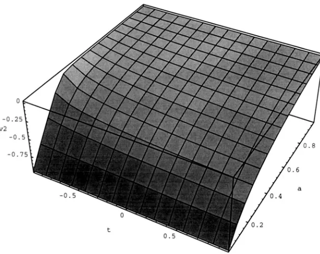
4ai&‘. Figure

7

shows that the eigenvector vec, that corresponds to the biggest eigenvalue practically does not depend on t, and hence is practically constant during the evolution. Let us introduce the

new

variables (x,

y):

(;)

= U(y”)’

where matrix

U

is constructed from the column vectors ( 0 , l ) and vec,. The dynamics of (x,

y)

are described by

(y”)’

= b - l A ( t ) U C ) . W

Matrix U’A(t)Uis a lower triangular matrix with diagonal elements A, and

h,

and a positive nondiagonal element. Since

4

>

A,

>

0 for all t, the first component ofvector (x,

y)

quickly approaches zero. In terms of the original variables

u and u this corresponds to quick movement of the system to the straight line represented by the second eigenvector.

FIGURE 7 . T h e first component ofvector vec2 as function o f t and a2.

APPENDIX

B

Approximate dynamics of (9): Equation 9 can be re- written as dC,/dV, = P( C,, V , ) / Q ( C,,

v,)

with the ob- vious interpretation. Simple methods for analyzing the phase portraits of such equations are well known

(e.g., CODDINGTON and LEVINSON 1955). The phase-plane of (9) is restricted by (10). The nullclines of VK are (i) V, = 1 and (ii) C, =

-

V,; the only nullcline of C, that belongs to the feasible art of the phase-plane is (iii) C, = r / s

-

+

r/s)‘

+ V i

(the nullcline C,. = r / s

+

v ( r / #

+

V;5 is not a part of the feasible area because on this nullcline C,

>

V,). Equation 9 has two equilibria at intersections of the nullclines:

(0,O)

and (1,

e),

where 8 is given by (1 1). The equilibrium point

(0,O)

is a stable node; the corresponding eigenvalues are equal to -s

and -r. This equilibrium of (9) corresponds to two

(9) are characterized by two different time scales with a quick movement towards the unstable manifold (rep- resented locally by the eigenvector ( - 1 - r / s , 1)) and a slow movement along this manifold. We are going to show that the same description of the dynamics is valid not only at a neighborhood of (1, 8) but on the whole phase-space, i.e., globally. Let us consider the value of d C , / d V , on the straight line that connects the equi- libria ( 0 , 0 ) and (1, 8). Using the fact that 8 satisfies the equation 78

+

s( 1 - 02)/2 = 0, one can show that dC,/dV,I c, = = ( 8 - 1 ) / 2 and, hence,

U V _{K I cl=ev,}

This means that the trajectories of (9) intersect the line C, = OV, from below. We can already see that all the trajectories of (9) enter a narrow area restricted by this line and the nullcline (iii) of C,. We can narrow this area further. Let us consider the value of d C I / d V , on the straight line C,, = 8Vg

+

E that is parallel with C, = OV, and lies a little higher then the latter. We are going to show that if E is greater then some small number, then

This means that the trajectories of (9) intersect the line C, = OV,

+

E from above. One can show that the

latter inequality is equivalent to

- E 2 8 - (1

+

8')E - 8(l

+

8)'V,(1 - V , )

<

0. (B2b)

In particular (B2b) is always satisfied for E 2 0.035. Inequalities (Bl-B2a) mean that trajectories of (9) enter a narrow area between lines C, = 8Vg and C, = OVg

+

E ( V,,

e),

where E ( V,, 8) < 0.035. Numerical iterations

show that all the trajectories of (9) approach the line

C, = 8Vg very closely (see Figure 1).

Approximate dynamics of (14): Let us assume that the polymorphic equilibrium (1, C 2 exists. One can easily see that the trajectories of (14) intersect the line C, = 4p/ (3p - (6 -

p ) )

- Vg from above. This line is

one of the three nullclines of V,; on it the term in the squared brackets in (14) is zero. Thus, if initially C, 5

4/3/ (3p - (6 -

p)

) - V,, then the system cannot evolve

towards this state. This shows that the domain of attrac- tion of the polymorphic state is small (see Figure 3).

Now let us assume that the system evolves toward one of the two monomorphic equilibria (with gamete A b or

U B

fixed). In phenotypic terms these equilibria are equivalent and are represented by the point ( 0 , O ) on the phase-plane ( V,, C,). This point describes the stable equilibrium of (14). Besides, (14) has an (unstable) equilibrium (1,

e),

where 8 < 0 , at the intersection of the nullcline V, = 1 of Vg with the nullcline of C, that is defined by the numerator of the right-hand part of (14). The equilibrium (1, 8) is approached only if VK = 1 ini- tially. The third nullcline of V, is given by V'

+ CIA

= 0. Let us consider the direction of the trajectories of (14)

on the line that connects ( 0 , O ) with (1, 8). If 6

>

2/3,

then inequality ( B l ) is still valid. If 6 5

2p,

then the derivative

dC,/dV, can change sign on the straight line C, = 8VK. However, one can still show that the trajectories of (14) enter a narrow area R restricted by two straight lines par- allel with C' = 8% one of which lies higher and another lower then C, = 8%. Let us consider the difference

Putting the terms in this difference over a common de- nominator (which is positive), one can see that the nu- merator can be represented as Num = f l (8, x, E )

+

df,( 8, x, E ) , where d = (S/4p) - 1 2 -% and fi are poly- nomials in 8, x and E . The consideration of the graph of

f2( 8, x, E ) using Muthemuticu software (WOLFRAM 1988)

shows thatf,

<

0 at E = -0.03 for all feasible 8 and x. That means that Num reaches its maximum at d = -X. The consideration of the graph of Num at d = -% and E =

-0.03 shows that it is negative for all feasible 8 and x. Al-

together this means that the trajectories of (14) intersect the line C , =

05

- 0.03 from below. In a similar way the consideration of the graph of f,(8,

x,

E ) shows that f2

>

0

at E = 0.10. That means that Num reaches its minimum at d = -%. The consideration of the graph of Num at d = -% and E = 0.10 shows that it is positive for all feasible 8

and x. Altogether this means that the trajectories of (14) intersect the line C, = 8%

+

0.10 from above. Thus, we have shown that all the trajectories of (14) enter a narrow area restricted by two straight C , = 8% - 0.03 and CI, = 8%

+

0.10. Numerical iterations show that all the trajec- tories of (14) approach the line C,. = 8% very closely.

APPENDIX C

The mean fitness of genotype under double trunca- tion: Let the phenotype of an individual,

z,

be the sum of the genotypic value, g, and a random normally dis- tributed microenvironmental deviation e having mean zero and constant variance E . Let the mean value of the trait be zero, and select for the next generation the in- dividuals with -zq < z < zq, where zq is the truncation point that corresponds to the proportion

q

selected. In this case the mean fitness of an individual with geno

value gis

u ( g )

= ~ ( z , -

g)/@

-

~ ( ( - 2 ~ - g)/

YC

~3, where @ ( x ) is the distribution function of a standard normal variable. In a vicinity of 0 (say for ?4 < @(x) < X),

@ ( x ) is excellently approximated by a linear function. This, together with the assumption that the phenotypic distribution is normal, allows us to approximate zq as

q m P , where P is the phenotypic variance. Now

zq/<E = qdrr/2(1 - h ) z , where h' = G / P is the heritability. Assuming that zJ<E < 1 (which is true, for example, for q < M and h' < %) and expanding

@ ( ( z q - g)/<@ and @( ( -zq - g)/<@ in Taylor series

at the point - g/<E, we finally find that the mean