Approximate thresholds of interval mapping tests for QTL detection.

Copyright 0 1994 by the Genetics Society of America

Approximate Thresholds of Interval Mapping Tests for QTL Detection

Ahmed Rebdi, Bruno Goffinet

and

Brigitte Mangin

INRA, Centre de Toulouse, Station de Biometrie et d’Intelligence Artificielle, Auzeville B.P. 27,

31326 Castanet-Tolosan, France

Manuscript received December 29, 1993 Accepted for publication June 1, 1994

ABSTRACT

A general method is proposed for calculating approximate thresholds of interval mapping tests for quantitative trait loci (QTL) detection. Simulation results show that this method, when applied to back- cross and F, populations, gives good approximations and is useful for any situation. Programs which calculate these thresholds for backcross, recombinant inbreds and F, for any given level and any chro- mosome with any given distribution of codominant markers were written in Fortran 77 and are available under request. The approach presented here could be used to obtain, after suitable calculations, thresh- olds for most segregating populations used in QTL mapping experiments.

T

HE use of genetic markers has opened new horizons for the identification and the location of Mende- lian factors involved in the expression of quantitative traits, so-called QTL (quantitative trait loci), in different segregating populations (backcross, F,,

. .

.). Recently, many efficient methods considering pairs of neighbor- ing linked markers have been developed (CARBONELL

et al. 1992; HALEY and KNOTT 1992; JANSEN 1992; K N M P et al. 1990; LANDER and BOTSTEIN 1989; MARTINEZ and CURNOW 1992; MORENO-GONZALEZ 1992) to infer the po- sition and the effect of a putative QTL lying between such markers. The interval mapping method described by LANDER and BOTSTEIN (1989) (LB) uses maximum likelihood estimation and provides a likelihood ratio test for the presence of a QTL between the markers con- sidered. The linearized method of KNMP et al. (1990)

and other related approaches (HALEY and KNOTT 1992) have been shown to be asymptotically equivalent to in- terval mapping ( R E B A ~ et al. 1994) (RGM)

.

The interval mapping test performed along the ge- nome could be defined as the supremum of a stochastic process and the distribution of the test statistic is not known in general. This has prevented many works for determining the exact threshold corresponding to a given significance level. LB have stated that, for a back- cross (BC) population of large size and in the case where the density of markers in the genome is infinite, the test varies according to the square of an Orenstein- Uhlenbeck process (LEADBETTER et al. 1983). They also gave a formula which is appropriate for threshold cal- culations under the conditions above and proposed to use extensive numerical simulations to determine the thresholds for intermediate marker densities. Thresh- old calculations for interval mapping tests in other prog- eny types, where more than one parameter are involved, have essentially been done using simulations (VAN OOIJEN 1992). RGM applied the DAVIES (1977) approach

Genetics 138 235-240 (September, 1994)

to get quite good approximations to the threshold of the interval mapping test in a BC population for a single interval of codominant markers.

In this report we generalize the approach previously described (RGM) for many intervals and other prog- enies for which there are two or more tested parameters. Simulations were also carried out to check the validity of the approximations used. We will first consider the case where the QTL is characterized by only one estimable parameter (its principle effect) which applies to BC and equivalent populations and then discuss the case where the QTL has additivity and dominance parameters, with application to F, (two parameters) and diallelderived populations.

THRESHOLDS IN THE SINGLE PARAMETRE CASE

The Davies approximation: Consider a chromosome of length P in recombination units having m

+

1

mapped markers from a BC population (equivalent to double haploid lines or F, testcross) and so m intervals of length

pi,(

i = 1

.

. .

m ) each. In this case the test for QTL detection involves only one parameter which is the principal effect of the putative QTL. The model used to estimate a (half the difference between genotypic values of QTL genotypes) is the same as that in RGM but any other parametrisation is equivalent. The thresholds cal- culated in this and following sections are thus suitable for flanking marker methods based on regression or likelihood analysis if only codominant markers are used. At each position x of the chromosome one can compute the likelihood ratio test (LRT(x) ) for the hypothesis H,,: a = 0 as in RGM or the LOD(x) = LRT(x)/(2 In 10).

We have shown (RGM) that LRT(x) was asymptotically equivalent to a test statistic p ( x ) where

a

236 A. Rebai, B. Goffinet and B. Mangin

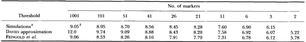
TABLE 1

Thresholds at 5% level for the interval mapping test calculated for a chromosome of 100 cM and different numbers of markers in BC populations

No. of markers

Threshold 1001 101 51 41 26 21 11 6 3 2

Simulations" 9.05' 8.95 8.70 8.56 8.45 8.28 7.60 6.90

DAVIES approximation 12.0 9.74 9.09 8.88 8.43 8.20 7.58 6.15

FEINC~LD el al. 9.06 8.53 8.26 8.16 7.91 7.79 7.31 6.78 6.12 5.78 6.92 6.07 5.22

u From 10,000 replications with population of size 200.

*

Calculated using proposition 2'of'LB.

has asymptotically a standard Gaussian distribution.

p(

x) follows a

x'

with one d.f. under H,. To find an appropriate threshold C =

2

corresponding to a global level a for the test TI = Sup( T 2 ( x ) , 0 5 x 5

p )

where

p

is the length of a single given interval, we have used DAVIES' (1977) bound

a

- = Pr(sup,,,pT(x)

>

c)

2

(2)

1 1 P

=

w-4

+

-

2.R exp(-

2

2 )

I

d

-p,,(x,

p )

dx

[

a'Cov(T(& T(Y))]

where pll (x,

p )

is the autocorrelation function defined bY

PI,(x,

P)

=

aY'

y = x

and @ ( x ) is the cumulative normal distribution func- tion. In the case of BC populations and ignoring double recombination we found (RGM):

I'

d m )

dx = 2 Arctan

0

The problem in generalizing this approach to a chro- mosome is that the derivative of T( x) is not continuous on [ 0 , PI, the discontinuities occurring on the marker positions. DAVIES (1987) observed that approximation

(2) is still appropriate when the derivative has a finite number ofjumps. In regard to this, approximation (2)

could be extended to the chromosome by

The integrals are evaluated for each interval and c cal- culated by successive approximations for a given value of

a. Note that

p i

is not equal to P unless the frequency of double recombination is neglected. The approxima- tion could also be used with distances from any mapping function but we have taken the recombination fraction as the distance (double recombination ignored). Cal- culations based on distances from other mapping func-

tions or taking into account double recombination give similar values. In the case where m is high (number of jumps in the derivative tends to infinity) conditions for the DAVIES' approximation are not well satisfied and other approximations are available.

Other approximations: LB have proved that TI is a

stationary Gaussian process with a covariance function satisfjmg, for any mapping function,

Cov(T(x), T(y)) = R(t) = 1 - 2t

+

o(t') as t + O

where t = I x - yl.

Based on this result LB showed that the threshold for the LOD test for an infinitely dense-map could be ap- proximated by their proposition 2: the threshold C for a genome of H chromosomes and genetic length G (in Morgans) is obtained by solving the equation a = ( H

+

2GC)?( C) where

x2(

.) denotes the inverse cumulative distribution function of the

x'

distribution with 1 d.f. FEINGOLD et al. (1993) proposed another approximation for quite dense maps which is also appropriate in our context. In our case it is:

a = 1 - @(c)

+

2Lcf#)(c)v[2cfl] (4)

where L is the genetic length of the chromosome ex- pressed in Morgans ( L = - 2 ln(1 - 2P) if we use the Haldane (1919) mapping function), $(x) is the prob- ability density function for the standard normal distri- bution,

A

the average marker spacing in cM and v(p) is a special function used by SIEGMUND (1985, p. 82) which can be approximated by v(p) = exp( -0.583~)

+

o(p2).

Results Results for a =

5%

from calculations based on both approximations (3) and (4) with those from simulations (10,000 replications) using the likelihood- based interval mapping method are given in Table 1.

Values of C = c2, the threshold for the test T, are pre- sented for L = 100 CM and various numbers of equi- distant markers. We see that (3) gives the best approxi- mation except for very high marker densities where (4)

is better. This is because approximation (4) performs well when c f i converges to a finite limit so that the argument of v is not extremely large. The DAVIES' a p proximation seems to be appropriate for threshold cal- culations for most experimental marker maps (26 to 3

markers per chromosome) and could be applied even

Threshold of Test for QTL Detection 237

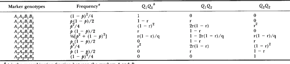
TABLE 2

Marginal and conditional distributions of QTL genotypes given the genotypes of the flanking codominant markers in F, populations

with no double crossing over

Marker genotypes Frequency' Q1 Q1 Q1 Q2 Q 2 4 2

0 0

r 0

2r(l - r) r2

1 - r 0

1 - 2r(l - r)/q - r)/q

1 - r r

2r(l - r) (1 - r)'

r 1 - r

0 1

~~

is the recombination fraction between the markers A and B.

'!is the recombination rate between the putative QTL and the left marker A, r = x/p and q = 1

+

( 1 - l/p)'.

when the markers are not equally spaced. Calculations at the 1% level (results not shown) yield the same con- clusions. Note that our simulations gave values which are different from those of DARVASI et al. (1993) (multiply their values by 217210 = 4.6 to get them on a

2

scale). In fact, for 6 markers they proposed 6.58 and our simu- lations gave 6.9 with [6.73,7.07] as a 95% confidence interval. This is probably due to: first, the difference in size of the population used (200 here against 1000 in DARVASI et a l . ) and second to different likelihood maxi- mization algorithms. DARVASI et al. used a Newton- Raphson algorithm where the derivatives of the likeli- hood function were calculated analytically whereas we used the procedure E04AJF from the NAG li- brary (1990) based on a quasi-Newton algorithm which proceeds numerically and has different convergence criteria.

THE MULTIPARAMETER CASE

General theory: Consider a population of size n and

the corresponding linear regression model Y = X P

+

e

where Y = ( Yl

. . .

Y , )

'

the observation vector, X the

( n , s) incidence matrix of known coefficients depend- ing on the position ( x ) of test on the marker interval considered, /3 the column vector of the s unknown pa- rameters and e the vector of residuals with means 0 and covariance matrix $1. Let X = [ X , I X , ] and /3 =

[Po

I PI]

'

where

PI

is the k vector of the QTL parameters (e.g., additivity and dominance) and

Po

are the vector of other parameters (e.g., general mean). X , is the submatrix (having elements 0 or 1) relative to

Po

and X , the subma- trix corresponding to

PI

which elements depend on x

and are calculated using Table 2. Suppose we are inter- ested in testing H,:

PI

= 0 against

p,

# 0 then the ap- propriate test statistic is (GRAYBILL 1976):

Y ( x x - - X , x ; ) Y

8

T(x) =

where X X - = X ( X ' X ) " X r . When the number of o b servations is large (say 72 2 200) $ could be replaced by

g ,

its linear model estimator, without any modification in the distribution of T ( x) which follows a

x:

under H,.

Let us denote

Q

= X X - - X , X ; and A,,

.

. .

,

A, the non-zero eigenvalues of Q(8QJdx) Q [see DAVIES (1987)

for the underlying theory]. The significance level for T ( x) performed along the entire chromosome could be approximately calculated by:

a = Pr(Sup(T(x)o,,,)

>

C)

= Pr(X:

>

C) ( 5 )

where q j ( j = 1,

. . .

,

k ) are independent centered nor- mal random variables with variances given by the Aj and

11

qll = ( q r q ) ' / ' . DAVIES (1987) used the approximation:

In the case where k = 2 the approximation above be- comes:

where A, 2 A, and

6

denotes a complete elliptic integral of the second kind (ABRAMOWITZ and STEGUN 1972, for-

mula 17.3.3) :

( 8 )

Expressions (6) and

(7)

are due to HARVEY (1965).

t(x) could not be expressed analytically as a function of x but some approximations are available. One of these is (hRAMOWITZ and STEGUN 1972, formula 17.3.35):

a x ) = [I

+

a,z

+

+7?']

+

[biz

+

4zZ]ln(l/z)

+

€(%),€(x)

<

4.10-5 (9)

238 A. Rebai, B. Goffhet and B. Mangin

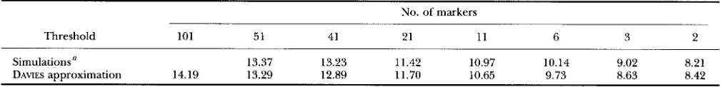
TABLE 3

Thresholds at 5% level for the interval mapping test calculated for a chromosome of 100 cM and different numbers of markers in F, population

No. of markers

Threshold 101 51 41 21 11 6 3 2

Simulations' 13.37 13.23 11.42 10.97 10.14 9.02 8.21 14.19

DAWES approximation 13.29 12.89 11.70 10.65 9.73 8.63 8.42

a From 5,000 replications with population size of 200.

0.24527 and b, = 0.04124.

Alternatively, DAVIES (1987) showed that

and proposed to use the following approximation for the significance level

This formula can be used for approximate simulation- based calculation of the significance value for any ex- perimental design. It is particularly useful when analyti- cal expressions of the eigenvalues could not be obtained.

Application to F, populations: The model for F, populations is described in CARBONELL et al. (1992). Ex- pectations of the genotypic classes for a pair of codomi- nants markers where double recombination is neglected are given in the APPENDIX ( A l ) (based on Table 2). To simplify the evaluation of the eigenvalues we started by computing

A = X i X , , B =

(%)(%),

F = (?)Xl.

These three matrices were found to be diagonal and therefore we just need to compute eigenvalues of

D = A-'B - (A-')'P (11)

as proposed by DAVIES (1987). Expressions for A,, A,,

found after some formal algebra calculations using MAPLE (CHAR et al. 1988), are given in the APPENDIX

(Al). The ratio A = &/A, is always less than 1 and has its maximum value at x = 0 or

p

and its minimum for

x = p/2. Approximation (5) applies here as:

Ir

y L I 1

where f ( r,

p , )

is approximated by

where uj and bj are the constants defined in (9). Calcu-

lations from (12) were done using the eigenvalues found when double recombinations with no interference is as- sumed, which are too complicated to be included in this study. We have written a Fortran

77

program which com- putes, for any given level a! and any set of linked markers

on a chromosome, the threshold for QTL detection test in F, populations when additivity and dominance are considered. Simulations were done using the likelihood approach of interval mapping described by VAN OOIJEN

(1992). The results, given in Table 3, show that the DAVIES' bound is a good approximation to the threshold, especially for marker densities which are customary in QTL mapping experiments (a marker very 5 to 20 cM)

.

Thresholds were also calculated for the 1% level and results (not shown) confirm the good quality of the DAwEs-based approximations. VAN OOIJEN (1992) gave a

value of 11.74 for the threshold at 5% level in F, popu- lation for a chromosome of 120 cM with markers each

5 cM based on 16,000 simulations. Our approximation gives 12.08 which is rather satisfactory.

TOWARD A GENERAL THRESHOLD APPROACH The DAVIES' bound given by formula (5) could be computed for any experimental population and would give good approximations for the thresholds of tests when the population size is not too small ( n 2 200). However formal calculations needed could be difficult to carry out, particularly when three or more parameter are involved as in the case for diallel schemes. If the eigenvalues or the integral (6) could not be directly ex- pressed as a function of x one could use either numerical approximations or expression (10) to carry out easy simulations.

We have studied the situation of F, progenies derived from a diallel cross between four inbreds as described in REBA and GOFFINET (1993). The test T = Y' ( X X - -

T h r e s h o l d of T e s t f o r QTL Detection 239

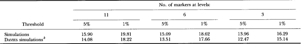
TABLE 4

Thresholds for the interval mapping test calculated for a chromosome of 100 c M with 11,6 and 3 markers in F, populations derived from a diallel cross

No. of markers at levels:

11 6 3

Threshold 5% 1% 5% 1% 5% 1%

Simulations 15.90 19.81 15.09 18.62 13.96 16.29

DAVIES simulations 14.08 18.22 13.51 17.66 12.47 15.14

See text for further details.

’

Based on approximation (10).

old is then the mean, over replications, of C values. Re- sults for the diallel over 1,000 simulations with c? = 1

and a total population size of 600 are shown in Table 4. The deviation between simulated and approximated val- ues is larger than that previously calculated for BC or F,, probably in relation with the small number of replica- tions and individuals (six connected F, populations each with 100 individuals). Nevertheless (10) gives a quite satisfactory approximation and would be very useful when investigating the thresholds for tests in complex crossing designs.

Consider a species having Hchromosomes. To ensure an overall significance level a for the test of QTL over the genome one could take a level ai per chromosome. Traditionally a, are taken all equal: ai = 1 - (1 - a ) l’H.

However ai, the per-chromosome level, could be chosen by a manner which takes into account the relative lengths of all chromosomes. We hope to raise some new issues on this in future work. The level ai, once chosen, is used to compute the corresponding threshold for the QTL detection test by the approach described in this paper.

Fortran 77 programs, using subroutines from the NAG library (1990), which calculate the thresholds for any given level and any distribution of codominant markers on a chromosome for BC, recombinant inbreds and F, populations have been written, compiled and suc- cessfully tested. Note that for recombinant inbreds the same approximation ( 3 ) is used, but there are minor trans- formations to obtain the integral [see APPENDIX

(M)].

For illustration consider the case of a genome with 12 chromosomes each of length 100 cM (similar to the to- mato) and all having markers every 20 cM. To ensure a global significance level of 5% we use a nominal level of 0.5% for each chromosome and found thresholds of 11.64 (2.5 in LOD unit) and 14.65 (3.18) for BC and F, populations, respectively. These values are greater than those classically used for interval mapping (2.4 and 3 ,

respectively). Moreover our method can provide a spe- cific threshold for each chromosome relating to the ac- tual distribution of markers on it. We are happy to make our programs available to interested readers.

We think that the use of the DAMES’ bounds is a good tool to calculate approximate thresholds for interval mapping tests in a wide variety of experimental designs.

This research was partly supported by Rustica semences (Domaine de Sandreau, 31700 Mondonville). w e thank PATRICKVINCOURT for his encouragement in this and other studies. We are grateful to the re- viewers for their helpful comments.

LITERATURE CITED

ABRAMOWITZ, M., and I. A. STEGUN, 1972 Handbook of Mathematical Functions with Formulas, Graphs and Mathematical Tables. Do- ver, New York.

W O N E L L , E. A,, T. M. GERIC, E. BALANSARD and M. J. ASINS, 1992 In- terval mapping in the analysis of nonadditive quantitative trait loci. Biometrics 4 8 305-315.

CHAR, B. W., K. 0. GEDDES, M. B. GONNET, M. B. MONACAN and S. M. WATT, 1988 MAPLE Reference Manual, Ed. 5. Symbolic Com- putation Group, Waterloo, Ontario, Canada.

tecting Marker-QTL linkage and estimating QTL gene effect and map location using a saturated genetic map. Genetics 134: 943-95 1.

DAVIES, R. B., 1977 Hypothesis testing when nuisance parameter is present only under the alternative. Biometrika 6 4 247-254. DAVIES, R. B., 1987 Hypothesis testing when nuisance parameter is

present only under the alternative. Biometrika 74: 33-43. FEINGOLD, E., P. 0. BROWN, and D. SIECMUND, 1993 Gaussian models

for genetic linkage analysis using complete high-resolution maps of identity by descent. Am. J. Hum. Genet. 53: 234-251. HALDANE, J. B. S., 1919 The combination of linkage values and the

calculation of distances between the loci of linked factors. J. Genet. 8: 299-309.

HALDANE, J. B. S., and C. H. WADDINGTON, 1931 Inbreeding and link- age. Genetics 16: 357-374.

HALEY, C. S., and S. A. KNOTT, 1992 A simple regression method for mapping quantitative trait loci in line crosses using flanking mark- ers. Heredity 69: 315-324.

HARVEY, J. R., 1965 Fractional moments of a quadratic form in non-

central normal random variables. Ph.D. Thesis, North Carolina State University, Raleigh, N.C.

JANSEN, R. C., 1992 A general mixture model for mapping quanti- tative trait loci by using molecular markers. Theor. Appl. Genet.

KNAPP, S. J., W. C. BRIDGES and D. BIRKES, 1990 Mapping quantitative

trait loci using molecular marker linkage maps. Theor. Appl. Genet. 79: 583-592.

LANDER, E. S., and D. BOTSTEIN, 1989 Mapping Mendelian factors underlying quantitative traits using RFLP linkage maps. Genetics

LEADBETTER, M. R., G. LINDCREN and H. ROOTZEN, 1983 Extremes and Related Properties of Random Sequences and Processes. Springer, New York.

MARTINEZ, O., and R. N. CURNOW, 1992 Estimating the locations and the sizes of the effects of quantitative trait loci using flanking markers. Theor. Appl. Genet. 85: 480-488.

MOREN~GONZALEZ, J., 1992 Genetic models to estimate additive and non-additive effects of marker-associated QTL using multiple re- gression techniques. Theor. Appl. Genet. 85: 435-444.

NUMEFXAL ALGORITHMS GROUP, 1990 The NAG Fortran L i b r a 9 Manual-Mark 14. NAG Ltd., Oxford.

DARVASI, B., A. WEIREB, V. MINKE, J. I. WELLER and M. SOLLER, 1993 De-

85: 252-260.

240 A. Rebai, B. Gofinet and B. Mangin

R E B A ~ , A., and B. GOFFINET, 1993 Power of tests for QTL detection SIEGMUND, D., 1985 Sequential analysis: tests and confidence inter-

VAN OOIJEN,J. W., 1992 Accuracy of mapping quantitative trait loci in using replicated progenies derived from a diallel cross. Theor. uals. Springer, New York.

Appl. Genet. 8 6 1014-1022.

R E B A I , A., B. GOFFINET and B. MANGIN, 1994 Comparing power of different methods for QTL detection. Biometrics ( i n

p r e s s ) . Communicating editor: B. S. WEIR

autogamous species. Theor. Appl. Genet. 8 4 : 803-811.

APPENDIX

Al: The linear model for F, populations is Y = Xp

+

e, where /3 = ( p , a , d ) and

p,

= ( a , d ) I . The reduced form

of X is (Table 2) :

1 1 1 1 1 1

0 r 2 4 1 - r ) 1 - r s I - r 2 4 1 - r ) r 0

where r = x/p, s = (1 - 2r

+

2r2)/( 1 - (1 -

l/p)').

In this case the vector of residuals e has variance matrix d V ,

where V-' is a 9 X 9 diagonal matrix whose elements are the expected individual numbers in the nine marker classes (see Table 2). We then have, taking u* = 1,

Q

= v-'(x(X

V " x ) - ' X

- X,(X',

v-~x,)-~x',)v-~.

Unfortunately calculations based on this expression of Q are too complicated. We then used an approximation which consists of working with a centered model Z = X,p

+

e with Z = Y - X,,&,, where

o,,

is the least square estimator

of

p,

from the full model. So one can use

Q =

v-'(x,(x',v-'x,)-'x',)v-'.

We then verified that A = X;V"X,, B = (dXl/ax)V"(dX,/dx) and F = (dX;/dx)V-IX, are all diagonal and used ( 1 1 ) to derive eigenvalues. We found

-4(p'

+

(1 -

p)')(a,

+

a , r + (I2?

+

4 2 r 3 - r4)

A, =

(6,

+

6, r

+ h2?

+

q?(2r3 - r4))'

a , = - 1 + 2 p - p " 3 p 3 + 2 p 4

4,

= 2 - 6p

+

8p2 - 3p3

a, = 4p(2 - 6p

+

9p' - 4p3) 6, = -4(1 - 3p

+

4p' -

p3)

4PU -

P)

(1 - 4pr

+

4@)2

.

A, =

A!& For recombinant inbred lines produced by successive selfings, the recombination between two markers is

R = 2r/ ( 1

+

2r) where r is the actual recombination rate (HALDANE and WADDINGTON 1931). Substituting x and

p

by their respective transforms 2t/(l

+

2t) in the covariance function of the BC (REBA] et al. 1994) leads to

Cov(T(x), T(y)) =

p(l

- 2x - 2y

+

4xy)

+

8xy

2/(p(l

- 2.)'

+

8G')(p(l - 2 ~ ) '

+

8 ~ ' )

and

8P

P I 1 (x3

P)

=

-(p(

1 - Zx)9 + 82)' .