Modeling interference in genetic recombination.

Copyright 0 1995 by the Genetics Society of America

Modeling Interference

in

Genetic Recombination

Mary

Sara

McPeek and

Terence P. Speed

Department of Statistics, University of Calijornia, Berkeley, Calijornin 94720 Manuscript received December 17, 1993

Accepted for publication October 25, 1994

ABSTRACT

In analyzing genetic linkage data it is common to assume that the locations of crossovers along a

chromosome follow a Poisson process, whereas it has long been known that this assumption does not fit the data. In many organisms it appears that the presence of a crossover inhibits the formation of another nearby, a phenomenon known as “interference.” We discuss several point process models for recombination that incorporate position interference but assume no chromatid interference. Using stochastic simulation, we are able to fit the models to a multilocus Drosophila dataset by the method of maximum iikelihood. We find that some biologically inspired point process models incorporating

one or two additional parameters provide a dramatically better fit to the data than the usual “no- interference” Poisson model.

T

HE phenomenon of interference in genetic recom- bination was noticed very early this century by Dro-

sophila melanogaster geneticists in THOMAS HUNT MOR-

GAN’S lab (STURTEVANT 1915; MULLER 1916). They

found that simultaneous recombination in two or three nearby chromosomal intervals occurred much less of- ten than would be expected under independence, and that the effect appeared to decrease with distance. At

present the biological nature of genetic interference is still not well understood, nor has it been adequately modeled mathematically. Virtually all multilocus link- age analyses use the assumption of no interference. Although this assumption may give consistent results for locus ordering (SPEED et al. 1992) and estimation of recombination fractions in some cases, it clearly does not fit the data. It is natural to ask if such an analysis could be improved by the use of a reasonable interfer- ence model. What is required is a biologically plausible point process model for crossovers along a chromo- some, which should be fit to data. The Drosophila data- set of MORGAN et al. (1935) is ideal for this purpose. Previous attempts to fit a crossover point process to the

MORGAN et al. ( 1935) Drosophila dataset ( COBBS 1978;

&SCH and LANGE 1983; PASCOE and MORTON 1987;

GOLDGAR and FAIN 1988; FOSS et al. 1993) have been severely limited by the difficulty of calculating the likeli- hood of the data under all but the simplest models. Using a Monte Carlo method, we are able to fit a wide range of point process models to the data.

BACKGROUND

In diploid eukaryotes, crossing over takes place dur- ing the pachytene phase of meiosis, when the two ho-

Corresponding author: Mary Sara McPeek, Department of Mathemat-

ics, University of Southern California, Los Angeles, CA 90089-1 113. E-mail: [email protected]

Genetics 139: 1031-1044 (February, 1995)

mologous versions of any particular chromosome have each been duplicated and all four resulting strands or chromatids are lined up together, forming a very tight bundle. We model crossovers as being points located along this bundle, and each crossover involves exactly

two of the four chromatids. We assume that the two chromatids involved in any particular crossover are non- sister chromatids, that is, the two chromatids cannot be the two copies of a single homologous chromosome. After crossing over has occurred, the four resulting chromatids are mixtures of the original parental types. In Drosophila, for each meiosis, we will have informa- tion on only one of these four resulting chromatids. If that chromatid was involved in an odd number of crossovers between two loci, a recombination is said to have taken place between the two loci.

It is important to keep in mind that crossing over takes place among four chromatids. In that case the two aspects relevant to recombination are the distribu- tion of crossovers along the bundle of four chromatids and which pair of nonsister chromatids is involved in each crossover. The concept of interference is usually divided into two parts, corresponding to these two as- pects. First, we say that there is position or chiasma interference if the number and location of crossovers in a given region are not independent of the numbers and locations of crossovers in disjoint regions. Second, we say there is chromatid interference if it is not the case that each pair of nonsister chromatids is equally likely to be involved in a crossover, independent of which were involved in other crossovers. There is little consistent evidence of chromatid interference (ZHAO et al. 1995b).

the occurrence of crossovers along the chromosome. In the case of no chromatid interference, the point pro- cess on the single chromatid can be obtained from the point process on the bundle of four by independently thinning ( L e . , deleting) each point with probability This is because the given chromatid has chance of being involved in a particular crossover, indepen- dent of involvement in any others. As a result of assum- ing no chromatid interference, the chance of recombi- nation across an interval increases monotonically as the interval is enlarged, with an upper bound of

The traditional measure of interference is the coinci- dence ( STURTEVANT 1915; MULLER 1916), which is ex- pressed as a ratio. The numerator is the chance of simul- taneous recombination across both of two disjoint intervals on the chromosome. The denominator is the product of the marginal probabilities of recombination across the intervals.

r1 I C =

+

T11) (To1

+

T I , ) ’

where C is the coincidence and rq is the chance of i recombinations across the first interval and

j

recombi- nations across the second interval. If there were no position interference, the coincidence would equal one. Observed coincidences tend to be near zero for small, closely-linked intervals, increasing to one for more distant intervals.

The recombination point processes considered here are stationary in terms of some distance metric, al- though this distance metric is generally not equivalent to physical distance. This point will be discussed further below. For each of the point process models considered here, there is more than one such choice of a distance metric that will make the process stationary; these met- rics are the same up to a multiplicative constant. The genetic distance associated with a chromosome interval is defined to be the expected number of crossovers occurring on a single chromatid within that interval. The metrics in which the models discussed here are stationary are all constant multiples of genetic distance. We shall choose one for notational convenience and call it the stationary metric. Among other things sta- tionarity of the model means that coincidence will be a function of the distances across each of the two intervals considered and the distance between the intervals (in terms of the stationary metric) but not their actual loca- tions. This also implies that the intensity, p = limlb+ h”

Pr (at least 1 point in [ t , t

+

h ) )

,

where his measured in terms of the stationary metric, is the same for all t . Furthermore, for the models considered here the con- ditional intensity can be defined by p ( z ) = limb+o limf+,

E - ’ Pr (at least 1 point in [ t

+

z, t

+

z

+

E )

I

at least 1 point in [ t , t

+

6)

) , where E is measured in terms of

the stationary metric. Intuitively, this is the intensity at

t

+

z conditional on a point at t , and by stationarity this depends only on z. When the conditional intensity exists, the coincidence function can be defined as the coincidence between two intervals, in the limit when the stationary widths of the intervals are allowed to go to zero, as a function of the stationary distance between the two intervals. The coincidence function is given by the ratio of the conditional intensity to the uncondi- tional intensity

C(z)

=

-.

P ( z)

P

Formulae of this type appear in FOSS et al. (1993) and LANDE and STAHL (1993). Note that coincidence is not a complete description of interference but measures interference only between pairs of intervals.

Mdtilocus linkage analysis: When one has a panel of genetic markers, one may be interested in making a linkage map, that is, in ordering the markers and calculating genetic distances between them. Alterna- tively, one may be interested in using linkage analysis to locate a new marker or gene of interest on a previously determined marker map. In both cases the most infor- mative kind of analysis is multilocus linkage analysis, in which one considers recombination patterns among all the marker loci simultaneously.

The Drosophila dataset of MORGAN et al. ( 1935) con- sists of counts of recombination events among nine marker loci on the Xchromosome. The nine loci under consideration are scute, echinus, crossveinless, cut, vermil- ion, sable, forked, carnation and bobbed, and they corre- spond to observed fly phenotypes. The actual positions of the loci on the X chromosome are assumed to be fixed but unknown, and counts of recombination events are made based on the observed physical characteristics of the fly, which are associated with alleles at the nine loci. In Drosophila melanoguster recombination occurs only in females. Consider the X chromosome inherited by a fly from its mother. This X chromosome will be some mixture of the two maternal grandparental X

chromosomes because of crossing over between them. For each of the nine loci, it can be determined whether the offspring fly inherited its maternal grandmother or maternal grandfather’s allele at that locus. Thus, there are possible observed outcomes. However, each out- come has a complementary outcome that is considered equivalent, in terms of recombination, namely the one in which all the grandmaternal and grandpaternal al- leles are switched. Therefore, there are 2’ possible re- combination outcomes, and the number of times each occurs out of 16,136 meioses is recorded in the MORGAN

et al. dataset.

Modeling Interference 1033

recombination in each interval A, for which

x,

= 1, and no recombination in each interval A, for which x, = 0. Then each of the 2’ possible recombination outcomes would correspond to one of the Z 8 possible x’s.

In what follows we assume the order of the loci to be known. If the order were not known, the procedures described below could be repeated for each of a small number of candidate orders, and the estimated order would be the one whose maximized likelihood was high- est. We assume that each event

x

occurs with some fixed probability

p,.

These events correspond to what is o b

served in the data. For each x, we wish to calculate its

probability

p,

under each of the point process models we consider in order to fit the models to the data by maximum likelihood.

Recall that event x occurs when a given chromatid is involved in an odd number of crossovers in each of the intervals Ai for which

xi

= 1 and an even number of

crossovers in each of the intervals A, for which xI = 0.

A set of related events will be denoted y = ( yl ,

. . .

,

y8) ,

yj

= 0 or 1, j = 1,

. . .

,

8. y is the event that, on the bundle of four chromatids, at least one crossover occurs in each of the intervals A, for which

yl

= 1 and no crossovers occur in each of the intervals A, for which

yi

= 0. Note that y is an event occurring on the bundle

of four chromatids, whereas x refers to just one of the four chromatids. We let qv denote the probability of the event y. The assumption of no chromatid interference gives a correspondence between these two sets of proba- bilities ( WEINSTEIN 1936) , namely

1

p,

=

C

qr for all x,

y : l z y 2 x

and inverting,

qy

= 2 y “

x

(-1)

(x-Y)’lpx

for all y,

x : l z - x 2 y

where, for example, y * 1 =

yj,

and 1 2

y

2 xmeans 1 2 y, 2

x,

for all j . Thus, to get the recombination

probabilities under different point process models, as- suming no chromatid interference, it would suffice to calculate probabilities for the simpler events,

y,

corre- sponding to zero or nonzero crossovers in the locus intervals, on the bundle of four chromatids. Once we can calculate the

qv’s

in terms of the unknown parame- ters and from these, the p,’s, we write down the log- likelihood as

constant

+

a, log

( p , ) ,

x

where x = (x,,

. . .

, % ) , xj = 0 or 1, a, is the number of times the event x occurs in the data and where the constant is irrelevant because it does not involve the unknown parameters. We would then maximize the likelihood over the unknown parameters.

MODELS

It is sometimes assumed that the problem of model- ing interference is equivalent to that of formulating a map function, i.e., a function from [ O , a) to

[ o ,

1/2]

that maps expected number of crossovers to chance of a recombination. This is not the case. First, a map func- tion is not a full-fledged model. By itself, a map function does not provide probabilities for multilocus recombi- nation events when more than three loci are involved, and so it cannot be fit to data such as that described above. In an attempt to remedy this problem, LIBERMAN and KARLIN ( 1984) introduced multilocus map func- tions, which are defined as above, but with the addi- tional property that the map function relationship be- tween expected number of crossovers and chance of a recombination should hold on unions of disjoint inter- vals, as well as on intervals. Unfortunately, these multilo- cus map functions correspond to an extremely limited class of models under the assumption of no chromatid interference. EVANS et al. (1992) showed that under this assumption the only models that have multilocus map functions are the count-location models described by KARLIN and LIBERMAN ( 1979) and RISCH and LANCE

( 1979). These models have the undesirable property that the coincidence function is constant, ie., the level of interference, as measured by coincidence does not vary at all with the genetic distance between the inter- vals considered. In actual data coincidence seems to be close to zero for near intervals and close to one for more distant intervals (see Figure 2 ) . For this reason the count-location model does not appear well suited to modeling interference. It is, however, easy to fit and has been previously fit to the Drosophila data of

MOR-

GAN et al. ( RISCH and LANGE, 1983)

.

We include it here for comparison. The model will be described in more detail below.

Poisson model: COX and ISHAM ( 1980) provide an introduction to point processes. The simplest crossover point process model we consider is the Poisson process. This model was proposed for recombination by HAL-

DANE (1919) and continues to be virtually the only model used in linkage analysis. The model allows no interference at all, i.e., crossing over in disjoint intervals is independent, or the presence of one crossover does not alter the chance of others occurring nearby. Thus, the coincidence function has the constant value 1. In the general formulation of the Poisson model, we let pt denote the intensity of the process at physical location t

along the bundle of four chromatids, i.e.,

P

(at least 1 point in ( t , t

+

h ] )

pI = lim

h-0 h

P.

of no crossovers in a given interval [ a , b ) is exp (

-J%

p , d t ) , or in . the homogeneous case where pL = p for all t . To get the probability of a given event y , i.e.,

the event of at least one crossover in each interval for which

y,

= 1 and no crossovers in each interval for which yi = 0, we multiply the appropriate probabilities for each interval using independence.

If we let 11,

.

. . ,

4)

denote the physical locations of the nine marker loci, then from recombination data the estimable quantities in the Poisson model are the genetic distances ( i e . , expected numbers of crossovers on a single chromatid) between the markers, namely,

(The factor of occurs because each crossover on the bundle of four chromatids is assumed to involve a given chromatid with chance Thus, from the data one cannot infer anything about possible inhomogene- ity of the Poisson intensity, because this cannot be sepa- rated from the unknown locations of the marker loci. Similarly, one cannot estimate the actual locations of the markers nor the physical distances between them. Associating the interval [ 0, 11 on the real line with the chromosomal segment between the outermost loci under consideration and letting p, and 0 = lI

<

<

4)

= 1 be as before, let p =

si,

p,dt and M ( z ) = p"

st)

p,dt, for all z E [0, 11. Then M : [ 0, 11 "f [ O , 11 is

monotone nondecreasing and onto ( i.~., for every point u~ E [ 0,1] there is some z E [ 0,1] such that w = M ( z ) ) ,

hence continuous. M can be thought of as a continuous cumulative distribution function (cdf) on [ 0, I ] . If we transform each point of the Poisson process by A 4 , then the resulting process is homogeneous Poisson with inten- sity p. The transformed homogeneous process on [ 0, 11

with marker locations M ( lI )

<

-

<

M (

4 ) )

and the original inhomogeneous process on [O, 13 with marker locations lI

<

<

4,

would both produce recombina- tion data with the same distribution. Thus, without loss of generality, we may consider only homogeneous Poisson processes, that is, we let p, = p for all t . The estimable parameters of the model are the genetic distances, d l ,

. .

.

, &, between the markers, and in terms of these the probability of the event y is

x

n

e-2112?, ( 1 - e - 2 d , ) (I-?,)

, = I

Note that p can be written in terms of this parametriza- tion: p = 2 E:=, d , .

Gamma model: The distances between crossovers in the homogeneous Poisson model are independent ex-

ponential random variables, or equivalently, gamma with shape parameter 1. One way to generalize the Pois- son model would be to consider renewal processes with general gamma interarrivals, thus adding an extra pa- rameter to the model. On the real line the stationary renewal process with gamma interarrivals can be formu- lated as follows. Given a point at location w, the density of the distance to the next point to the right is

where Istands for interarrival,

r(

y ) =

J;;"

pysy" p P v ' ds 9

and this is independent of the occurrence of any points to the left of 7u. The distribution of the next point to the left of w is the same; there is no directionality. The distribution of the distance to the first point to the right ( o r equivalently left) of 7u, when it is not assumed that a point has occurred at zu, has density

The intensity of the process is then p / y . Letting y =

1, we would get the Poisson model. The coincidence function for the gamma model is

r

C ( z ) =

1

f ; ' ( z ) ,

P n = l

where f ( z ) = l-( y n ) " p y 7 ' z y 7 ' " ~ p v z .

We associate the interval [ 0, 11 with the bundle of four chromatids, and we consider the above process restricted to [ 0, 11

.

Then the chance of at least one crossover occurring on the bundle of four chromatids is a =

s

,f; ,( ( z ) dz, and given that at least one crossover

occurs, the density of the distance from the 0 end of the bundle to the first crossover is a - I f , , , ( z )

.

Given a

crossover at location w E [ 0, 11, the chance that an- other crossover occurs between w and 1 is @ ( w) =

sb7'f,(

z ) d z . Given a crossover at location 7u, and given that at least one crossover occurs between w and 1, the density of the distance from w to the next crossover between wand 1 is @ (

w)

"A(

z )

.

Note that all distances are in terms of a metric whose relationship with physical distance is unknown but which is a constant multiple of genetic distance.

We consider the gamma model on the bundle of four chromatids, and the points are then independently thinned, each with chance ( Z.C., each point has

Modeling Interference 1035

the crossover point process along a single chromatid be viewed as a renewal process with interarrival density

f

( z )

= '/*T sech ( '/*Tz) tanh ( '/*7rz). OWEN (1949, 1950) found that a gamma interarrival density with shape pa- rameter 2 and scale parameter 2 was mathematically trac- table and closely approximated the renewal process pro- posed by FISHER et al. CARTER and ROBERTSON (1952) used the gamma with shape parameter 2 as a four-strand model and applied various models of chromatid interfer- ence to get the chance of recombination across an inter- val for a single chromatid. PAYNE ( 1956) considered the gamma with integer shape parameter as a twestrand model. He compared coincidence curves for the gammas with shapes 2 and 3 to data. COBBS ( 1978) considered the gamma with integer shape parameter as a four-strand model, assuming no chromatid interference. He fit the model to Neurospora and Drosophila data by comparing the observed distribution of the number of crossovers in a segment (ignoring those that could not be observed) to the number predicted by the model. STAM (1979) considered various mathematical aspects of the same model, and Foss et al. ( 1993) also considered this model, comparing the coincidence curves from the model to coincidence curves for Drosophila and Neurospora data. In this paper we calculate approximate probabilities of the different possible multilocus recombination events under the model, and we fit the model to the data by maximum likelihood. We are able to compare observed to expected frequencies of recombination events. This subsumes both the comparisons of distributions of num- ber of events and of coincidence curves.

The gamma interarrival process with integer shape parameter has been used in the literature so often largely because of relative mathematical tractability. However, FOSS et al. ( 1993) propose it to explain cer- tain empirical observations concerning recombination and gene conversion ( a nonreciprocal exchange of ge- netic material between homologous chromosomes). First, gene conversion is associated with a high fre- quency of recombination of flanking markers ( MORTI-

MER and FOGEL 1974). Second, gene conversions seem to occur independently in disjoint intervals, but gene conversions accompanied by recombination do not; rather, they appear to inhibit each other (

MORTIMER

and FOGEL 1974). The model proposed by Foss et al.

(see also STAHL 1979; MORTIMER and FOGEL 1974) is that initial precrossover events occur along the chromo- some according to a Poisson process. Each such event results in a gene conversion and may or may not result in a crossover as well. Their model holds that every ( m

+

1 ) st initial event results in a crossover. If the first event has chance 1

/

( m

+

1) to form a crossover, then the model is equivalent to the stationary gamma interar- rival model with shape parameter m

+

1.

We note that, as in the case of the Poisson model, if

we fit the stationary gamma renewal process, we are also allowing for the possibility that the true physical process may be nonstationary. The class of models cov- ered by the analysis consists of those for which a mono- tone nondecreasing onto transformation M [ 0 , 13 -+

[ 0 , 13 (i.e., a continuous, cdf on [ 0 , 13 ) exists that maps the model to a stationary model. The models corresponding to almosteverywhere differentiable M ' s

are those that can be formulated as follows. Given a

point at w , the density of the distance to the first point to the right of w is

where p t = p X d M ( t )

/

dt. The density of the distance to the first point to the right of a given location w , when it is not assumed that a point has occurred at w , is

The intensity of the process at location t is y - ' p r . Note that the coincidence function is identical to that for the stationary case.

The estimable parameters are the shape parameter

y and the genetic distances d l ,

. .

.

,

4 .

Note that p can be written, in terms of this parametrization, as p = 2 y

X:=l

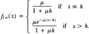
d , . It has not proved possible to write down an explicit expression for the likelihood of the data under the gamma model, except in the case of integer-shape parameter (ZHAO et al. 1995a). Instead, the likelihood has been simulated, as described below.

Hard-core model: Another generalization of the Poisson model would be to have the points follow a Poisson process but with no two points allowed to be closer than a certain fixed distance h. This is known as a hard-core model (see e.g., STOYAN et al. 1987). On the real line this is just a stationary renewal process with interarrivals distributed as exponential plus a constant. That is, given a point at location w , the distance to the next point to the right (equivalently, left) has density

p e - p L ( z - h ) for z

>

h

0 otherwise.

=

The distribution of the distance to the first point to the right (equivalently, left) of w , when it is not assumed that a point has occurred at w , has density

K h if z s h

= 0, we would get the Poisson model. The coincidence function for the hard-core model is

m

where

Again, we associate the interval [ 0,1] with the bundle of four chromatids. The restriction of this stationary renewal process to the interval [0, 11 works exactly as in the gamma case. As before, this hard-core model is equivalent, in terms of the data, to any model resulting from a transformation of the interval by a continuous cdf M . The models corresponding to almost-everywhere differentiable M’s are those that can be formulated as follows. Given a point at w , the density of the distance to the first point to the right of w is

( 0 otherwise,

whe;se, = p X d M ( t )

/

dt, and h,

>

0 is any solution of

s,

pSds =

B ,

where B = hp. The density of the distance to the first point to the right of a given location w , when it is not assumed that a point has occurred at w . is

The intensity of the process at location tis p l / (1

+

B)

.

The estimable parameters are the hard-core genetic distance, hg = 1/2 B/ ( 1

+

B ) , and the genetic distances

between the points, dl, .

. .

,

&.

Note that p can be expressed in terms of this parametrization as p = (1 -

2 4 ) ”

X:=l

d,. As the number of loci increases, the likelihood quickly becomes very complicated, and no tractable general form has been found.

King-Mower model: In one version of a model sug- gested by KING and MORTIMER (1990), points are put down on a segment of the real line according to a Pois- son process with parameter p, just as in the original stationary Poisson model described above. Starting from time 0, each point independently waits an expo- nential amount of time with parameter h before starting polymer growth, i.e., the density of the time to polymer growth is f( t ) = l e - ” . When a polymer starts to grow from a point, it grows in both directions at a constant rate g. If a polymer from one point hits another point that has not yet started to grow, the latter point is de- leted. At first glance this process appears to be nearly

identical to the one-dimensional version of the John- son-Mehl model (JOHNSON and MEHL 1939, but MEIJER-

ING 1953 is more readable) for random tessellations. In that model points are born over time and immedi- ately start growing polymers (called “crystals” byJOHN- SON and MEHL 1939) at rate g in both directions. In the Johnson-Mehl model the rate of birth in an unpoly- merized interval [ w , w

+

h , ) during an interval of time

[ t , t

+

b)

is p h l b

+

o ( h l b ) . That is, in any infinitesi- mal interval of time [ t , t

+

b)

,

it is a Poisson process, with parameter p b , on the unpolymerized part of the line. In any small unpolymerized interval [ w , UI

+

h,)

along the line, one waits an exponential amount of time, with parameter phi, for a point to appear and start growing. However, in the King-Mortimer model the chance that a polymer starts to grow in a small unpolymerized interval [ w , w

+

h,) during an interval of time [ t , t

+

b)

can be shown to be phe-“h11~2

+

o ( h , & ) , ie . , it varies over time, going monotonically to zero.

In the King-Mortimer model there is an initial Pois- son distribution of points, then the polymerizing pro- cess takes place over time, and then there is some re- sulting final distribution of points. Intuitively, it is clear that the final distribution of points would not be af- fected if time were slowed down or speeded up by some constant multiple c, as long as the initial Poisson distri- bution of points remained the same. This would be equivalent to changing h to A and changing g to cg.

Therefore, it is not surprising that the final distribution of points is determined by p and g / X only. Thus, with- out loss of generality, we may take A = 1.

KING and MORTIMER ( 1990) choose parameter values for which their simulations appear to resemble ob- served data, but they do not actually fit the model. They consider the process as defined on a line segment. In that case points are more likely to occur near the ends of the segment, because there are no points outside the segment to interfere with them. This is also true in the case of the hard-core model defined on a segment. We instead consider the process as defined on the real line and then restricted to [ 0, 11. In that case the points near the ends of the segment behave as if other points lying outside the segment could interfere with them, and the model is stationary. As before, a nonstationary model resulting from a transformation of the interval [ 0, 13 by a continuous cdf M is indistinguishable, in terms of the data, from the stationary model. This non- stationarity is of a different type from that introduced by considering the process only on an interval, as KING and MORTIMER (1990) have done. The nonstationary models with almost-everywhere differentiable M’s COV- ered by this analysis are those in which the initial Pois- son distribution has inhomogeneous parameter /.L~ =

Modeling Interference 1037

reached position t i s gt = g d M ( t )

/

dt. We note that the stationary process is not a renewal process; given a point at w E [ 0, 11, the distribution of the distance to the next point to the right of w is not independent of the occurrence of other points to the left of w .

To specify the stationary King-Mortimer model on [ 0, 11

,

it is convenient to determine the distribution of the time when a polymer growing from somewhere outside [ 0, 11 would reach that interval. To do this, we ignore, for the moment, points inside [ 0, 11 that could potentially polymerize and prevent any outside poly- mers from ever reaching [ 0, 11

.

To calculate the distri- bution of the time when a polymer from ( 1, a) reaches

1, we let X,, for each i

>

1, be the distance between the ith and ( i - 1 ) st initial points to the right of 1. If

XI is the distance from 1 to the first initial point to the right of 1, then the

X,

are independent exponential( p )

.

Let Z, be the waiting time for polymer growth of the ith initial point to the right of 1. The Z, are independent exponential( 1 ) . Let S, = g"

Z;=l

X,.

Then the chance that no polymer arrives at 1 from the right before time t is

P(S1

>

t )

cc

+

P ( S , 5 t

<

S,

+

5

>

t , for a l I j 5 2).

1 = 1

The ith term of the sum is found to be

and so the required probability is

e'lg( 1 - l - C O

One minus this quantity is the cdf of the time that a polymer first arrives from the right (equivalently, left) at any given point. This cdf is useful for simulating the process. Substituting 2g in for g gives the cdf of the time that a polymer first arrives at any given point from either the right or the left, ignoring the possibility that the point itself grows first and prevents the polymer's arrival. From this we can calculate the intensity of the point process, which isjust the intensity, y , of the initial Poisson process multiplied by the chance that a given initial point starts to grow before another polymer ar- rives. This is

where a = 2pg and

r(

x, y ) =

Sh

t"" e-'dt, known as the incomplete gamma function. The estimable param- eters under this version of the King-Mortimer model are the genetic distances, d l ,

. .

.

,

&,

and the expected time for a polymer to traverse the distance between

two adjacent points in the initial Poisson process, as a multiple of expected waiting time for a polymer to start growing: T = ( y g )

-'

= 2 6 ' . Note that y can be ex- pressed in terms of this parametrization:

No closed-form expression is known for the likelihood of recombination data under this model, nor for the coincidence function. Both of these are obtained here by simulation.

K-M 11 model: The second King-Mortimer model ( K I N G and MORTIMER 1990), which shall be called here

K-M 11, is the same as the previous model except that a parameter is added for termination of polymer growth, once it has started. That is, under the set-up of the previous model, each polymer now grows for an inde- pendent exponential( 1 / v ) amount of time, or until it hits another polymer, whichever happens first. The possibility of early termination of a polymer has the effect of allowing interference to operate over a smaller range than before. Interference can then be made more intense, yet more localized, than in the ordinary King-Mortimer model. For this model there is no known expression for the intensity, the likelihood of recombination data nor for the coincidence function. The parameters estimated are the genetic distances, d l ,

.

.

.

,

4 ,

the expected time for a polymer to traverse the distance between two adjacent points in the initial Poisson configuration (given that growth does not ter- minate up to that time) , T , and the expected time to terminate polymer growth, v , where each of these times is expressed as a multiple of the expected waiting time for a polymer to start growing.

Count-location model: In the count-location model (KARLIN and LIBERMAN 1979, called the "generalized no interference model" by RISCH and LANCE 1979) the number of crossovers is chosen according to some count distribution c, where c is given by k, cl

,

. .

.

, and

c, = P ( i crossovers). Given the number of crossovers,

their locations are independent and identically distrib- uted (i.i.d.) along the bundle of chromatids, according to a location distribution

v

that does not vary with the count. The count-location model can be thought of as a modification of the Poisson process model, in which the number of crossovers occurring is no longer Pois- son, but their locations are again i.i.d. as in the Poisson model. In the count-location model the coincidence function is constant:

n

C ( z ) = i ( i - l ) c ,

/(

i

i q .

* = 2 j = 1

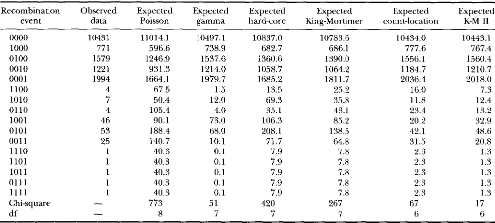
TABLE 1

Observed and expected counts under the fitted models for five loci with chi-square statistics

Recombination Observed Expected Expected Expected Expected Expected Expected

event data Poisson gamma hardcore King-Mortimer count-location K-M I1

0000 10431 11014.1 10497.1 10837.0 10783.6 10434.0 10443.1

1000 771 596.6 738.9 682.7 686.1 777.6 767.4

0100 1579 1246.9 1537.6 1360.6 1390.0 1556.1 1560.4

0010 1221 931.3 1214.0 1058.7 1064.2 1184.7 1210.7

0001 1994 1664.1 1979.7 1685.2 1811.7 2036.4 2018.0

1100 4 67.5 1.5 13.5 25.2 16.0 7.3

1010 7 50.4 12.0 69.3 35.8 11.8 12.4

01 10 4 105.4 4.0 35.1 43.1 23.4 13.2

1001 46 90.1 73.0 106.3 85.2 20.2 32.9

0101 53 188.4 68.0 208.1 138.5 42.1 48.6

001 1 25 140.7 10.1 71.7 64.8 31.5 20.8

1110 1 40.3 0.1 7.9 7.8 2.3 1.3

1101 1 40.3 0.1 7.9 7.8 2.3 1 .3

101 1 1 40.3 0.1 7.9 7.8 2.3 1.3

0111 1 40.3 0.1 7.9 7.8 2.3 1.3

1111 1 40.3 0.1 7.9 7.8 2.3 1.3

Chi-square

-

773 51 420 267 67 17

df

-

8 7 7 7 6 6

Triple and quadruple recombination events are quite rate. These events were pooled in the analysis because accurate probabili- ties for the events could not be computed by simulation.

simultaneously, i.e., c, = 1 and cj = 0 for i

>

3. The location distribution v may be taken to be uniform without loss of generality, because the class of models covered by this analysis will include all those with loca- tion distributions having a continuous cdf. The intensity of the process is

Z:,,

ic,

.

The model can be parame- trized in terms of the genetic distances, dl,

. . .

,

&,

and q, and cl. The likelihood can be calculated explicitly in terms of these parameters.

To fit any of these models to recombination data, it is necessary to be able to calculate qr for any y , that is, the probability of any combination of zero and nonzero crossover counts in the eight marker intervals, as de- scribed above. This is trivial for the Poisson model and the count-location model. For the other models this involves integrating the density over all possible realiza- tions compatible with y , assuming that the density is known or can be computed. So far, these integrals ap- pear virtually impossible to do exactly, except in the special case of gamma with integer shape parameter.

As a result, they have been calculated here by Monte Carlo methods. For the Poisson, gamma, count-location and K-M I1 models, the recombination probabilities were computed for events among all nine loci, whereas for the other models only a subset of five of the nine loci were used.

For a given model the probability qr depends not only on the model parameters but also on the relative locations of the loci. For each choice of model parame- ters, a large number n of realizations of the point pro-

cess are simulated. Using these simulations, the desired probability qr can be estimated, for any set of locus locations, by the observed frequency of the event y.

From the q's the estimates of the probabilities of the observed recombination events can be computed, and from these, the estimated likelihood of the observed data is computed. Recombination events in which three or more recombinations took place were so rare in this data that their probabilities are very difficult to esti- mate. These rare events were pooled in this analysis. Holding the point process parameters fixed, the likeli- hood can then be numerically maximized over the locus locations by the Nelder-Mead search algorithm

( NELDER and MEAD 1965). This maximization is done

TABLE 2

Fitted point process parameters for five loci

Model Parameter(s) ''

Gamma y = 6.41 (0.280)

Hard-core hK = 0.116 (0.004)

King-Mortimer I T = 0.038 (0.005)

Count-location q, = 0.311 (0.005), c, = 0.641 (0.007) (redundant parameters: G> =

0.0448 (0.005), CS = 0.0032

(0.002))

0.244 (0.187)

K-M I1 T = 1.01 X (2.44 X =

Modeling Interference

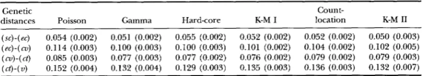
TABLE 3

Fitted genetic distances between adjacent markers for five loci

1039

Genetic Count-

distances Poisson Gamma Hard-core K-M I location K-M I1

( x ) - ( e c ) 0.054 (0.002) 0.051 (0.002) 0.055 (0.002) 0.052 (0.002) 0.052 (0.002) 0.050 (0.003) (ec)-(cu) 0.114 (0.003) 0.100 (0.003) 0.100 (0.003) 0.101 (0.002) 0.104 (0.002) 0.102 (0.005)

( a ) - ( c t ) 0.085 (0.003) 0.077 (0.003) 0.077 (0.002) 0.076 (0.002) 0.079 (0.002) 0.079 (0.003)

( c t ) - ( v ) 0.152 (0.004) 0.132 (0.004) 0.129 (0.003) 0.135 (0.003) 0.136 (0.003) 0.132 (0.007)

Estimated standard deviations in parentheses.

using the same set of n simulated realizations. For each choice of model parameters, the process can be re- peated, generating a new set of n realizations and max- imizing the estimated likelihood over the locus loca- tions. The Nelder-Mead search algorithm can then be used to maximize over the model parameters. This is an extension of a method described in DIGCLE and GRATTON (1984). The number of realizations simu- lated, n , was taken to be 160,000 initially and was in- creased to 960,000 as a maximum was approached.

There are standard algorithms for simulating from exponential and gamma distributions (see RIPLEY 1987). In addition to these, we must be able to simulate from the first-point distributions of the gamma and the hard-core models, and also, in the King-Mortimer model, the distribution of the first time that a polymer from outside the [O, 11 interval first hits 0 from below

( o r equivalently, hits 1 from above)

.

In the gamma case if the shape parameter is an inte- ger, say 7, then a random variable from the first-point distribution can be realized by simulating the sum of k independent exponential random variables, where k is chosen uniformly on 1,

. . .

, 7. For noninteger 7 ’ s one can do rejection sampling using the next highest inte- ger (see RIPLEY 1987 for a discussion of rejection sam- pling). For the hard-core model with hard-core dis- tance h and Poisson parameter p, the first point will be uniform on [ 0, h ] with probability h / ( 1

/

p

+

h ) and exponentially distributed on [ h , 00) with probability

To simulate from the King-Mortimer model on an

( I / P ) / ( I / Y

+

h ) .

interval, one must be able to simulate the distribution of the first time that a polymer from outside the interval reaches the interval from the left, or identically, from the right. The distribution, which was derived in the last section, can be simulated by rejection sampling using exponential( p) for pg 5 1 and exponential( 1 /g) for

pg 2 1. For the K-M I1 model even this distribution is

not known but is simulated by looking at the process over a very large interval and then restricting to a small interval, where edge effects may be assumed to be negli- gible.

RESULTS

SPEED et al. ( 1992) found that as a result of assuming no chromatid interference, certain constraints must be satisfied by the probabilities of recombination events. Namely,

0 5 ( - 1 )

( ~ - ~ ) “ p ~

for all x.

Furthermore, for any set of p ’ s that satisfies these con- straints, there is a no-chromatid-interference model that is compatible with them. It is interesting to note that for the five loci considered, the observed frequen- cies of the recombination events satisfy all eight nontriv- ial constraints of the ones required above. Only a single observation prevents this from being true for the 37 nontrivial constraints on all nine loci. Of course, this is not proof that the assumption of no chromatid interfer- ence is correct but simply that the data are not incom- patible with this assumption.

y z x

TABLE 4

Point-process parameters and chi-square statistics for ninelocus fit

Model Parameter(s)” Chi-square d.f.

Poisson None 1672 30

Gamma y = 4.94 (0.124) 107 29

Count-location Q, = 0.057 (0.008), q = 0.434 (0.017) 889 28

redundant parameters: Q = 0.434 (0.017), c3 = 0.075 (0.008)

K-M I1 T = 1.84 X (7.30 X IO-“), u = 1.08 (0.337) 294 28

TABLE 5

Genetic distances for ninelocus fit

Genetic distances Poisson Gamma Count-location K-M I1

(sc)-(ec) 0.054 (0.002) 0.053 (0.002) 0.053 (0.002) 0.046 (0.002)

(ec)-(m) 0.1 14 (0.003) 0.098 (0.002) 0.107 (0.003) 0.096 (0.004)

( 4 4 4 0.085 (0.003) 0.075 (0.002) 0.082 (0.002) 0.078 (0.003)

( 4 4 4 0.152 (0.004) 0.133 (0.002) 0.141 (0.003) 0.141 (0.005)

( 4 4 4 0.089 (0.003) 0.085 (0.002) 0.086 (0.002) 0.088 (0.004)

(s)-(f) 0.184 (0.004) 0.157 (0.003) 0.17 1 (0.004) 0.163 (0.007)

(f)-(car) 0.081 (0.002) 0.075 (0.003) 0.078 (0.002) 0.071 (0.003)

( cur)

-

( bb) 0.046 (0.002) 0.044 (0.002) 0.044 (0.002) 0.039 (0.002)

Table 1 shows Pearson chi-square statistics for the five-locus models, and Table 4 shows them for the nine- locus models. In all cases the

p

values are smaller than 0.01, implying significant misfit of all models. However, with the addition of a single parameter, the chi-square statistic in the five-locus case is brought down from 773 (Poisson model) to 51 (gamma model), and in the nine-locus case from 1672 (Poisson model) to 107 (gamma model). This represents a tremendous im- provement. In the five-locus case the best-fitting model is the K-M I1 model, which adds two parameters to the

a

1

Poiss H-core K-M I Gamma Ct-loc K-M II

I

c;

Poisson model and has a chi-square statistic of 17, com- pared to

773

for the Poisson model. The K-M I1 model is outperformed by the gamma model in the nine-locus case. One interpretation is that K-M I1 does a reasonably good job of modeling interference between nearby markers but that it is not flexible enough to simultane- ously model both close and medium-range interfer- ence, as required in the nine-locus dataset.

Tables 2 and 3 contain fitted parameter values, with

estimated standard deviations, for the five-locus models, and Tables 4 and 5 show them for the nine-locus models.

r 0

8

E l

Poiss H-core K-M I Gamma Ct-loc K-M II -

t

0

r

8

I

b

Poiss H-core K-M I Gamma Ct-loc K-M II

d

Poiss H-core K-M I Gamma Ct-loc K-M It

Modeling Interference 1041

a b c

Genetic distance

d

0.2 0.4 Genetic distance

0.6

0.0 0.2 0.4 0.6

Genetic distance

e

2

7

. .

..

_{. .}

0.0 0.2 0.4 0.6

Genetic distance

2

0.0 0.2 0.4 0.6

Genetic distance

f

C

. *

..

_{. .}

1

LO 0.2 0.4 0.6

Genetic distance

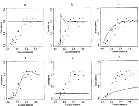
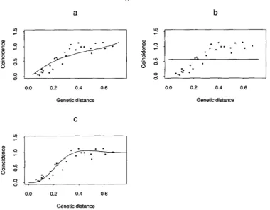
FIGURE 2.-Plots of coincidence us. genetic distance for the five-locus models. The points represent coincidence calculated from the data for each pair of atomic intervals among the nine loci. The corresponding genetic distance for each pair is calculated between the midpoints of the two intervals. The curves represent five-locus model coincidences. a is the Poisson model, b is the hard-core model, c the King-Mortimer model, d the gamma model, e the count-location model and f the K-M I1 model.

The results shown for the Poisson are from a calculation rather than from simulation, but the simulated results are virtually identical. In the case of the gamma model, the likelihood can actually be calculated in the case of integer-shape parameter (ZHAO et al. 1995a). In the nine-locus case using this likelihood calculation, the best fit is obtained using shape parameter 5 , which agrees with the results given here for the nine-locus case. This would correspond to four gene conversion events be- tween each crossover in the framework described in Foss et al. ( 1993). The count-location model has previously been fit to the MORGAN et al. ( 1935 ) dataset by RSCH

and LANCE ( 1983), using a calculated, rather than simu-

lated, likelihood. In their calculation they did not pool events in which three or more recombinations occurred. Thus, they maximized a slightly different likelihood than the one maximized here. Still, the results are very close to those obtained here. Note that the estimates of genetic distances and their standard deviations were fairly similar for all models. The Poisson model gives very similar esti-

mates to the other models for small genetic distances ( <10 cM) but overestimates larger genetic distances rel- ative to the other models.

The SDs were estimated by simply taking numerical derivatives of the recombination probabilities ( p i s in the notation given above) with respect to the estimated parameters and using these to calculate the Fisher infor- mation matrix. A better approach, not taken here, would be to smooth the likelihood surface before calcu- lating derivatives.

a

b C

0

’1

2

I

d

n

I

Poiss K-M I I Ct-loc Gamma

2J

,

Poiss K-M It Ct-loc Gamma

e

I Poiss K-M II Ct-loc Gamma

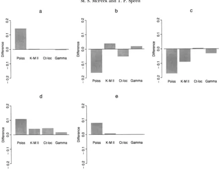
FIGURE 3.-Distribution of the number of crossovers among all nine loci of the MORGAN et al. ( 1935) dataset for each of the models under consideration relative to the data distribution. ( a ) The chance of zero crossovers for each of the models minus 0.056, the proportion of cases in which zero recombinations occurred in the data. (b-e) Similar bar graphs for the probabilities of 1, 2, 3 and 4 or more crossovers, respectively. The data proportions to which these numbers are compared are 0.485, 0.429, 0.030 and 0, respectively.

of the number of single recombination events among the five loci and an overestimate of all other types of recombination events. Figure 3 shows that in the nine- locus case, the Poisson model predicts too few single and double crossover events and too many of all other types. The gamma, count-location and K-M

I1

models all do well at matching the distribution of the number of crossovers in the data, although the K-M

I1

model does not do nearly as well with nine loci and with five. The other aspect of the models which we shall con- sider is the coincidence function which is discussed above. Figure 2 shows coincidence us. genetic distance for the five-locus models, and Figure 4 shows it for the nine-locus models. Recall that coincidence is a measure of the degree to which one crossover inhibits the forma- tion of another nearby. For the Poisson model coinci- dence is one, reflecting no interference. The coinci- dence curves for the models have been calculated (or simulated, in the case of the King-Mortimer and K-M

I1

models) using infinitesimal intervals. The coincidence curves of the gamma model and the King-Mortimer

model give the best approximation to the data in the five-locus case, whereas the gamma and

K-M

I1

models do best in the nine-locus case.

The strange shape of the coincidence curve for the hard-core model can be explained as follows: in the hard-core model, no points are allowed within a fixed distance of the crossover point that is assumed to lie at

Modeling Interference

a

b

1043

- /

..

..

e .

0.0 0.2 0.4 0.6 0.0 0.2 0.4 0.6

Genetic distance Genetic distance

C

0.0 0.2 0.4 0.6

Genetic distance

FIGURE 4.-Plots of coincidence us. genetic distance for the nine-locus models. The points represent coincidence calculated from the data for each pair of atomic intervals among the nine loci. The corresponding genetic distance for each pair is calculated between the midpoints of the two intervals. The curves represent nine-locus model coincidences. a is the K-M I1 model, b is the count-location model and c is the gamma model.

It should be noted that the coincidence curve for the count-location model is constant, even if the distribu- tion of points is i.i.d. but nonuniform. The reason is that the x axis represents genetic, not physical distance, that is, it represents the expected number of crossovers and so is automatically rescaled to be uniform. Note also the anomaly that the K-M I1 model fits the data better (according to chi-square) in the five-locus case than in the nine-locus case, but the coincidence curve resembles the data much more closely in the nine-locus case.

DISCUSSION

Although none of the models fit the data, several of the models were able to capture certain aspects of the data. The best overall model of the ones considered was the renewal model with gamma interarrivals. It gave reasonable estimates of the numbers of crossovers and matched the interference pattern in the data as mea- sured by the coincidence. In terms of the chi-square statistic, the gamma model represents a huge improve- ment over the Poisson model. Furthermore, in the case of integer shape parameter, the gamma model may prove tractable enough to use in mapping applications. This work represents a first attempt to systematically

fit a range of point process models to recombination data. A suitable model, such as the gamma model, may be of great use in assessing the impact of interference on conventional linkage analyses and genetic mapping. It may even be possible to apply such a model in genetic mapping, thereby making more efficient use of the data.

We are grateful to B. D. RIPLEY for his advice on the Monte Carlo method and to F. W. STAHI. for helpful discussions. This work was supported by National Science Foundation grants DMS880237 and DMS9113527.

LITERATURE CITED

CARTER, T. C . , and A. ROBERTSON, 1952 A mathematical treatment of genetical recombination using a four-strand model. Proc. R. SOC. Lond. Ser. B 139: 410-426.

COBBS, G., 1978 Renewal process approach to the theory of genetic linkage: case of no chromatid interference. Genetics 89: 563- 581.

COX, D. R., and V. ISHAM, 1980 Point Processps. Chapman and Hall, New York.

DIGGLE, P. J., and R. J. GRATTON, 1984 Monte Carlo methods of inference for implicit statistical models. J. Roy. Statist. SOC. B 46:

193-227.

EVANS, S. N., M. S. MCPEEKand T. P. SPEED, 1992 A characterisation of crossover models that possess map functions. Theor. Popul. Biol. 43: 80-90.

Foss, E., R. LANDE, F. W. STAHI. and C. M. STEINBERG, 1993 Chiasma interference as a function ofgenetic distance. Genetics 133: 681- 691.

GOLDGAR, D. E., and P. R. FAIN, 1988 Models of multilocus recombi- nation: nonrandomness in chiasma number and crossover posi- tions. Am. J. Hum. Genet. 43: 38-45.

HALDANE, J. B. S., 1919 The combination of linkage values, and the calculation of distances between the loci of linked factors. J. Genet. 8: 299-309.

JOHNSON, W. A,, and R. F. MEHI., 1939 Reaction kinetics in processes of nucleation and growth. Trans. A.I.M.M.E. 135: 416-458. K A R I J N , S . , and U. LIBEKMAN, 1979 A natural class of multilocus

recombination processes and related measures of crossover inter- ference. Adv. Appl. Probab. 11: 479-501.

LANDE, R., and F. W. STAHL, 1993 Chiasma interference and the distribution of exchanges in Drosophila melanogaster. Cold Spring Harbor Symp. Quant. Biol. 58: 543-552.

LIBERMAN, U., and S . KARLIN, 1984 Theoretical models of genetic map functions. Theor. Popul. Biol. 25: 331-346.

KING, J. S., and R. K. MORIIMER, 1990 A polymerization model of chiasma interference and corresponding computer simulation. Genetics 126 1127- 1138.

MEIJERING, J. L., 1953 Interface area, edge length, and number of vertices in crystal aggregates with random nucleation. Philips Res. Rep. 8: 270-290.

MORGAN, T. H., C . B. BKIDGES and J. SCHUI.TZ, 1935 Constitution of the germinal material in relation to heredity. Carnegie Instit. Washington Publ. 34: 284-291.

MORTIMEK, R. K., and S . FOGEI., 1974 Genetical interference and gene conversion, pp. 263-275 in Mechanisms in Recombination,

edited by R. F. GKEI.I.. Plenum, New York.

MIJI.I.EK, H. J,, 1916 The mechanism of crossing-over. Am. Nat. 50:

NELDER, J. A., and R. MFAD, 1965 A simplex method for function 193-221, 284-305, 350-366, 421-434.

minimisation. Comput. J. 7: 303-313.

OWEN, A. R. G., 1949 The theory of genetical recombination, 1.

Long-chromosome arms. Proc. R. Soc. Lond. Ser. B 136 67-94. OWEN, A. R. G., 1950 The theory of genetical recombination. Adv.

Genet. 3: 117-157.

PASCOE, L., and N. E. MORTON, 1987 The use of map functions in multipoint mapping. Am. J. Hum. Genet. 4 0 174-183. PAYNE, 1.. C., 1956 The theory of genetical recombination: a general

forrnulation for a certain class of intercept length distributions appropriate to the discussion of multiple linkage. Proc. R. Soc. Lond. Ser. B 1 4 4 528-544.

&PIXY, B. D. R., 1987 Stochastic Simulation. John Wiley and Sons, New York.

RISCH, N., and K. LANGF., 1979 An alternative model of recombina- tion and interference. Ann. Hum. Genet. 43: 61-70.

RISCH, N., and K. LXNGE, 1983 Statistical analysis of multilocus re- combination. Biometrics 39: 949-963.

SPEED, T. P., M. S. MCPEEK and S. N. EVANS, 1992 Robustness of the ntrinterference model for ordering genetic markers. Proc. Natl. Acad. Sci. USA 89: 3103-3106.

STAHI., F. W., 1979 h e t i c Recombination. Thinking About it in Phage and Fungi. W. H. Freeman, San Francisco.

STAM, P., I979 Inte~ference in genetic crossing over and chromo- some mapping. Genetics 92: 573-594.

STOY.W, D., W. S. KENDAI.~. and J. MFCKE, 1987 Stochastic G?omel?y

and 2t.s Applications, Wiley, New York.

STUKTEVAVT, A. H., 1915 The behavior of the chromosomes as stud- ied through linkage. %. Indukt. Abstammungs. Vererbungsl. 13:

WEINSTEIN, A., 1936 The theory of multiple-strand crossing over. Genetics 21: 155-199.

ZHAO, H., T. P. SPEEI) and M. S. MCPEEK, 1995a Statistical analysis of crossover interference using the chi-square model. Genetics

ZHAO, H., M. S. MCPEEK and T. P. SPEED, 1995b Statistical analysis 234-287.

139: 000-000.

of chromatid interference. Genetics 139: 000-000.