Risk Informed Validation Framework Using Bayesian Approach.

(1)

ABSTRACT

BODDA, SARAN SRIKANTH. Risk Informed Validation Framework Using Bayesian Approach. (Under the direction of Dr. Abhinav Gupta.)

(2)

(3)

Risk Informed Validation Framework Using Bayesian Approach

by

Saran Srikanth Bodda

A dissertation submitted to the Graduate Faculty of North Carolina State University

in partial fulfillment of the requirements for the Degree of

Doctor of Philosophy

Civil Engineering

Raleigh, North Carolina 2020

APPROVED BY:

Dr. Kumar Mahinthakumar Dr. Brian Reich

Dr. Kevin Han Dr. Abhinav Gupta

(4)

DEDICATION

(5)

BIOGRAPHY

Saran Srikanth Bodda was born and brought up in the city of Vizag in India. He joined the undergraduate program in Civil Engineering at Indian Institute of Technology, Guwahati, India in 2010 and received the Bachelors of Technology degree in July, 2014. He joined North Carolina State University in Spring 2015 to pursue his Master of Science in Civil Engineering. After his M.S., he continued to pursue his doctoral degree in Structural Engineering and Mechanics and minor in Statistics at North Carolina State University.

Saran is a member of two honor societies, Tau Beta Pi and Chi Epsilon at NC State University. He also interned at Idaho National Laboratory in the summer of 2017. He has received the Paul Zia graduate fellowship award for Structural Engineering from the department of CCEE at NC State University in 2019. The work presented in Part II of this dissertation got him recognized as one of the three winners of the Shibata Early Career Award at SMiRT 25 Conference, 2019.

(6)

ACKNOWLEDGEMENTS

Firstly, I would like to express my sincere gratitude to my advisor, Dr. Abhinav Gupta, for giving me the opportunity to pursue my graduate studies at NCSU. His patience, motivation, immense knowledge and constant guidance helped me during the entire research work and in writing this dissertation. I would also like to thank Dr. Nam Dinh, Dr. Kumar Mahinthakumar, Dr. Brian Reich, and Dr. Kevin Han for graciously agreeing to serve on my advisory committee and for their valuable suggestions.

I am always grateful to my undergrad advisor, Dr. Hrishikesh Sharma, for enlightening me with the first glance of research. I am extremely grateful to Dr. Shinyoung Kwag, Dr. Paridhi Athe, and Dr. Linyu Lin for their input and feedback without which this research could not have been possible. I am always thankful to Ankit Dubey, a valued friend, without whom it would be impossible to imagine PhD life. A very special thanks to Harleen and Pragya, for giving me happiness, strength and keeping me in high spirits when I felt troubled. I thank my colleagues and friends – Krishna, Uday, Akshay, Payel, Sugandha, Nick, Sangwoo, Parth, Alexis, Jimmy, Abraham, Revanth, Ankith, Arpit, STP, Sheik, Raj, and Abhinab for their precious support and for the wonderful time I spent with them during my stay in Raleigh.

(7)

(8)

LIST OF TABLES

Table II.1 CPTs of all the nodes in the Compact Bayesian network . . . 23

Table II.1 Continued . . . 24

Table II.2 Description of VUQ Quality grade for different Data Applicability attributes . . . 29

Table II.3 Quantification of Maturity level for Data Applicability . . . 29

Table II.4 Simulation and Data-driven fragility parameters . . . 41

Table II.5 Grade quality of Validating events . . . 42

Table II.6 Additional Failure data of DG Failure event . . . 46

Table III.1 Lognormal Fragility parameters of basic events . . . 61

Table III.2 Fussell-Vesely Importance measure for Building-Piping System Failure 61 Table III.3 Simulation and Data-driven fragility parameters (Case 1) . . . 65

Table III.4 Overlapping Coefficient of all the events (Case 1) . . . 65

Table III.5 Simulation and Data-driven fragility parameters (Case 2) . . . 69

Table III.6 Simulation and Data-driven fragility parameters (Case 3) . . . 70

Table III.7 Additional Failure data of events E1 and E2 . . . 71

Table III.8 Description of VUQ Quality grade for different Data Applicability attributes . . . 75

Table III.9 Maturity levels for Code Adequacy . . . 77

Table III.10 Percentage of Maturity Levels for Code Adequacy . . . 83

Table IV.1 Simulation-based lognormal fragility parameters of basic events (ˆλ = Median, βAU = Lognormal standard deviation) . . . 108

(11)

(12)

LIST OF FIGURES

Figure II.1 Flowchart of proposed model validation method (Kwag et al. [13]) 16

Figure II.2 Overlapping Coefficient . . . 18

Figure II.3 Generic Event tree . . . 21

Figure II.4 Compact Bayesian Network representation of Generic Event tree . 22 Figure II.5 Bayesian Network representation of Generic Event tree . . . 23

Figure II.6 Family of Data-driven fragility curves corresponding to different maturity levels of Data Applicability (IM – Intensity Measure) . . 30

Figure II.7 Flowchart of Proposed Framework with Data Applicability . . . 32

Figure II.8 Accident sequence layout of Synthetic Example . . . 35

Figure II.9 Event Tree logic for the synthetic example . . . 35

Figure II.10 Weighted Mean Storm Surge Hazard Curve . . . 36

Figure II.11 Fault Tree of Protective Floodwall event . . . 37

Figure II.12 Loss of Onsite AC Power Scenario . . . 40

Figure II.13 Variation of Discharge Coefficient, Cd . . . 40

Figure II.14 Simulation and Data-driven (median) fragility curves . . . 43

Figure II.15 Histogram of TOP events Overlapping Coefficients . . . 45

Figure II.16 OC Histogram of DG Failure and End state (System-level) . . . 46

Figure III.1 Flowchart of risk informed validation framework [14] . . . 54

Figure III.2 Fault tree for Building-Piping System Failure . . . 60

Figure III.3 Bayesian Network for Building-Piping System Failure . . . 60

Figure III.4 Consistency Index, δ= 1 . . . 63

(13)

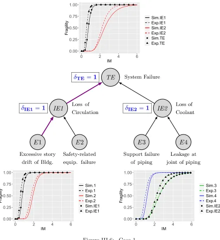
Figure III.6 Case 1 . . . 66

Figure III.7 Consistency Index for Loss of Coolant Event (δIE2 = 0, Case 2) . . 67

Figure III.10 Case 3 Updated . . . 73

Figure III.11 Bayesian network for Code Adequacy . . . 74

Figure III.12 Diesel generator failure . . . 78

Figure III.13 Simulation and Data-driven (median) fragility curves . . . 79

Figure III.14 Overlapping Coefficient vs J-Divergence . . . 80

Figure III.15 Simulation-based fragility curves with epistemic uncertainty . . . . 81

Figure III.16 Data-driven fragility curves with high (left) and very low (right) maturity of Data Applicability . . . 81

Figure III.17 Histogram of DG failure event Overlapping Coefficients with high (left) and very low (right) maturity of Data Applicability . . . 82

Figure IV.1 EMDAP Framework [10] . . . 91

Figure IV.2 Integrated Risk informed EMDAP framework . . . 94

Figure IV.3 Plant Layout [43] . . . 96

Figure IV.4 Event Tree logic for the Sunny Day Dam failure . . . 97

Figure IV.5 Fault Tree of Event 1: EF-PROTECT . . . 98

Figure IV.6 Fault Tree of Event 3: EF-ERLYPOW . . . 99

Figure IV.7 Fault Tree of Event 4: EF-RCNTRL . . . 100

Figure IV.8 Fault Tree of Event 5: EF-NOLOCA . . . 102

Figure IV.9 Fault Tree of Event 6: EF-RPRESS . . . 103

(14)

Figure IV.11 Fault Tree of Event 9: EF-MSSVS . . . 105 Figure IV.12 Event Tree for Case 1 . . . 110 Figure IV.13 Simulation (median) fragility curves for TOP events (Case 1) . . . 111 Figure IV.14 Code Adequacy of system-level event (Case 1) . . . 111 Figure IV.15 Simulation and Data-driven fragility curves of critical event (Case 1) 112 Figure IV.16 Event Tree for Case 2 . . . 113 Figure IV.17 Simulation fragility curves for system-level and critical events (Case

(15)

PART I

(16)

I.1 Introduction

In recent years, safety of nuclear facilities against external hazards has gained significant importance. Fukushima Daiichi nuclear disaster occurred due to tsunami induced flooding [1]. In United States, the South Texas Project nuclear plant was shut down when floods due to hurricane Harvey threatened the nuclear plant [2]. Several nuclear power plants (Oyster Creek, Indian Point, Nine Mile Point, and Salem) in the US were shut down due to flooding from hurricane Sandy [3]. Subsequently, the nuclear industry has led the development of risk-informed design and decision making approaches for the safety assessment of nuclear power plants against external flooding hazard. This requires appropriate characterization of uncertainties in the understanding of physical phenomenon and in the advanced simulation models that are used to represent them. This research develops a robust risk informed framework for validation of advanced simulation codes with a probabilistic criterion for adequate level of validation.

I.2 Background

Probabilistic risk assessment for external flooding hazard typically involves three technical elements: (i) probabilistic flood hazard assessment (PFHA), (ii) performance based flooding fragility curves, and (iii) fault tree/event tree model of the plant response to an external flooding event [4]. The reliability of fragility curves that are generated by high-fidelity simulation codes is assessed primarily by validation process.

The formal definition of Verification and Validation (V&V) is [5, 6, 7]:

(17)

represents the underlying mathematical model and its solution.”

• Validation – “The process of determining the degree to which a model is an accurate representation of the real world from the perspective of the intended uses of the model.”

Loosely speaking, verification deals with the problem “are we solving the equations right”? and validation deals with “are we solving the right equations”? [8].

A validation framework should be able to capture all sources of uncertainty due to incomplete knowledge and inherent randomness in the performance of the system as well as in the characterization of the external hazard. The range of applicability of a computational tool is assessed by the physics and the models it contains. Verification, Validation, and Uncertainty Quantification (VVUQ) methodology helps to assess the adequacy of simulation codes in predicting the credibility of risk assessments and the uncertainty associated with those predictions.

Fields such as computational fluid dynamics and heat transfer, computational solid mechanics, and computational integrated system thermal fluids behavior have developed their own set of guidelines for V&V in modeling and simulation. The widely used frameworks for VVUQ in nuclear power plant safety applications are:

(1) Code Scaling, Applicability, and Uncertainty methodology (CSAU)

(18)

• Requirements and Code Capabilities – It includes various components such as identification of the accident scenario and nuclear power plant to be analyzed, establishment of phenomena resolution using PIRT process, and specification of frozen simulation code with complete documentation.

• Assessment and Ranging of Parameters – This element focuses on validation by establishment of an experimental database which consists of relevant separate effect tests (SETs) and integral effect tests (IETs). An assessment matrix is created based on SETs and IETs for all the phenomena identified in element 1. Scaling effects of the code are determined by performing simulations of different reduced scale test facilities. Bias and uncertainty are estimated for all the evaluated quantities.

• Sensitivity and Uncertainty Analysis – The final element performs sensitivity analysis and UQ by combining the biases and uncertainties due to all the sources. Response surface method is used to evaluate the effect of uncertainty from the range of input parameters.

(2) Evaluation Model Development and Assessment Process (EMDAP)

In 2005, USNRC Regulatory Guide 1.203 introduced EMDAP which is a systematic process to confirm the adequacy of a particular code to analyze transient and accident behavior that is within the design basis of a nuclear power plant. The key steps involved in the EMDAP process are listed below [10]:

• Identification of analysis purpose, figures of merit (FOM), mathematical modeling methods, components, phenomena, and physical processes.

• Hierarchical breakdown of systems, phenomena and process.

(19)

• Development of evaluation model (EM) with state-of-the-art modeling tools and algorithms.

• Assessment of EM models adequacy using a two-tier review process (top-down and bottom-up). The bottom-up approach focuses on the fundamental building blocks of the code in which closure and correlation models are evaluated by considering their fidelity to fundamental or SET data, and scalability. The top-down approach focuses on capabilities and performance of the EM in which field equations and numeric solutions are evaluated by considering their fidelity to component or IET data, and scalability.

• Characterization of EM bases and uncertainties.

(3) Predictive Capability Maturity Model (PCMM)

Sandia National Laboratories (SNL) developed PCMM to assess the maturity of modeling and simulation tools for nuclear weapon applications. However, the elements of PCMM can be applied to broad range of engineering applications. PCMM is a model which assesses the confidence one should place in computational tools by evaluating the maturity level of the following six fundamental attributes [11]:

• Representation and geometric fidelity – level of detail specified in physical modeling of the system (spatial and temporal). Ranging from simple model relying on expert judgment to CAD modeling of the real system.

• Physics and material model fidelity – the degree that models are physics based and how much they are calibrated. Models typically range from fully empirical to complete physics based.

(20)

no formal verification testing to rigorous benchmark solutions testing.

• Solution Verification – assessment of numerical solution errors and confidence in the computational results. Ranging from no formal assessment to error estimation of all system response quantities (SRQs) by performing quantitative error estimation methods.

• Model Validation – assessment of physical accuracy of the computational model by comparing with experimental measurements, and relevancy of the experimental conditions. Ranging from no comparison with experimental data to comparison of computational results with an extensive database of both SET and IET experiments.

• Uncertainty quantification and sensitivity analysis – identification of sources of uncertainty, the effect of uncertainty on computational results, and the determining the critical parameters that contribute to uncertainty in system responses. For high maturity levels, aleatory and epistemic uncertainties are comprehensively treated.

(4) Predictive Capability Maturity Quantification (PCMQ)

CSAU, EMDAP, and PCMM are all expert elicitation methodologies and these frameworks does not give any guidance on quantification methods for making decision on reliability of a simulation tool. PCMQ framework addresses this issue by formalizing the validation process as structured knowledge representation, information abstraction, multilevel evidence incorporation, which is further quantified as a decision-making process for nuclear reactor engineering or safety application [12].

(5) PRA based model validation method using Bayesian network

(21)

the context of external hazard PRA. This methodology employs a probabilistic index to quantify the degree of validation within the context of uncertainty. In this approach, logic trees for system level performance are mapped into a Bayesian Network (BN) that allows formal propagation of uncertainty at component-level validation to assess the degree of validation at system-level. It uses Bayesian inference for identifying the risk-consistent events along a critical path and evaluates the need for additional validation that may be required. Identification of critical path from a validation standpoint within a risk-informed framework in this approach provides a basis for improving the overall validation through identification of specific events along the critical path. The overall validation can be improved either by enhancing the simulation models of components along the critical path or by collecting additional validation data until the adequacy of the system level validation is satisfied. Application of the framework proposed by Kwag et al. [13] was illustrated for two case studies related to the performance of structure, system, or component (SSCs) subjected to earthquake hazard.

I.3 Research Objectives

The primary objective of this research is to develop a framework for system-level validation based on a risk consistent approach against external flooding hazard. The key objectives of the proposed research are outlined as follows:

• Formally include the quality of experimental data in a quantitative assessment through validation uncertainty quantification (VUQ).

(22)

• Identify the critical events which are consistent with both simulation and data-driven models.

• Assess the maturity of the adequacy of a simulation tool for an intended application.

• Update the evaluation (simulation or data-driven) models to obtain a desirable acceptance criterion using Bayesian inference.

• Integrate risk informed validation methodology into EMDAP framework for a wider applicability of the framework.

• Illustrate the effectiveness of the proposed framework to a synthetic example and a realistic example based on NRC working example.

I.4 Proposed Research

The following tasks are needed to accomplish the objectives mentioned in this research:

I.4.1 Risk Informed Validation Framework for External Flooding Scenario

In this research, we illustrate the application of performance based risk-informed validation framework proposed by Kwag et al. [13] to an external flooding event. However, it is determined that a direct application of this approach to flooding is restricted due to a lack of relevant data to evaluate experimental fragilities for flooding failures. Therefore, we take a simple synthetic example to evaluate the applicability of the proposed framework to validation of flooding PRA scenario and update the proposed framework as needed. The specific tasks undertaken to conduct this research are:

(23)

probability of top events in the event tree.

• Develop an assessment base which consists of experimental data at component level and subsystem level. Grade the quality of available experimental data and introduce the concept of data-driven fragility.

• Develop performance-based simulation and data-driven fragility curves.

• Develop a mapping algorithm for the transformation of an Event tree into a Bayesian network. Map the event tree and the corresponding fault trees into the Bayesian network.

• Propagate fragilities from basic events to intermediate-level events and ultimately to system-level event through the Bayesian network.

• Identify the critical events based on simulation models or data-driven models.

• Use Overlapping coefficient (OC) as the validation index to quantify the degree of validation within the context of uncertainty.

• CalculateOCsin component-level using simulation and data-driven fragility curves.

• Evaluate system-level OC and improve it by enhancing the simulation model or collecting additional experimental/field data for the critical events if required.

I.4.2 Enhancement of Existing Risk Informed Validation Framework

(24)

for a complete and wider applicability of the framework. The specific tasks required to achieve the objectives of this research is summarized below:

• Identify the critical path that leads to system-level failure by using the concept of importance measures.

• Introduce the concept of Consistency Index which ensures that the simulation and data-driven fragilities correspond to the same set of critical events.

• Incorporate and interpret the consistency index in the risk informed validation framework through various case studies.

• Assess the decision regarding the adequacy of a simulation code for an intended application using the concept of maturity level.

• Develop an additional attribute Code Adequacy (CA) in terms of Validation Result (VR) and Data Applicability (DA) attributes for validation assessment.

• Label maturity levels as very low, low, medium, and high (increasing order of value).

• Compare the validation results for two types of validation metric: Overlapping coefficient and Kullback-Leibler divergence.

• Illustrate the effectiveness of the enhanced methodology for a simple example of flooding risk assessment.

I.4.3 Assessment of Risk Informed Validation Framework to a Real Life Like

Application – Sunny Day Dam Failure

(25)

integration of the proposed risk informed methodology into Evaluation Model Development and Assessment Process (EMDAP) framework. The specific tasks undertaken to conduct this research are:

• Integrate risk informed validation methodology into EMDAP framework.

• Develop event tree and the corresponding fault trees for the realistic flooding scenario of the Sunny Day Dam failure.

• Identify non-physical events that are not sensitive to hydrodynamic and fragility modeling.

• Handle the non-physical events by treating them as either completely safe or fail.

• Illustrate the integrated framework to the realistic flooding scenario.

I.5 Organization

(26)

PART II

Risk Informed Validation Framework for

(27)

II.1 Introduction

In recent years, flooding at nuclear power plants (NPP) has increased emphasis on considering advanced simulation codes to evaluate the vulnerability of nuclear plants. Absence of a complete and sufficient verification and validation (V&V) of advanced simulation codes results in adoption of greater uncertainty by experts in risk informed evaluations which in turn leads to conservative assumptions. Past experience has shown that such conservative assumptions in the context of safety assessment for other external hazards such as seismic have resulted in highly over-designed nuclear power plant systems and excessively high costs. Therefore, it is quite important that various uncertainties in this process are appropriately identified and included through formal uncertainty quantification (UQ). A robust framework for verification and validation is needed to not only include uncertainties but also to formalize the confidence in predictions of PRA studies that are based on advanced simulations.

(28)

In this manuscript, a synthetic flooding scenario is used as case study to allow a preliminary interrogation of the proposed framework. It is determined that a direct application of Kwag et al. [13] approach to flooding is restricted due to a lack of relevant data to evaluate experimental fragilities for flooding failures. As experimental data is scarce and expensive, modification to the existing framework is needed in order to utilize the data from existing, somewhat related, and diverse experimental studies for validation of certain aspects. To be more precise, a modification is needed to formally include the quality of experimental data in a quantitative assessment through what is often termed as validation uncertainty quantification (VUQ). Furthermore, the available experimental data is not directly related to the failure of SSCs for flooding conditions. Instead, the data typically relates to the various parameters of a hydrodynamic and fluid flow simulations which is related to fragility assessment only indirectly. In fact, one may use a historically well-established empirical model based on many years of research and laboratory studies to determine fluid flow conditions. Consequently, it is proposed to replace “experimental fragility” in the existing framework by “data-driven fragility.”

(29)

errors. The proposed modification grades the R/S/U attributes based on their VUQ quality and incorporates each of them quantitatively in the data-driven fragility analysis.

Existing framework proposed by Kwag et al. [13] uses a mean fragility curve that results in a point estimate for the validation index. However, fragility assessment of a flooding related event suffers from large epistemic uncertainty making a point estimate for validation index less meaningful. Therefore, we propose a modification to the existing framework which considers multiple fragility curves using different confidence levels instead of just the mean fragility curve. Based on these multiple curves, the validation metric changes from a point estimate to a distribution.

(30)

II.2 Summary of Risk Informed Validation Framework by Kwag et al. [13]

The existing framework of Kwag et al. [13] employs two key stages that are described below. The complete framework is illustrated through the flowchart in Figure II.1.

Construct Fault Tree (FT) for system risk analysis. Map FT into Bayesian Network. Evaluate system risk and identify

the most critical scenario. Pick out important components

in identified critical path. Introduce overlapping coefficient

(OC) as a validation metric. Calculate OCs in component level using simulation & experimental data.

Is mechanistic model to relate nodes available? Determine

response surface.

Evaluate fragilities for Intermediate event and Top event by simulation and

experimental fragilties of components. Use fragility data to calculate OC.

If new data is available in any levels, update OCs of all levels based on the data.

Decision (System OC>Criterion)

System level validation process is done.

Improve simulation model of components in

identified critical path.

STAGE 1 STAGE 2 YES NO YES NO

(31)

Stage 1:

The initial step involves development of a fault tree for the given scenario. The risk of basic events is calculated by convoluting the hazard curve under consideration with the corresponding fragility curve using Eq. (II.1).

Pf =

Z

Pf|λ(λ)

dH(λ)

dλ

dλ (II.1)

where, λ is the hazard intensity measure. H(λ) is the hazard curve, representing annual exceedance frequency for λ. Pf|λ is the fragility curve which represents the conditional probability of failure givenλ.

The fault tree is mapped into a Bayesian network in order to account for non-binary and statistical relationships between events. Then, a system analysis is carried out to identify the important events along the critical path with respect to the overall system-level risk. The entire framework is based on the definition of an overlapping coefficient that is used as the validation index to quantify the degree of validation within the context of uncertainty.

Definition of Overlapping Coefficient

Overlapping coefficient (OC) is simply defined as the percentage of overlapping area between two probability density curves (Figure II.2) and is given by Eq. (II.2). OC

(32)

OC = Z

Rn

min(f₁(x), f₂(x))dx (II.2)

Simulation Data

Experimental Data

Figure II.2: Overlapping Coefficient

Stage 2:

In Stage 2, Overlapping coefficients are calculated for all the basic events based on the corresponding simulation and experimental (or data-driven) fragility curves. The fragility curves are propagated from basic events to intermediate-level events and ultimately to system-level events through the BN using either mechanistic relationships or response surfaces between the component-level and upper-level nodes. Then, the overlapping coefficients are evaluated for all the nodes using the fragility information. At this stage, if new information becomes available then the OCs are updated.

(33)

validation can be improved either by enhancing the simulation models of components along the critical path or by collecting additional validation data until the adequacy of the system level validation is satisfied.

II.3 Consideration of Event Trees in the Proposed Framework

The framework by Kwag et al. [13] was based on using Fault trees for risk assessment and it did not consider Event tree for representing the event failure against a seismic hazard. In general, a complete risk assessment requires a combination of fault trees and event tree that are connected together. Specifically, in a flooding scenario it is important to evaluate the sequence of events through an event tree and each top event in the event tree can have its own fault tree. Therefore, in this manuscript we extend the existing framework to include both the event tree and the corresponding fault trees.

(34)

II.3.1 Event tree analysis

Event trees are widely used to analyze accident scenarios in PRA. Event tree analysis uses a (Boolean) logical modeling technique that shows all possible outcomes arising from a single accident event by taking into account multiple safeguards or barriers which are placed as protective features to deal with the accidental event. While the methodology presented in this manuscript is quite generic and can incorporate dynamic nature of events, only static event trees are considered for simplicity of illustrating the methodology.

An Event tree starts with an initiating (accident) event, such as an external/internal hazard. The failure or success consequences (outcomes) of the initiating event are followed through a series of possible branches or paths. The frequencies of various possible outcomes are calculated by assigning a conditional probability of occurrence for each branch and a frequency for the initiating event. Figure II.3 shows a generic example of how an event tree can be drawn. The green lines show the success paths and the red lines show the failure paths. Usually, the failure probabilities (Pf) of intermediate events are calculated from a fault tree analysis and the success probabilities (Ps) of the events are calculated as: Ps = 1−Pf. The overall (end state) frequency of occurrence of a path is calculated by multiplication rule i.e. multiplying all the conditional probabilities of events in that specific path with the frequency of the initiating event. The end state frequency of path A as shown in Figure II.3 is given by Eq. (II.3).

FA=P (IE.1s.2s.3s.4s1)

=F (IE)P(1s_|IE)P (2s_|1s.IE)P (3s_|2s.1s.IE)P(4s1|3s.2s.1s.IE)

(35)

Initiating Event (IE)

Success (1s)

Success (2s)

Success (3s)

Success (4s1) FA=FIEP1sP2sP3sP4s1

Failure (4f1) FB=FIEP1sP2sP3sP4f1

Failure (3f)

Success (4s2) FC=FIEP1sP2sP3fP4s2

Failure (4f2) FD=FIEP1sP2sP3fP4f2

Failure (2f) FE=FIEP1sP2f

Failure (1f) FF=FIEP1f

Initiating Event Event 1 Event 2 Event 3 Event 4 Outcome

Figure II.3: Generic Event tree

II.3.2 Mapping Algorithm

Accident sequences are first created using an Event tree (ET) due to its simplistic representation. The transformation of an event tree into a Bayesian network (BN) is done in three steps [16]:

1. convert branching points or events in ET into nodes in BN.

2. convert branches or paths in ET into corresponding directional arcs between nodes in BN.

3. convert conditional probabilities in ET into conditional probability tables (CPT) in BN.

(36)

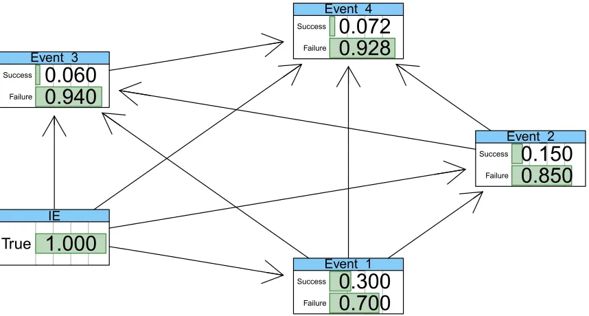
the compact BN are shown in Table II.1. When mapping an Event tree into a Bayesian network, the initiating event is represented as either occurred (True) or not occurred (False) rather than frequency due to conditional probability representation of nodes in a BN. Therefore, the outcome of all the end states is represented by probability. The frequency of end states can be obtained by simply multiplying the probability with the frequency of the initiating event. CPT of Event 2 has a third state E11f in addition to the states E21s and E21f, which is due to the branch coming out of Event 1 failure state. Node Event 4 is the last event in the BN, and it contains all the outcomes. An outcome node can also be created with total sum of failure (True) and success (False) state probabilities as shown in Figure II.4.

(37)

Figure II.5: Bayesian Network representation of Generic Event tree

Table II.1: CPTs of all the nodes in the Compact Bayesian network

(a) CPT of IE

States

T (True) PIE

F (False) 1₋PIE

(b) CPT of Event 1

States IE =T IE =F

E11s P1s 0

E11f P1f 1

(c) CPT of Event 2

States E1 = E11s E1 =E11f

E21s P2s 0

E21f P2f 0

(38)

Table II.1: Continued

(d) CPT of Event 3

States E2 =E2₁s E2 =E21f E2 =E11f

E31s P3s 0 0

E31f P3f 0 0

E21f 0 1 0

E11f 0 0 1

(e) CPT of Event 4

States E3 =E31s E3 =E31f E3 =E21f E3 =E11f

E41s P4s1 0 0 0

E4₁f P4f1 0 0 0

E42s 0 P4s2 0 0

E42f 0 P4f2 0 0

E21f 0 0 1 0

(39)

II.4 Data Applicability in Data-Driven Fragility

II.4.1 Fragility

Fragility curves are essential for assessing the vulnerability of an event, and offer a means of communicating the probability of damage over a range of potential hazard intensity measure levels. A fragility assessment requires characterization of failure in terms of a performance function, Z. The performance function defines the governing limit-state to evaluate the probabilities of failure. Fragility of systems, structures, and components (SSCs) is defined as the conditional probability of failure, Pf|λ , to exceed the defined performance function at a given measure of intensity parameterλ. Some of the commonly used Intensity measures (IM) are Flood height, Surge height, Peak ground acceleration (PGA), etc.

Z =Capacity₋Demand

Pf|λ(Z) = P(Z <0|λ)

(II.4)

Fragility analysis should account for all possible uncertainties in the SSCs. In the nuclear safety community, these uncertainties are broadly divided into two types [17, 18]:

1. Aleatory uncertainty – inherent randomness in the system’s performance as well as in the characterization of external hazard. This uncertainty is often irreducible and refer to as variability. Some of the sources of aleatory uncertainty are model parameters having random variability such as geometric dimensions, initial conditions, boundary conditions, or excitation load.

(40)

In practice, it might become blurry to distinguish between randomness and uncertainty.

The most common form of a fragility function is the log-normal cumulative distribution function (CDF) [19, 20].

λ= ˆλεEUεAU

Pf(Z|λ=λ∗) = Φ 



lnλ∗/ˆλ+βEUΦ−1(Q)

βAU





Pf,mean(Z|λ=λ∗) = Φ 



lnλ∗/ˆλ βmean





(II.5)

where,λ∗ corresponds to a particular value of the hazard intensity measure, λ. ˆλ

is the median capacity of resistance of SSCs against the hazard. εEU and εAU are variables representing epistemic and aleatory uncertainties about the median value. These variables are usually taken to be lognormal with unit median and logarithmic standard deviations of βEU and βAU, respectively. Q represents the confidence level in the estimated median capacity, ˆλ. βmean =

p

βEU2+βAU2 represents the combined uncertainty. Φ is the standard Gaussian cumulative distribution.

II.4.2 Data Applicability

(41)

used in Validation Uncertainty Quantification (VUQ). In this study, we incorporate a data-driven approach proposed by Athe [12] to quantify the quality of data used for generating data-driven fragility curves in terms of three attributes:

a. Relevance (R): Relevance reflects the degree of applicability of experimental data from an existing database to the current application “based on the preconceived view of phenomenology/process.”

b. Scaling (S): In many cases, the validation data for a flooding analysis is taken from scaled laboratory experiments. Therefore, when the same data is used for different larger scale applications, geometric scaling uncertainty should be incorporated to assess the similarity between reduced scale experiment and the full-scale application. Similarly, physics scaling uncertainty captures the degree of phenomena similarity between the applications. E.g. range of Reynolds number used in the prototype and full-scale application.

c. Data Uncertainty (U): Data uncertainty refers to the uncertainty (epistemic) in the measured data which arises due to sources such as instrument errors – accuracy and precision (resolution) of measuring instruments, data acquisition, and data processing.

(42)

analysis for different grade levels is quantified based on the following procedure.

1. For the data-driven fragility, with the perfect knowledge, the probability of failure is 0.5 at the median capacity. When epistemic uncertainty βEU is included, the fragility at median capacity becomes an uncertain variable.

2. If the grade level is high, then there is more confidence in the data. Therefore, there is very less uncertainty in the available experimental data for the intended application. This is quantified by varying the median fragility (= 0.5) with a uniform width of 0.1 ranging from -0.05 to 0.05.

βhigh = 0.5 +runif(−0.05,0.05) (II.6)

where, runif(a, b) generates a uniform random number from the interval (a, b) 3. Similarly, the epistemic uncertainty corresponding to a different grade level is

quantified using step (2) and Table II.3.

4. Then, the combined uncertainty of R/S/U is characterized by their weighted average:

βEU =wRβR+wSβS+wUβU (II.7)

In this study, the weights are considered to be equal for all the three attributes. 5. The new median capacity, ˆλ∗ is calculated by incorporating the epistemic

uncertainty due to R/S/U using the following expression:

ˆ

λ∗ = ˆλ/exp(qnorm(βEU)×βAU) (II.8)

(43)

6. Figure II.6 shows the uncertainty variation in data-driven fragility curves for different grade levels.

Table II.2: Description of VUQ Quality grade for different Data Applicability attributes

Attributes VUQ Quality – Grade

4 3 2 1

Relevance [R] Very High

(direct) High Medium Low

Scaling [S] Prototypic

(full-scale)

Adequately

scaled Medium

Inadequately scaled

Uncertainty [U]

Well-Characterized Characterized Medium

Poorly-Characterized

Table II.3: Quantification of Maturity level for Data Applicability

Grade Range of Uncertainty, β

(44)

1

0.7

0.4

0.1

(45)

II.5 Modified Risk Informed Validation Framework

As mentioned earlier in this manuscript, a modified framework is needed to enhance the originally proposed framework by Kwag et al. [13] due to three specific reasons:

1. For a systems level analysis, an event tree is necessary to represent the failure sequence of events resulting from an initiating flooding hazard. The framework is extended to include both the event trees and the corresponding fault trees for the representation of all possible accident scenarios and system-level performance. 2. When data from existing and related studies is utilized to evaluate experimental

fragilities for flooding failures, a formal approach is needed to include quality of experimental data. The framework is modified to incorporate the quality of experimental data quantitatively by adopting a data-driven approach.

3. In general, fragility assessment of a flooding related event suffers from large epistemic uncertainty. Therefore, for credibility of overall validation, probabilistic distribution of validation metric (overlapping coefficient) is required rather than a point estimate.

(46)

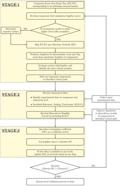
Construct Event Tree/Fault Tree (ET/FT) corresponding to an initiating external hazard

Develop component level simulation fragility curves

Is mechanistic model to relate higher level nodes available? Determine

response surface

Map ET/FT into Bayesian Network (BN)

Evaluate fragilities for Intermediate event and Top event from simulation fragilties of components

Evaluate system risk/fragility and identify the most critical scenario Pick out important components

in identified critical path

Develop Assessment Base

• Identify experimental data at component and subsystem level

• Establish Relevance, Scaling, Uncertainty (R/S/U) Develop Data-driven Fragility

Curves by including R/S/U

Introduce overlapping coefficient (OC) as a validation metric

Use fragility data to calculate OC

If new data is available in any levels, update OCs of all levels based on the data

Decision (System OC>Criterion?)

System level validation process is done

Improve simulation or data-driven models

of components in identified critical path

(47)

STAGE 1

• Develop an event tree to represent all possible accident scenarios resulting from an initiating external flood hazard.

• Construct required fault trees to obtain the failure probability of top events in the event tree.

• Develop simulation fragility curves for all the basic events. In general, fragility assessment requires use of a Monte Carlo approach to include uncertainties from various sources. However, if sufficient knowledge base has been developed then one can make use of the standard lognormal fragility parameters.

• Develop response surfaces between the basic events and intermediate events especially if a mechanistic relationship is not directly known.

• Map the event tree and fault trees into a Bayesian network.

• Evaluate system fragility by propagating the simulation fragility information from basic events through the Bayesian network.

• Identify critical events with respect to system vulnerability.

STAGE 2

• Develop an assessment base which consists of experimental data at component level and subsystem level.

• Establish Relevance, Scaling, and Data uncertainty (R/S/U) for the available experimental data using expert judgment.

• Generate data-driven fragility curves by including R/S/U as described in subsection II.4.2 Data Applicability.

(48)

fragility information.

STAGE 3

• Calculate overlapping coefficient based on simulation and data-driven fragility curves.

• At this stage if new data becomes available, update overlapping coefficients.

DECISION

• Compare system level overlapping coefficient with a predefined acceptance criterion.

• If the adequacy of system level validation is not satisfied collect more experimental data or improve simulation models of the identified critical events.

II.6 Illustration of Flooding Case Study

(49)

Floodwall

Landscape

Overflow Vent Overflow

DG Room

DG

Figure II.8: Accident sequence layout of Synthetic Example

II.6.1 Event Tree / Fault Tree Logic

The event tree resulting from this synthetic example is shown in Figure II.9, and includes the following top events:

Initiating Event (IE)

Success (1s) Safe

Failure (1f)

Success (2s) Safe

Failure (2f)

Success (3s) Safe

Failure (3f)

Success (4s) Safe

Failure (4f) Fail

Initiating Event Protective Floodwall

Plant Landscape

Protective Vent

Onsite

AC Power Outcome

Figure II.9: Event Tree logic for the synthetic example

IE – Initiating Event

(50)

weighted mean probabilistic storm hazard information from Dababneh and Weglian [24] shown in Figure II.10 for the risk calculation. In practice, the PFHA model should be developed for the site of interest.

0.2 0.4 0.6

100 10−1 10−2 10−3 10−4 10−5 10−6

Annual Exceedance Probability

Stor

m Surge Height [m]

Figure II.10: Weighted Mean Storm Surge Hazard Curve

Protective Floodwall

(51)

Protective Floodwall is Lost

External Flooding Elevation Overtops Floodwall

External Flooding Breach of Non-Overtopped Floodwall

NOT of Flood-Wall Overtopping

External Flooding Elevation Overtops Floodwall

Failure of Floodwall (from Fragility)

OR

AND

NOR

Figure II.11: Fault Tree of Protective Floodwall event

Plant Landscape

Plant landscape is used to describe the next top event in the event tree. This event is effective in preventing the flooding inundation (hlandscape) to exceed the height of

the vent (Hvent). The performance function for plant landscape failure is characterized

by following limit state:

Z_landscape =H_vent₋h_landscape (II.9)

And the conditional probability of landscape failure given storm surge height is expressed as:

Pf(Landscape|surge height) =P(ZLandscape <0) (II.10)

Protective Vent

(52)

out for these loads individually and later combined to obtain the failure probability of vent using a fault tree.

Onsite AC Power

The last top event in the synthetic example is the onsite AC power. This event is necessary to be maintained until hot shutdown is achieved. For this event, the performance function characterizes failure as DG failure. Failure occurs when water level in the DG room, h(t), due to vent overflow exceeds the height of the DG (HDG).

The performance function for DG failure is characterized by following limit state:

ZDG=HDG−h(t) (II.11)

And the conditional probability of DG failure given storm surge height is expressed as:

Pf(DG|surge height) =P(ZDG<0) (II.12)

The formulation for calculating water level in the DG room, h(t) is given by:

dh(t)

dt =

CdQ(t)_theoretical

A

Q(t)_theoretical=AventV =W p

2g∆H

(53)

Cd= Discharge Coefficient W = total height of vent opening

Q(t) = Discharge Rate g = acc. due to gravity

A_vent= Cross-Sectional Area ∆H = water height above the vent opening

V = Velocity

The discharge coefficient, Cd can exhibit uncertainty leading to change of water level in the DG room. The coefficient Cd can be calculated from experimental measured data (Reader-Harris and McNaught [26]) which is given by an empirical relationship, see Eq. (II.14), as well as formulated using a simulation model, see Eq. (II.15) [27]. The variation of Cd (probability density curves) for the experimental and simulation-based data is shown in Figure II.13. Now, we can estimate the water levels hvent, sim and

h_{vent, exp} in the DG room based on the simulation model ofCdand the experimental data of Cd. The simulation and data-driven (median) fragility curves for the DG failure can be generated based on hvent, sim and hvent, exp models, respectively.

Cd,exp = 0.5961 + 0.0261β2−0.216β8 + 0.000521

106β

ReD

0.7

+ "

0.0188 + 0.0063

19000β

ReD

0.8#

β3.5

106

ReD

0.3

+ (0.043 + 0.08e−10L1 ₋₀_.₁₂₃_e−7L1₎

×

"

1₋0.11

19000β

ReD

0.8#

β4

1₋β4 −0.031 "

2L0₂₋0.8

L0₂

1₋β

1.1#

β1.3

(II.14)

(54)

Figure II.12: Loss of Onsite AC Power Scenario

0.600 0.604 0.608

0

500

1500

density.default(x = C)

Discharge Coefficient

Density

Exp Sim

Figure II.13: Variation of Discharge Coefficient, Cd

II.6.2 Fragility Estimates and Data Applicability

(55)

inundation depends on the height of the water over the floodwall which in turn depends on the surge height. In order to have same intensity measure for all the events, it requires interaction between different models, software, and domains.

In this study, we assume that the simulation and the data-driven fragility information for all the top events is directly available. Table II.4 gives the lognormal fragility parameters for all the events. In practice, the fragility parameters are developed based on actual analysis of the site specific plant SSCs. In addition to the data-driven fragility parameters, we also assume that the grade quality of experimental data for the top events is available as given in Table II.5.

Table II.4: Simulation and Data-driven fragility parameters

TOP EVENT

Simulation Fragility Data-driven Fragility

Median, ˆλ (ft.) SD, βAU Median, ˆλ (ft.) SD, βAU

1. Floodwall Failure 1.9 0.20 1.7 0.30

2. Landscape Flooding 2.0 0.20 1.6 0.35

3. Vent Overflow 2.2 0.15 2.3 0.25

(56)

Table II.5: Grade quality of Validating events

TOP EVENT Relevance Scaling Uncertainty

1. Floodwall Failure High Medium Medium

2. Landscape Flooding Low Medium High

3. Vent Overflow Medium Low Very Low

4. DG Failure Medium High Very Low

II.6.3 System level Validation

Critical Events – Risk vs Fragility

(57)

effect of all other events. For a PRA informed validation, the system level validation needs to be evaluated based on fragility estimates rather than risk estimates because the specific magnitude of intensity measure is unknown for future events.

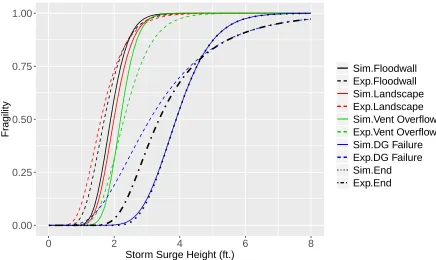
The same process can be extended to data-driven models and it should yield the same critical events as the one obtained based on simulation models for the validation study. In this case, the data-driven end state fragility is dependent on the data-driven DG failure event.

0.00 0.25 0.50 0.75 1.00

0 2 4 6 8

Storm Surge Height (ft.)

Fr

agility

Sim.Floodwall Exp.Floodwall Sim.Landscape Exp.Landscape Sim.Vent Overflow Exp.Vent Overflow Sim.DG Failure Exp.DG Failure Sim.End Exp.End

(58)

Validation Metric – Overlapping Coefficient

In the next step, multiple simulation fragility curves are generated by assuming a coefficient of variation of 0.1 for the simulation median capacity. Similarly, multiple data-driven fragility curves are generated by including data applicability as described in section II.4.2. Based on these multiple combinations of simulation and data-driven fragility curves, a histogram of overlapping coefficients is developed for all the top events as shown in Figure II.15. The OC for the system level has a mean of 0.59 which would be unacceptable if an acceptance criterion of 0.75 is adopted. Therefore, the overall validation has to be improved either by enhancing the simulation model or collecting additional experimental/field data for the DG failure event until the adequacy of the system level validation is satisfied.

Additional Data – Updating

(59)

0 2 4 6

0.00 0.25 0.50 0.75 1.00

Floodwall 0 1 2 3 4

0.00 0.25 0.50 0.75 1.00

Landscape 0 1 2 3 4

0.00 0.25 0.50 0.75 1.00

Vent Overflow 0.0 0.5 1.0 1.5 2.0 2.5

0.00 0.25 0.50 0.75 1.00

DG Failure

0 1 2 3

0.00 0.25 0.50 0.75 1.00

System−level (End State)

Overlapping Coefficient

Density

(60)

Table II.6: Additional Failure data of DG Failure event

Surge Height (ft.) No. of Failures Total Test Cases

3 5 50

4 28 50

5 45 50

6 49 50

0 5 10 15

0.00 0.25 0.50 0.75 1.00

Density

DG Failure

0.0 2.5 5.0 7.5 10.0

0.00 0.25 0.50 0.75 1.00

End State

Updating

After Before

Overlapping Coefficient

(61)

II.7 Summary and Conclusions

This paper presents a novel approach to quantitatively assess the system level validation by connecting individual validation events through a PRA informed validation framework. In this methodology, we include uncertainty in both simulation and data-driven models which gets reflected in the confidence levels of the overall validation. Event tree and fault trees are constructed for the system level performance, and they are mapped into a Bayesian network that allows propagation of fragility information from component level to system level. The uncertainty in the experimental data is represented in terms of three attributes: Relevance, Scaling, and Data Uncertainty. These attributes are graded based on their VUQ quality and are incorporated in the data-driven fragility analysis. In this study, the system level validation and the identification of critical events are evaluated based on fragility estimates. To improve the overall validation, we either enhance the simulation models of events along the critical path or collect additional field data until the adequacy of the system level validation is satisfied. This process helps in allocating the resources efficiently thereby reducing the effort to conduct high fidelity simulations and large-scale experiments. The proposed framework based on risk informed approach for system-level validation can be adopted by advanced flooding simulation codes such as Neutrino. The credibility of the Neutrino code for the intended application can be quantified similar to the synthetic example described in this manuscript.

The key conclusions of this study are summarized as follows:

(62)

• The basic events that are critical in the perspective of system level validation are identified.

• Multiple fragility curves are evaluated using different confidence levels instead of just the mean fragility curves.

• The credibility of the overall validation is estimated which gives confidence in the decision making.

(63)

PART III

Enhancement of Existing Risk Informed Validation

(64)

III.1 Introduction

In recent years, USNRC [32] and IAEA [33] have developed methodologies to assess the vulnerabilities of nuclear plants against site specific extreme hazards following the Fukushima-Daiichi nuclear accident. In many cases, advanced simulation tools are being considered to simulate multi-hazard, multi-physics, multi-scale phenomena and to evaluate vulnerability of nuclear facilities [13, 14, 15, 25, 27, 28, 30]. A knowledge about the accuracy of simulation codes is essential so that they may be used with confidence for decision making. The credibility of advanced simulation tools is assessed based on a formal verification, validation, and uncertainty quantification procedure. One of the key limitations in validation is the lack of relevant experimental data at system and sub-system levels. This limitation leads to decrease in confidence in the prediction of system-level risk and excessive reliance on expert opinion. Therefore, a robust validation framework is needed to formalize the confidence in predictive capability of advanced simulation results particularly in the context of uncertainties from various different sources.

(65)

However, these limitations can be addressed by implementing Bayesian network representation of PRA [13, 14, 15]. Only a few structures, systems and components (SSCs) at a nuclear plant are critical from a perspective of system-level safety or performance. Therefore, a validation framework that is based on a PRA informed approach is quite powerful by identifying the critical SSCs for validation and formalizing the confidence in prediction of system-level validation that are based on component level data.

(66)

for external hazards.

Recently, Kwag et al. [13] and Bodda et al. [14] proposed a PRA informed methodology for system-level validation within the context of uncertainty. In these methodologies, a Bayesian approach is used to assess the credibility of system-level estimates. Kwag et al. [13] used a seismic case study and Bodda et al. [14] a flooding case study to illustrate the application of the methodology. In these studies, the validation process is performed by creating a Bayesian network model to represent the system-level failure against an external hazard. Then, simulation based fragilities and data-driven fragilities (from experimental or high fidelity simulation data) are propagated in the Bayesian network model separately to evaluate the system-level fragility. The adequacy of the system-level validation is evaluated by comparing its simulation based and data-driven fragilities using a validation metric which is defined in terms of an overlapping coefficient. The validation process is carried out until the adequacy of system-level validation is satisfied against an acceptance criterion. However, the proposed risk-informed validation framework by [13] and Bodda et al. [14] have two key limitations:

(1) In the validation framework, the system-level fragility is obtained by propagating fragilities from basic events. Then, the validation metric is computed by comparing the simulation and data-driven fragilities. However, the system-level validation may actually give incorrect results if the set of critical events for simulation-based fragility differs from the set of critical events for data-driven fragility.

(67)

In this manuscript, we propose major enhancements to the existing framework for the assessment of decision regarding the adequacy of advanced simulation tools for system-level validation. Improvement in the PRA informed validation methodology requires development of additional attributes and a new set of validation metrics for a complete and wider applicability of the framework. The advantage of the proposed enhancements are illustrated in the context of the same examples as those used by Kwag et al. [13] in order to clearly delineate the proposed enhancements.

III.2 Summary of existing Risk Informed Validation framework by Kwag et

al. [13] and Bodda et al. [14]

The existing framework of Kwag et al. [13] and Bodda et al. [14] employs three key stages that are described below. The complete framework is illustrated through the flowchart shown in Figure III.1.

Stage 1:

(68)

Construct Event Tree/Fault Tree (ET/FT) corresponding to an initiating external hazard

Develop component level simulation fragility curves

Is mechanistic model to relate higher level nodes available? Determine

response surface

Map ET/FT into Bayesian Network (BN)

Evaluate fragilities for Intermediate event and Top event from simulation fragilties of components

Evaluate system risk/fragility and identify the most critical scenario Pick out important components

in identified critical path

Develop Assessment Base

• Identify experimental data at component and subsystem level

• Establish Relevance, Scaling, Uncertainty (R/S/U) Develop Data-driven Fragility

Curves by including R/S/U

Introduce overlapping coefficient (OC) as a validation metric

Use fragility data to calculate OC

If new data is available in any levels, update OCs of all levels based on the data

Decision (System OC>Criterion?)

System level validation process is done

Improve simulation or data-driven models

of components in identified critical path

(69)

Stage 2:

In Stage 2, an assessment base is developed which consists of experimental data at component and subsystem level. Next, a data-driven approach is adopted to quantify the quality of experimental data used for generating data-driven fragility curves. Similar to stage 1, system-level data-driven fragility curve is obtained by propagating data-driven fragilities from basic events through the Bayesian network.

Stage 3 and Decision:

In this framework, overlapping coefficient (OC) is used as the validation index to quantify the degree of validation within the context of uncertainty. OC is calculated by evaluating the percentage of overlapping area between two probability density curves and is given by Eq. (III.1). Numerically, OC ranges between 0 and 1. If OC = 0, then the distributions do not overlap with each other thereby indicating a complete disagreement and ifOC = 1, then the distributions are identical thereby indicating a perfect validation within the context of uncertainty.

OC =

∞

Z

−∞

min(fsim(y), fexp(y))dy (III.1)

For each event, based on the simulation and data-driven fragility curves, OC

(70)

III.2.1 Information needed to implement Risk Informed Validation

Framework for an external hazard scenario

The specific information required to carry out the validation of advanced simulation codes using the proposed validation framework is listed below:

• Develop event tree and its corresponding fault trees for the given external hazard scenario.

• For all the basic events or components, develop fragilities based on both simulation models and experimental or data-driven models. Establish the grade levels for Relevance, Scaling, and Data Uncertainty (R/S/U) for the available experimental data. The fragilities for each event can be developed based on individual simulation codes or an unified simulation code such as Neutrino can be used to evaluate fragilities for all the events at once.

However, in the initial development of risk informed validation methodology, it is possible that the experimental fragilities might not be available for some events or all the events. This is similar to initial implementation of PRA in 1970s when there was not much information available on fragilities of components. The initial implementation of PRA relied significantly on expert opinion. Similar expert-based knowledge can be used for the initial implementation of the proposed risk informed methodology. The framework can be used to determine which specific information is more critical and then as more information becomes available either through high fidelity simulations or experiments, the complete validation process can be refined.

(71)

• If the data-driven fragilities are not available for the non-critical events, then it is assumed that the data-driven fragilities are same as the simulation-based fragilities.

• For comparing the accuracy between simulation fragilities and data-driven fragilities, select overlapping coefficient (OC) as the validation metric. Additional validation metrics such as KL Divergence, Mutual Information, and Bayes Factor can also be selected.

• Represent the adequacy of the code for the intended application in terms of maturity levels as described in section III.6.

• Define acceptance criterion for system-level validation using expert judgment.

III.3 Critical Path in a Bayesian Network

Typically, only a few components or events are critical for the system-level failure in a nuclear power plant. Therefore, it is necessary to identify the events along the critical path that leads to a system-level failure. For identifying critical events in a logic tree, we can use the concept of importance measures. The importance measure of a basic event provides information about its impact on the system. There are different types of importance measures such as Fussell-Vesely (FV) Importance, Risk Reduction Ratio/Interval, Risk Increase Ratio/Interval, Criticality, and Birnbaum Importance that are used in decision-making process [35, 36, 37, 38]. FV importance provides information about the relative degree to which the basic event is contributing to the system failure probability. The F Vi for an eventi is defined as:

F Vi =

Pi

Psys

(72)

where Pi is the failure probability from all minimal cut sets which contains basic event i and Psys is the system failure probability.

Traditionally, the importance measures are evaluated only for fault tree analysis. As mentioned earlier, due to limitations of fault tree analysis, Bayesian networks are used in the risk informed decision making. Therefore, we extend the concept of importance measures to a Bayesian network. In this study, Fussell-Vesely (FV) Importance is employed for identifying the critical path because the FV importance provides relative importance of all the nodes in the Bayesian network whereas other importance measures provide information only about the basic events or root nodes [39, 40].

The extended definition [39, 40] of FV importance for any node (xi) in a Bayesian network can be obtained by evaluating the posterior failure probability of the node given that the system (φ) is failed,P(xi = 1|φ = 1).

F V(xi) =P(xi = 1|φ = 1) (III.3)

III.3.1 Illustrative Case Study: Seismic Risk of Failure in Building-Piping

System

(73)

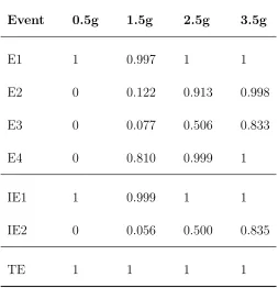
follow lognormal distribution. The lognormal fragility parameters of all the basic events are shown in Table III.1 and the intensity measure is taken as peak ground acceleration (PGA). The fault tree is mapped into a Bayesian network using a mapping algorithm [15] and the corresponding mapped Bayesian network is shown in Figure III.3. The critical path is obtained for different values of intensity measures as the failure probability of an event depends on the intensity measure. The FV importance measure for all the events (nodes) in the Bayesian network is computed using Eq. (III.3) for various intensity measures of 0.5g, 1.5g, 2.5g, and 3.5g (Table III.2) The critical path is identified based on a top-down approach and utilizing the FV importance measures. The required steps for obtaining the critical path are described below:

• Start with the top node (TE) in the Bayesian network and identify its parent nodes, Pa(TE) =IE1, IE2.

• Compare the FV importance measures for all the parent nodes and obtain the parent node with largest value. (IE1 = 0.999, IE2 = 0.056)

• Next, identify the parent nodes of node IE1 and similarly, obtain the parent node with largest value. (E1 = 0.997, E2 = 0.122)

• Repeat the process until the root node (basic events) is reached.

(74)

System Failure

Loss of Circulation

Excessive story drift of Bldg.

Safety-related equip. failure

Loss of Coolant

Support failure of piping

Leakage at joint of piping OR

OR AND

Figure III.2: Fault tree for Building-Piping System Failure

TE System Failure

IE1 Loss of

Circulation

E1

Excessive story drift of Bldg.

E2

Safety-related equip. failure

IE2 Loss of

Coolant

E3

Support failure of piping

E4

Leakage at joint of piping

(75)

Table III.1: Lognormal Fragility parameters of basic events

BASIC EVENT Median, ˆλ (g)

Log Standard

Deviation,βAU

E1. Excessive story drift of Building 0.75 0.35

E2. Safety-related equipment failure 1.9 0.25

E3. Support failure of piping 2.5 0.29

E4. Leakage at joint of piping 1.2 0.33

Table III.2: Fussell-Vesely Importance measure for Building-Piping System Failure

Event 0.5g 1.5g 2.5g 3.5g

E1 1 0.997 1 1

E2 0 0.122 0.913 0.998

E3 0 0.077 0.506 0.833

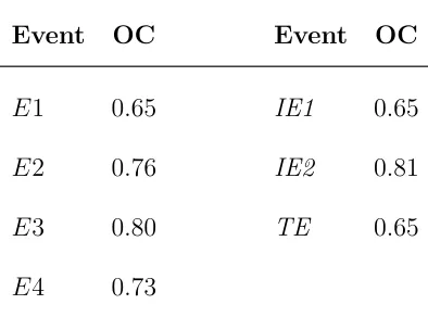
E4 0 0.810 0.999 1

IE1 1 0.999 1 1

IE2 0 0.056 0.500 0.835

(76)

III.4 Validation Path in a Bayesian Network

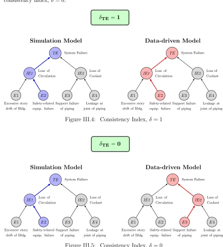
In the risk informed validation framework given by Bodda et al. [14], simulation and data-driven fragility curves for all the basic events in the fault tree and event tree are developed. Next, the fault trees and the corresponding event tree are mapped into a Bayesian network. The system-level fragilities are obtained by propagating fragilities from basic events through the Bayesian network. Based on the simulation and data-driven fragility curves, overlapping coefficient (OC) can be calculated for all the events. Then, the system-level OC is compared with a predefined acceptance criterion for validation. However, the validation may not be complete or consistent if the set of critical events for system-level simulation fragility differs from the corresponding set of critical events for system-level data-driven fragility. Therefore, in addition to OC, we employ Consistency Index (δ) in the validation metric in order to ensure that simulation and data-driven fragilities correspond to the same set of critical events.

III.4.1 Explanation of Consistency Index (δ)

(77)

consistency index, δ= 0.

Figure III.4: Consistency Index,δ = 1