Copyright 0 1994 by the Genetics Society of America
The Use of Mixture Models
to
Detect Effects of Major Genes on
Quantitative Characters in a Plant Breeding Experiment
Jiang Changjian,’ Pan Xuebiao and Gu Minghong
Department of Agronomy, Jiangsu Agricultural College, Yangzhou, 225001, People’s Republic of China
Manuscript received May 17, 1993 Accepted for publication September 24, 1993
ABSTRACT
An analysis based on Elston’s model of mixed major locus and polygenic inheritance is extended to include populations of progeny testing such as Fs, B1, and Bzs families derived from FZ and backcrosses in a cross between two inbred lines. Genetic hypotheses that can be validly tested by the likelihood ratio method in the analysis of a breeding experiment include homogeneity of variances due to environment and/or polygenes with transformable scale effect by Box-Cox power function, random and independent segregation of major genes, invariance of the effects of major genes with population types and additive and dominant models for polygenes. Testing hypotheses in the order suggested here can lead to a gradual simplification of the models and increases the feasibility of the subsequent analysis, but caution must be paid to the possible bias in parameter estimation and hypotheses tests. The procedure is applied to a set of data on plant height of rice with the effects of dwarf genes in crosses among three varieties. Two recessive dwarf genes are shown to be nonallelic and unlinked. One dwarf gene is shown to reduce plant height about 36-56 cm, and another 52-61 cm. The effect of polygenes, estimated as the standard deviation among possible inbred lines derived from these crosses, is about 11.7 cm. Interactions between the dwarf genes and the polygenic background are found, especially for one of the two genes. Both the polygenic effects and the interactions are much
-
smaller than the effects of the major dwarf genes.M
AJOR genes, traditionally related to qualitative characters, discussed in this study represent genes on quantitative traits with large effects relative to those detected only by means of genetic markers(GILBERT 1985a, 198513; JENSEN 1989; KNAPP, BRIDGES and BIRKES 1990; LANDER and BOTSTEIN 1989; SHRIMPTON and ROBERTSON 1988; PATERSON et al. 1988). Many economically important quantita-
tive characters including plant height (Gu, PAN and
LI 1986; Gu et al. 1988; HARGROVE 1979; NILAN 1964; PINTHUS and GALE 1990), pest and disease
resistance (SIMMOND 1979), and grain quality (KUMAR
and KHUSH 1987; MCKENZIE and RUTCER 1983; VA-
SEL 1975) in plant populations exhibit the effects of major genes. Separation of the effects of major genes and the effects of polygenes is important for under- standing the expression of a major gene in relation to polygenic background in genetics, and for predicting the segregation of a cross in breeding.
In plant breeding experiments concerning major genes, the important genetic information for a cross
may include the presence or the absence of a major
gene, dominance or recessivity of one allele to another at the major locus, the effects of the major gene as
well as polygenes, and possible comparisons between
different major genes. Given this type of information,
’
To whom correspondence should be addressed.Genetics 1 3 6 383-394 (January, 1994)
a breeding strategy for the use of the major gene
can be established. With mixture models, TAN and
D’ANGELO (1979) tried to estimate the numbers of major genes and polygenes responsible for the genetic
difference between two inbred lines by assuming equal
effects for each type of gene. Under the same struc-
ture ELSTON and STEWART (1973), ELSTON (1984)
and TAN AND CHANG ( 1 972) proposed several genetic models involving polygenes and/or major genes, and used the likelihood ratio test for comparisons among these models. More recently, it has been noted that
there are problems with the application of these meth-
ods, especially hypothesis tests, due to properties of
the likelihood method in mixture models (GOFFINET,
ELSEN and ROY and LOISEL 1992; HARTIGAN 1985; TITTERINGTON, SMITH and MAKOV 1985). To obtain reliable information necessary for assessment of the use of a major gene in a breeding program, we use ELSTON’S (1984) model of mixed major locus and
polygenes with modifications and extensions, and re-
strictions on hypotheses to be tested. Genetic hy-
potheses which we propose are about the homogeneity
of variances due to environment and/or polygenes in the presence of different major gene genotypes (with
transformation on observations when it is needed),
segregating ratios of genotypes of the major gene,
384 Jiang Changjian, Pan Xuebiao and Gu Minghong
T h e procedure is then applied to a set of data about
plant height of rice from an experiment which in-
volves two dwarf genes, one of which is widely used in many commercial varieties and the other is yet to
be explored. T h e comparison between two dwarf
genes could be important for the determination of the
value of the new gene in rice breeding, though its
effects on other traits need further study. Problems
about data transformation, progeny testing and as-
sumptions of homogeneous variances are further dis-
cussed. These problems are closely related to the
validity of the results from the analysis.
GENETIC MODELS AND STATISTICAL ANALYSIS
Consider a classical breeding program starting with
two inbred lines with genetic differences of major
genes as well as polygenes for a quantitative trait. Two
models and two population structures will be dis-
cussed. The first model involves one major locus with
six populations, the case considered by ELSTON ( 1 984),
two parents (PI and Pz), F1, F2, and two backcrosses
(BI and B2) distinguished in parameters by the sub-
scripts 1, 2 , 3, 4, 5 and 6 respectively. T h e second
model is an extension to two major loci which was also
considered by ELSTON without the effects of poly-
genes. T h e two models are then extended to include
families of progeny testing, such as Fa, B1, and B2,
derived from individuals of Fs, B1 and Bz, respectively, by self fertilization.
One-locus major gene model: Let the major gene
be denoted as A-a. For simplicity and for the applica-
tion in our example, we assume that A is dominant to
a (complete dominance or recessivity in major locus is commonly found in plant populations). Based on the phenotypes, the genotypic composition of the major gene for six populations are as follows
P1: aa P2: A A F1: AU
( 1 ) F2: 0 . 2 5 ~ 0 .
+
0.75A- B1: 0 . 5 ~ ~+
0 . 5 A a Bz: A-where A- represents Aa or AA. We denote this model
as Model 1.
If normality and additivity are assumed for the
effects of polygenes and environment (after transfor-
mation when needed), for each genotype of the major
gene the quantitative trait will have a normal distri-
bution with certain mean and variance. T h e PI, Pp, F1 and B:, populations are all composed of one single normal distribution, while the distribution of the trait
in the FP and B1 populations is a mixture of two normal
distributions. Let IJ and a2 represent the genotypic
means and variances of the major gene and subscripts
are used to make the distinction among different
populations and different genotypes from the same
population. Let
p
represent the mixing proportion insegregating populations. T h e joint log-likelihood is
then the sum of six functions shown in ELSTON (1 984)
and not repeated here.
Two-locus major gene model: Let the second locus
be represented by B-b. Complete dominance of B to b
and independent segregation of A and B are assumed.
Genotypic compositions of six populations are then PI: UUBB P2: AAbb F1: AaBb
F2: 0 . 0 6 2 5 ~ a b b
+
0.1875A-bb (2)+
0.18'75aaB-+
0.5625A-B-B1: 0.5aaB-
+
0.5AaB- B2: 0.5A-bb+
0.5A-Bb.T h e genotypes of PI and P2 may be aabb and AABB,
but the following analysis will not be affected. We will
call this Model 2 . In contrast to Model 1 , the distri-
bution of the trait in the F2 population now becomes
a mixture of four normal distributions and B2 is a
mixture of two. Mixing proportions in F2 are now
denoted as p41, p42, p43, p 4 4 , and in B1 and BZ as p51,
p 5 2 , and p61, p62, respectively. The log-likelihood func-
tion for Model 2 is obtained by the same way as for
Model 1 .
Compared to qualitative traits, F3 and similar pop- ulations may be even more important for the identi-
fication of genotypes of major genes for a quantitative
trait due to the additional effects of polygenes and
environment. In self-fertilized crops, Fs, B,, and Bzs
families are easy to obtain, and we extend the models to these families. T h e analysis of these families can also be combined with that of the above six popula-
tions, so w e discuss these families separately.
Models including
FS, B1.
andBZ.
families: T h e genotypic composition of the major genes and the likelihood functions for F3, B1, and Bz, are similar toeach other, so only the F3 family will be discussed in
detail.
Let m, represent the sample size in F3 family i.
Under Model 1 half of the families are homogeneous,
aa or AA, and the other half are heterogeneous. The
genotypic composition over all families with corre- sponding probabilities is
0.25aa, 0.25AA, 0.5(0.25aa
+
0.75A-) ( 3 )which will be called aa,
AA
and A a families, respec-tively. Individuals from the same F3 family are corre- lated due to a share of a proportion of polygenes. T o
formulate the likelihood function with this type of
family structure, ELSTON (1984) listed all possible
genotypic compositions in a sample. As the Fs family
size in plants is usually large, the method becomes
formidable here. Instead, we try a linear transforma-
tion. Let p denote the correlation coefficient in fami-
lies of (3). T h e transformation is then
"r
x-=alyy-a2yi, 'I j , = yV/mi, j = 1 ,
. .
.
,mi, (4)1 1 1
a1 = ___ a:!=--
-
j= 1
Detecting Effects of Major Genes 385
where y represents the original observations (assumed
to be normally distributed) and x the transformed
values which are uncorrelated with each other and
have the same variance as y. After transformation, the
means of x in aa and AA families are (a1
-
a2)p71 and(a1
-
(Y2)1172 where ~ 7 1 and p72 are genotypic means ofy for aa and AA over families. Two component means
for x in the mixture of Aa family are (alp71
-
( ~ 2 j i 7 )and (alp72
-
(YZC(7) where ji7 = 0.25p71+
0.75~72. T h eproof of these results is included in the APPENDIX.
Therefore the distribution of x is then a mixture of
three types of distributions due to the family, i.e. a
single normal distribution in aa and AA families, and
a mixture of two normal distributions in Aa family.
For k families the log-likelihood of x can be expressed
as
K +
c c
l n { E e x p (k mu -(xij
-
(a1-
aZ)p71)')i-1 j-1 2631,
+
- exp+
q73[& exp(
- ( X i j-
(alp71-
a 2 i 7 ) ) 2 q 7 2 (-(xij-
(a1-
a2)p72)'87% 2 &'2i
)
~ 7 1 , 2 d l i
)
+
-
p 7 z exp (-(Xij-
(alp72-
a&))')])W z i 2 4 ' 2 ,
k
-
c
In[a\m~"(al-
a2)]i= I ( 5 )
where q ' s are between family ratios and p's within
family ratios, and the last term is the Jacobian for the transformation. T h e within-family correlation coeffi-
cient p in the transformation of y to x is another
parameter like p and u2 in the model needed to be
estimated.
Under Model 1 the genotypic compositions of B1,
and BZs families are
BIS: O . ~ U U , 0.5(0.25aa
+
0.75A-);Bzs: 0 . 5 ( 0 . 2 5 ~ ~
+
0.75A-), 0.5AA.Within-family correlation and the component means can be defined in a similar way, as can the likelihood functions.
Under Model 2, nine types of F3 family can be
distinguished as
0.0625aabb, 0.0625AAbb,
0.0625aaBB, 0.0625AABB,
0.125(0.25aabb
+
0.75A-bb),0.125(0.25aabb
+ 0.75aaB-),
(6) 0.125(0.25AAbb
+
0.75AAB-),0.125(0.25aaBB
+
0.75A-BB),0.25(0.0625aabb
+
0.1875A-bb+
0.1875aaB-+
0.5625A-B-)which can be divided into three groups as homozy-
gote, single heterozygote and double heterozygote
families according to the genotypes of their parental
individuals in F2 generation. After the same transfor-
mation as (4), family means in the likelihood function
for the four homozygote families are
(a1
-
a2)p71, 1 = 1 , 2 , 39 4.T h e two component means in the mixture of A-bb
family are
alp71
-
f f 2 i 7 A 1 , alp72-
a2b7A1,where
F . 7 ~ 1 = 0.25p71
+
0.751172.Similar expressions exist for the other three single
heterozygote families. And for the double heterozy- gote family, the four component means are
alp71
-
a21171 1 = 1, 2 , 3, 47where
ji7 = 0.0625p71
+
O.1875p72+
0.1875p73+
0.56251174.All p's are defined over families and correspond to
the four groups of genotypes in (2). Then the distri-
bution of x is a mixture of nine types of distributions
due to the family, of which it is either a single normal
distribution or a mixture of two or four normal dis-
tributions. T h e log-likelihood function for F3 families
can be expressed as k m,
K
+
c c
I+[E
exp(
i=l j=1
2
du
)I
+ q 7 5 k exp
(
2 d l i
1
-(xij
-
(a1-
aZ)p71)'-(xij
-
( a l p 7 1-
aZi7.41))'+
-
expp 7 1 2
(
-(%j
-
(alp72-
aZi7A1))'6 7 % 2 d 2 i
)I
+ q7k. exp
(
-(xij-
(alp71-
a2i7B1))22~31,
)
+
p 7 2 2-
exp ( - ( X i j-
(alp73-
a 2 i 7 B 1 ) ) 26 7 %
2
d 3 i11
+
477b:
-
exp (-(xg-
( a l p 7 2-
aZi7A2))' 2 d z i1
+
-
expp 7 3 2
(
c74i 24'4,
11
-(xij
-
(alp74-
aZi7A2))'0741 2 4'4i
)I
+
4 7 8[t:
-
exp (-(xij-
( a l p 7 3-
a 2 i 7 B 2 ) ) 2+
p 7 4 2-
exp (-(%j-
( a l p 7 4-
(YZi7B2))'386 Jiang Changjian, Pan Xuebiao and Gu Minghong
h
where all parameters are defined corresponding to
genotypes in (6), and F A 1 and
FA2
are the means inA-bb and A-BB families,
FBI
and i i B 2 in aaB- andAAB-.
Genotypic compositions in B1, and BZs families are
BIS: 0.5(0.25aabb
+
0.75A-bb),0.5(0.25aaBb
+
0.75A-Bb);Bzs: 0.5(0.25aabb
+
0.75aaB-),0.5(0.25Aabb
+
0.75AaB-).T h e log-likelihood functions for B1, and B2, are similar to that of Fs, but simpler.
Likelihood-based technique for statistical analy- sis: As in ELSTON (1984) and TAN and D'ANGELO
(1 979) the following analysis will be used on the joint
log-likelihood function of all populations included in the experiment, and calculation depends heavily on
numerical methods. For estimation, the maximum
likelihood estimator (MLE) is to be used (TITTERING-
TON, SMITH and MAKOV 1985). T o obtain MLEs in
mixture models, the EM algorithm is often used in many situations. For details of the algorithm the
reader is referred to DEMPSTER, LAIRD and RUBIN
(1 977), REDNER and WALKER (1 984), and an applica-
tion can be found in BOOS and BROWNIE (1 991).
Under some restrictions on parameters, however, the maximization step in the EM algorithm won't have an
explicit solution (Boos and BROWNIE 1991). Other
numerical methods for this step or for the whole
estimation processes have to be used, such as Simplex
method or Powell's direction set method (PRESS et al.
1986). Though these methods may not be very effi- cient in multidimensional maximization, the second order derivatives of the log-likelihood function, which are often quite complicated, are not required.
For hypotheses testing, submodels of Model 1 and
2 derived from restrictions between parameters are
examined with standard likelihood ratio methods by
comparing -2 log A to a chi-square distribution with
appropriate degrees of freedom where A represents
the likelihood ratio. T h e genetic hypotheses consid- ered involve deviations in mixing proportions from some theoretical values and relative sizes of major gene effects. None of the hypothesis tests considered implies the collapse of two or more components into
one (see GHOSH and SEN 1985, and an application in
BOOS and BROWNIE 199 l), which will keep the validity
of a test from breakdown (HARTIGAN 1985; TITTER-
INGTON, SMITH and MAKOV 1985).
TESTING OF GENETIC HYPOTHESES
T h e following genetic hypotheses can be formu-
lated for the population structures with or without
progeny testing families.
Scale effect: T h e commonly used transformation to eliminate nonnormality in distribution and/or het- eroscedasticity in variances due to the same sources of variation for individuals from different groups is
the BOX-COX power function (Box and COX 1964).
For y
>
0, the BOX-COX transformation is given byy' =
[+
X # O ,l0gW X = O
where y' represents the transformed value. Many
kinds of dependence of the observational variations on the means, often called scale effects, can be ap- proximately corrected by this transformation. Special
values of X, such as 1/3, 1/2, are often used in genetic
analysis. For example WRIGHT (1968) used a log-
transformation to tomato fruit weight to obtain a good
fit to the assumed genetic model. Applications of the
transformation in mixture models can be found in
ELSTON (1984) and GRAY (1 992). With appropriate
choice of X value in the BOX-COX function, hetero-
scedasticity in variances due to the scale effect only implies that transformation will lead to
UT
= 6; = 63, 2 621 = 6 2 2 , = 6 2 2 (8)in Model 1 and
6: = 6; = 6:, 621= (J42 2 = 6 4 3 2 = 644, 2
2 2
6 5 1 = 6 5 2 , d l = d 2 (9)
in Model 2. For the F3 families it implies that all
genotypes of major genes in all families have the same variance, as do B1, and B2, families.
Under the hypothesis of homogeneity for variances,
the number of parameters in the models will be greatly
reduced, which makes the following analysis about the
mixing proportions and gene effects much easier. One
experiment, however, usually cannot provide enough
support for the comfortable use of this
type
of reducedmodels, and information from other experiments is required.
Segregating ratios for genotypes of major genes:
Inheritance of major genes for quantitative traits must
be determined to a great extent by genotypic ratios
in segregating populations, such as Fz, B1, B2, Fs, B1,
and B2, in addition to parents and F1 which are usually
taken as standard reference populations in analysis.
Gene actions to be identified include within locus as
well as between major gene loci, such as complete
dominance or recessivity, complementarity or repli-
cation, and linkage.
Random segregation in Model 1 represents
Detecting Effects of Major Genes 387
Additionally independent segregation in Model 2 im-
plies
p 4 1 = 0.0625, p 4 2 = p 4 3 = 0.1875,
p 4 4 = 0.5625, p 5 1 = p 5 2 = p 6 1 = p 6 2 = 0.5. (1 1)
For Fs, B1, and B2, families both between and within family ratios are informative, and the relative impor-
tance of the two may depend on the number of
families available and the size of each family.
Effect of major genes: T h e effect of a major gene
in Model 1 can be expressed as
d A = 1142
-
1141 = 1152-
~ 5 1 , (12)and in Model 2 as
d A = 1142
-
1141 1144-
1143 = 1152-
1151,d B = 1143
-
1141 = 1144-
1142 = 1162-
1161,assuming dA C dB. A similar relationship holds for Fs,
B1, and B 2 , .
T h e effect of a major gene represents the average difference among inbred lines derived from the cross.
Rejecting some of the equations in (1 2) or (1 3) may
suggest the presence of interactions between the ma-
jor gene and the polygenes (ELKIND and CAHANER
1986, ELKIND, CAHANER and KEDAR 1990). T h e ef-
fect of polygenes plays an important role in modifying
the phenotypes of major genes for many quantitative traits.
Effect of polygenes: T h e analysis of the polygenic
effect can be made by genotypic means as well as
variances in different populations similar to the tra-
ditional analysis of quantitative traits (MATHER and
JINKS 1982). When genotypic means are used for the
analysis, however, the effect of a major gene must be invariant with the population types. Using the geno-
typic means for the analysis after accepting (12) or
(13), additive and dominant models for polygenes
correspond to the following restrictions
(13)
Model 1
1141
+
31142 = 1 1 1+
112+
2113, 1151+
1152 = PI+
1139116 = (112
+
P s ) / ~ ,1142 = (1152
+
W6)/2,(14)
Model
2
1142
+
1143+
21144 = 1 1 1+
112+
2ps,1151
+
P52 = 11.1+
P39 P 6 l+
1162 = 112+
113,1144 = (1152
+
1162)/2.T h e complete additive model for polygenes must also have
P 4 2 = 113 and 1144 = P S .
Similar restrictions hold for Fs,Bl, and B2,.
In the analysis of variances, the polygenic genetic
variances in Fz, B1 and B2 can be estimated by sub-
tracting environmental variances estimated from
those of
P1,
P2
and F1. Let the environmental variancebe denoted as a: and variances in F 2 , B1 and B 2 as a:,
a; and af independent of major gene genotypes, and
additive and dominant components as D and H
(MATHER and JINKS 1982). T h e additive models for
polygenic effects imply
no matter whether Model 1 or Model 2 is used. T h e
additive-dominant models imply
Given the estimate of a:, equations in (1 5) provide a
one degree of freedom test for additive models with
only six families. Equations in (1 6) give the estimates
for D and H with no degree of freedom left for model
testing. Inclusion of F 3 , B1, and B 2 , will provide more
equations for estimation, and also some degrees of freedom for the test of the models.
ELSTON (1 984) proposed several symmetric restric-
tions which include the joint effect of major genes and
polygenes. For many plant traits, the effects of two
types of genes often follow different genetic models. Major genes are often nearly completely dominant or recessive and polygenes are from additive to partially dominant or recessive. Separate testing for their ef- fects are necessary for the determination of the use of the major genes in breeding, and also possible by the use of mixture models.
Testing hypotheses in the above order (scale effect, mixing proportions, effect of major genes and effect of polygenes) may gradually simplify the model, make the analysis become practically feasible, and also pro- vide later tests with significant meaning. For example,
only if (10) or (1 1) were accepted by testing, would
estimation and testing about the effect of the major gene become sound. Otherwise, an explanation must
be found for the rejection before further analysis can
be made. A type I1 error, however, might occur in
the primary test which would affect the following tests. If more than one family can provide information for testing the same genetic hypothesis in the analysis, the probability of a type I1 error is expected to be greatly reduced.
Comparisons between procedures of multiple test- ing: To investigate the possible effects of a type I1 error from the previous test on the subsequent tests, a simulation study was carried out to compare the
powers among a few testing procedures. Since the
tests about the effects of a major gene and polygenes
depend on the determination of the presence of the
major gene, we restricted the tests for segregating
388 Jiang Changjian, Pan Xuebiao and Gu Minghong
TABLE I
Power calculations at a = 0.05 for likelihood ratio tests in simulations
Hypothesis tested
True model & I = 0.25, P,I = 0.5 u: = u; = u:, UIpI = U L , UHI = uH2
d P. 1 P S I Test 1 Test 2 Test 3 Test 1 Test 2 Test 3
nl = nz = ns = 50, n4 = n5 = n6 = 200
3 0.2105 0.4444
3 0.2941 0.5556
4 0.2105 0.4444
4 0.2941 0.5556
3 0.2105 0.4444
3 0.2941 0.5556
4 0.2105 0.4444
4 0.2941 0.5556
nl = nn = ng = 100, n4 = ng = ng = 400
0.1 1 0.14 0.27 0.44
0.17 0.18 0.70 0.77
0.33 0.33 0.37 0.48
0.42 0.49 0.73 0.79
0.14 0.17 0.23 0.27
0.25 0.27 0.59 0.53
0.06 0.03 0.03 0.05
0.07 0.06 0.09 0.07
0.15 0.10 0.10 0.05
0.22 0.26 0.12 0.08
0.1 1 0.08 0.08 0.04
0.17 0.18 0.12 0.08
The true model is listed in the first columns, with the heading “d p41 p5]” indicating the distribution type under Model 1, major gene
effect, segregating ratios in Fn and B I populations. Two sets of values for p41 and p , , correspond to sI = 0.8, sz = 1, and sl = 1, sz = 0.8 with
p11 = o.25s1/(o.25s~
+
0.75s~), $51 = 0.5s1/(0.5sl+
0.5s~). Polygenic effects were generated by 10 independently segregated loci each withadditive effect of 0.7483 for the difference between two homozygotes. The environmental variance was assumed to be 0.3 in all cases. Two
sets of sample sizes were used and 100 samples were generated for each model. Testing procedures for Test 1, 2 and 3 are explained in the
text.
on variances (but a test for this is also needed) in the simulations. T h e purpose, however, is to shed light on tests about all hypotheses.
Model 1 with six families was used for the sample generation in the simulation. Ten independent loci with equal and additive effects were assumed for the
polygenes. Segregation of the ten loci may well ap-
proximate a normal distribution for a quantitative
trait. These genes were assumed to be evenly distrib- uted in two parental inbred lines with one major gene difference. T h e polygenic effects and environmental variation were chosen such that the variances within
major gene genotypes in F2 were one, which was used
as a standard to determine the magnitudes of the
major gene effects ( d ) . Measurements for individuals
in each family were obtained by assuming the effects of the major gene, polygenes and environments ran- domly generated with appropriate probability distri-
butions. Three testing procedures, which are ex-
plained next, were compared and EM algorithm was
used for the calculation in simulations. Results are
listed in Table 1.
Results in Table 1 show that for the test of segre-
gating ratios, simple tests (Test 1 , without assuming
heterogeneity for variances) usually have lowest power
when d = 3, and the two-step tests (Test
2,
assuminghomogeneous variances in the second test after the
first test accepted the hypothesis) always have the
highest powers. Test 3 is to take the joint tests for
variances and segregating ratios as a protection against
the reduction of the significance level, and only if the joint test is significant would the rejection of the
hypothesis be made by Test 1 or
2
(if Test 1 wassignificant, Test 3 was to reject the hypothesis other-
wise Test
2
was performed). T h e power of Test 3usually is higher than that of Test 1 when d = 3,
which is from the application of Test
2
when thehomogeneity of variances is not rejected by the first test. T h e differences in powers imply that in some
samples, though the joint tests are significant, neither
of the simple tests for segregating ratios and homo- geneity of variances is significant. But the results of
this comparison are reversed when d = 4. This may
partially reflect the complex relationship among the multiple tests.
Similar tests for homogeneity of variances were also performed in simulations though heteroscedasticity
was not used for generating the data. This is to be
used as a check for the actual significant level com- pared with nominal ones. T h e results of the tests do show differences in significant levels among three
procedures. Test 1 is the only one which gives right
significant levels. T h e increases in probabilities of false
rejection by Test 2 and 3 come from replacing sample
segregating ratios with theoretical mixing proportions after the acceptance of independent segregation by
the tests. As d = 4, however, this increase becomes
negligible.
T h e effects of the false assumption about homoge- neity of variances on tests of segregating ratios will be discussed later.
AN EXAMPLE: SEMI-DWARF GENES IN RICE
Semi-dwarf genes, briefly called dwarf genes, can
Detecting Effects of Major Genes 389
TABLE 2
Means and variances of plant height for three inbred lines of rice and 3 F1’s from these lines
Name Sample size Mean (cm) Variance (cm*)
NANJING 1 1 (PI) 60 105.04 16.38
YEZHILA (Pz) 59 109.47 28.72
NANJING 6 (Ps) 6 2 153.21 26.93
(PI X Ps)FI 77 145.33 28.01
(Pz X Ps)FI 49 168.85 70.61
(Pz X PI)FI 64 139.19 85.55
dwarf genes is relatively resistant to lodging and adap- tive to high fertility. Applications of these varieties greatly improved rice production, especially in South-
east Asia (HARGROVE 1979). It is known that variety
NANJING 1 1 (PI) carries the dwarf gene sd-1 widely
present in many commercial varieties, and the dwarf gene in another variety YEZHILA (Pz) with different
origin is to be explored. Three crosses were made
from the two and a tall parent NANJING 6 (Ps)
provided by our rice breeding program. Fifteen pop-
ulations (three parental lines, three Fl’s, and Fz, B1
and B2 populations derived from each cross) were
planted in a compact plot in 1992, and environmental
differences within the plot were expected to be very
small. Plant heights were obtained after all plants were
fully matured. Means and variances of P’s and Fl’s are
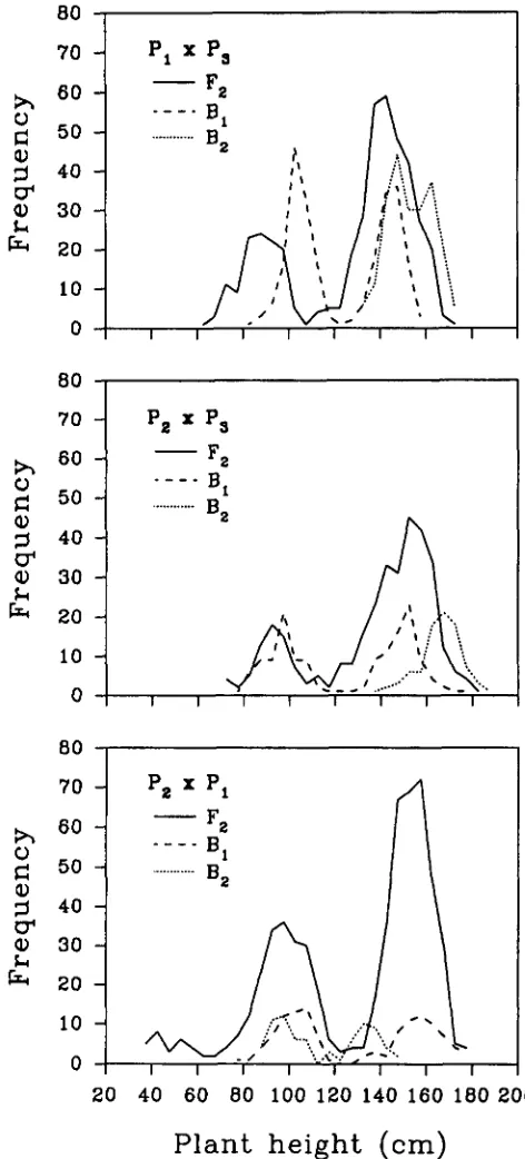
listed in Table 2 and distributions of Fz, B1 and B2
are in Figure 1 . Brief inspection of the table and the
figure reveals that the heights of both PI and Pz are mainly due to one recessive dwarf gene. Also the two dwarf genes appear to be nonallelic since, in addition
to the parental types in F2 of (Pz X PI), a large number
of tall plants and a group of shorter ones are present and are assumed to be nonhomozygotes and double homozygotes, respectively, for the two dwarf genes.
Then the Model 1 is used for the analysis of crosses
1 and 2, and the Model
2
for cross 3. T h e followinganalysis is based on the likelihood functions. Powell’s Direction Set method was used for the maximization, which worked quite well for our purpose.
Testing of scale effect and segregating ratios: At first, genotypic means and variances of dwarf genes and mixing proportions in all populations were esti-
mated without restrictions on parameters (except that,
in cross 3, heights of two semi-dwarf types in F2 are
SO close that distinction between them becomes im-
possible, so their variances are assumed to the same
as the tall type, which may be the best we can do in this situation). These estimates are intermediate re-
sults and not used in later analysis, so not listed here.
From the estimation, however, the genotypic variance of the tall type appeared to be greater than the semi- dwarf type in each of the segregating populations, which suggests the presence of scale effects. After the Box-Cox transformation is used, however, the likeli-
80
70
$
40301
k LQ 20
-
” ”50
40
30
20
10
0
70
h
6 od
500
$
40CY
P) 30
Ll LQ 20
10
0
-
20 40 60 80 100 120 140 160 180 200
Plant height
(cm)
FIGURE 1.-Distribution of plant height in the Fq, BI and Bz populations of three crosses derived from NANJING 1 1 (PI), YEZHILA (Pz) and NANJING 6 (Ps). Sample sizes in Cross 1 (PI X
Ps) are 437, 240, 215, in Cross 2 (Pp X Ps) 337, 147, 88, in Cross 3 ( P q X PI) 587, 122, 74.
hood ratio tests of homogeneity of variances are not
significant with the following exception (Table 3). In
Cross 3 (Pz X PI), the test is significant at 0.05 level
which is mainly due to the large difference in variances
of the two genotypes in B1 and in the variances of the two parents with about the same mean. Assuming the
value of X to be the average of the estimates in three
390 Jiang Changjian, Pan Xuebiao and Gu Minghong
TABLE 3
Statistical testing on heterogeneity of variances with the Box- COX transformation and segregating ratios of major genes in F2
and backcrosses for data in Table 1 and Figure 1
Cross Genetic hypothesis Result of test x * ~
1. PI X PS Homogeneity of variances"
(x
= 0.9387)bx;
= 1.16 Homogeneity of variances, X = 0.93 X: = 1.17Segregation at one locus
x%
= 2.352. PZ X Ps Homogeneity of variances
(x
= 0.8934) x% = 3.52 Homogeneity of variances, X = 0.93 x: = 3.58Segregation at one locus x% = 2.43
3. PZ X P I Homogeneity of variances
(x
= 0.9702) xi; = 8.97* Homogeneity of variances, X = 0.93 xi = 9.13 Independent segregation at two locix:
= 5.82a Homogeneity of variances represent uf = u; = uf, = &,
d l= u%2 in cross I , a: = u;, ,:a = u&, uzI = u& in cross 2, uf = u;,
ail u L , u%1 = &, u& = u& in cross 3.
*
X is MLE, and X = 0.93 the average of three estimates. * Significant at 0.05 level.the test may be approximately increased by one and tests in all 3 crosses are then not significant. Also, in
crosses 2 and 3, variances of F1 are unexpectedly much
greater than that of parents (the differences were
statistically significant by F tests, or equivalently by
likelihood ratio tests), and in cross 3 the same assump-
tion was used for the two semi-dwarf types in F2 as
stated above. Therefore the
'
x
tests have 4, 3 and 4degrees of freedom in crosses 1, 2 and 3, respectively,
when
X
= 0.93. T h e results in Table 3 also indicatethe absence of the possible incomplete recessivity of dwarf genes in FP, though more effective test for this hypothesis may need the progeny testing families.
In addition, tests show that segregation in crosses 1
and 2 is consistent with one completely recessive dwarf
gene difference, and in cross 3 with two unlinked
dwarf genes difference. Results are also listed in Table 3. Because of the large samples and the large effects of the dwarf genes, the reported results are not ex- pected to be due to this particular testing procedure which did make the analysis become much easier.
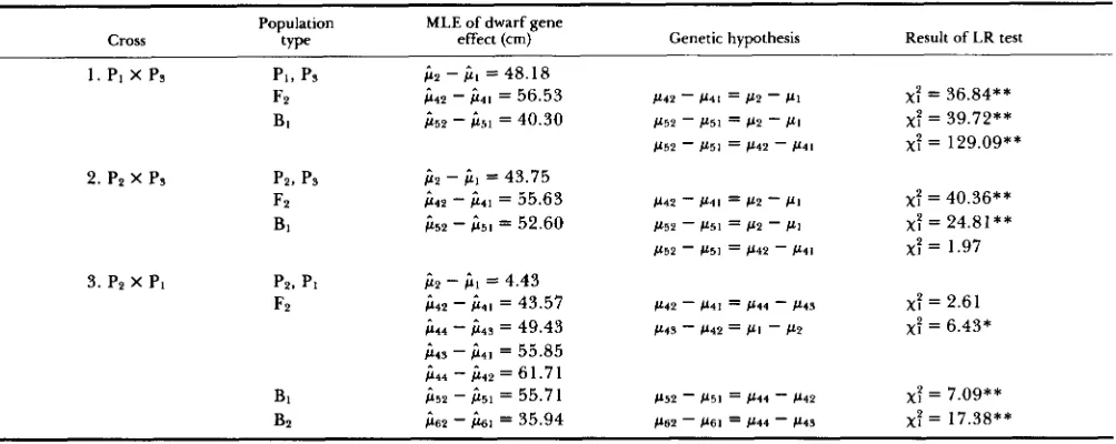
Hypothesis testing about effects of dwarf genes:
Estimates of the dwarf gene effects retransformed to the original scale and testing results about related genetic hypotheses are listed in Table 4.
T o test the difference of the dwarf gene effects in
F2 and in B1, MLEs were obtained with and without
the restriction of equality on gene effects respectively,
then the differences between the maximum likelihood
values were used for testing. In cross 1 the estimated
gene effect in Fz is significantly greater than that in
BI and both differ from the difference between two parents., In cross 2 no significant difference has been found between estimates from Fz and B1, but both
differ from the difference between parents. In cross
3 effects of two dwarf genes are additive in F2 but
different from those in B1 and Bz. Interactions be-
tween dwarf genes and polygenic background are
found. Differences between parents, one with a dwarf
gene and another with a normal gene, may include
additional effects of polygenes. From Table
4,
how-ever, the interactions are shown to be much smaller than the effects of dwarf genes in their magnitude.
Effect of polygenes: Because of the presence of interaction, genotypic means cannot be used to test the genetic model of polygenes. Based on variances,
the likelihood ratio tests for additive models (with
approximate chi square value 16.65, 0.034 and 10.67 in cross 1, 2 and 3, each with one degree of freedom) indicate the presence of nonadditive polygenic effect
in cross 1 and 3, but the absence in cross
2.
Additiveand dominant models could be used but cannot be tested due to the limited number of populations. For a rough estimation, the additive and dominant models were assumed and the corresponding components
were estimated. Results are listed in Table 5. T o
eliminate the effect of the Box-Cox transformation on estimates, variance components are presented rel- ative to that of the environment and the comparison between crosses then can be made. In Table 5 it is
shown that additive components may be the main
cause of the polygenic variation, and dominant com- ponents are relatively minor with two negative esti-
mates but these estimates might be biased in some
extent by the presence of epistatic effects.
T h e above results show that the effect of the dwarf
gene in NANJING 11 may change from 36 to 56 cm
with different genetic background, and in contrast the
effect of the dwarf gene in YEZHILA is more stable
with effect of 52 to 61 cm. On the average, the
additive component is about 5.7 times as large as
environmental variance. In the original scale the av-
erage variance of PI, P2 and PS is 24.1 cm2, so the
expected standard deviation due to polygenes in
inbred lines derived from these crosses will be about 1 1.7 cm, which is much less than the effects of major
dwarf genes. T h e effects of dwarf genes are so large
in this example that progeny testing families of Fs, B1,
and BZs seems to be unnecessary for detection.
DISCUSSION
Detecting major genes with large effects on quan- titative traits is very important in breeding programs. Genes with relatively small effects can be determined only by genetic markers and may be less useful than the major genes used in breeding programs by tradi-
tional methods for many quantitative traits. Except
for genes with very large effects (WELLER 1986,
1987), however, say six standard deviations of residual
Detecting Effects of Major Genes 39 1
TABLE 4
Estimates of the dwarf gene effects retransformed to the original scale and results of likelihood ratio (LR) tests for related hypotheses for data in Table 1 and Figure 1
Population
Cross
MLE of dwarf gene
t Y D e
,.
effect (cm) Genetic hypothesis .. Result of LR test1. PI x Ps PI, ps j i 2 - j i l = 48.1 8
F2 b 4 2
-
j i 4 1 = 56.53 P 4 2-
P 4 1 = @2-
PI x: = 36.84** BI 1152-
j i 5 1 = 40.30 P52 - b5l = 112-
PIx:
= 39.72**P52
-
1151 = P 4 2 - P4lx:
= 129.09** 2. P2 x Ps PZ, ps+
- j i ] = 43.75F2 c(1p
-
& I = 55.63 b 4 2-
P4l = c(2-
PIx:
= 40.36** BI i 5 2-
j i 5 1 = 52.60 P52 - P51 = PP-
PI x: = 24.81**P52
-
c(5l = P 4 2 - P 4 1 x: = 1.973. P p x PI PP, PI );2
-
j i I = 4.43FP i 4 2
-
c(41 = 43.57 P42 - P41 = 1144-
P 4 Sx:
= 2.61ji14
-
i i 4 s = 49.43 114s-
1142 = P I - P2 x: = 6.43*j i 4 3 - j i 4 1 = 55.85 j i 4 4
-
);42 = 61.71BI j i 5 2 - );51 = 55.71 1152
-
P 5 1 = P 4 4-
P 4 2 x: = 7.09** BP );62-
);61 = 35.94 P62 - P 6 1 = b 4 4-
C(4S x: = 17.38**Significant at the * 0.05 and ** 0.01 level.
TABLE 5 are used. Differences between genotypic variances of
Approximate estimates of additive (D) and dominant (H) components of polygenic variances relative to that of environment (V.) for data in Figure 1 after the BOX-COX
transformation with X = 0.93
Cross
Additive component Dominant component
(D/Ve) ( W J J
~ ~
1. PI x Ps 6.50 0
2. P2 x Ps 8.35 0
3. Ps x PI 2.25 3.85
I
major genes in segregating populations, however, are less likely influenced by factors other than scale effect and these variances are relatively large in magnitude.
So, estimating X by including segregating populations
may be more reliable, though the calculation is usually more difficult due to large sample size.
Progeny testing: With progeny testing the detec- tion of major gene effects can be based on within as well as between family variation. First, analysis can be
. -
Let V(F?), V(B1) and V(B2) represent the genotypic variances in carried out by the comparison of means and variances
Fz, BI and BZ respectively. D = 4([V(Fp)
-
(V(B,)+
V(Bp))/2], H = among fami1ies (Mo HUIDoNG'
993). Under Mode14[V(F2)
-
D/2-
Vel. V. is the average variance of p I , P ~ , pS and 1, means and variances of aa, Aa and AA families inFI(PI X Ps), which showed homogeneous variances by testing, and Fs are
equals 13.77 cm2.
Family aa Aa AA
the size of each population and deviations from the model assumptions, which are briefly discussed next.
Mean p;, 0 . 2 5 ~ ;
+
0 . 7 5 ~ ; &,Variance a2 0.1875d2
+
a2' a2Estimation of scale effect: If the heteroscedasticity
in variances due to the same sources of variations,
environment and/or the same group of polygenes, is mainly from the scale effect, the power function may be the right choice of the transformation for a wide range of quantitative traits, and the mixture model will be greatly simplified (though there may be nu- merical difficulties associated with the estimation of X, see GRAY, 1992). ELSTON (1984) suggested that an
estimate of X can be obtained from parents and F1,
and then used in the analysis of Fz, B1 and Bz. Our
experience indicates that variation in parents and F1 is often influenced by factors other than scale effect, such as purity of parents, stability differences between parents and F1. Also variation in these populations is relatively small, a slight disturbance may have large
effect on the estimation of X if only these populations
where the prime is to denote the average effects in
the progeny generation, d = P;
-
P;. Differencesbetween means and/or variances are then an indica- tion of the presence of a major gene. Detailed analysis is to be made on the likelihood function. The same procedures can be used for B1, and Bzs, and Model 2 as well.
Assumption about homogeneity of variances:
Though the hypothesis of homogeneity of variances
can be tested, false hypotheses often cannot be re-
jected due to the limited sample size. Then the as-
sumption may lead to a gain in the efficiency of MLE when the assumption is true, or a loss in the bias when
it is false. T h e following discussion for these two
aspects will depend on some numerical calculations
(for more discussions see GRAY 1992).
392 Jiang Changjian, Pan Xuebiao and Gu Minghong
TABLE 6
Asymptotic variances of MLE values of p and d when equal variance is correctly assumed, as u: = uz = 1, pI = 0 , and the
values of p2 and p vary
P
I r s 0.25 0.5
v a r ( i ) (relative efficiency)
2 1.49 (14.40) 1.36 (16.94)
3 0.32 (2.59) 0.39 (2.50)
4 0.21 (1.15) 0.28 (1.13)
2 13.07 (10.81) 9.27 (1.00)
3 7.18 (2.00) 4.63 (1.00)
4 5.92 (1.13) 4.11 (1.00)
Var(ci) (relative efficiency)
The relative efficiencies (in parentheses) of the estimates without assuming equal variances.
gating ratios in FZ and B1 be represented by
p
= 0.25and
p
= 0.5 respectively. T h e numerical analysis isbased on data generated by the following way intro-
duced by GRAY (1992) with some changes. T h e
PROBIT function in SAS (1 988) is an inverse normal
distribution function. T o obtain n observations with
p
= 0.25, let xi = PROBIT(ui)al+
pl with ui = (2i-
1)/0.5n, i = 1,
. . .
, 0.25n assuming 0.25n to be aninteger, and similarly xj = PROBIT(uj)az
+
pz withu , = ( Z j - 0 . 5 n - 1 ) / 1 . 5 n , j = 0 . 2 5 n + 1 , .
. .
, n . D a t a produced in this way may be thought of as a nearly perfect sample in the sense that the number of obser- vations in any interval is proportional to the probabil-ity under the true mixture density. T h e numerical
results from these data for large n will be close to the theoretical limits which are not available by analytical
methods. Asymptotic variances of MLEs are calcu-
lated with Fisher’s information matrix.
In the numerical calculations, we assumed n = 2000,
p1 = 0 and a: = 1 and let
p ,
pz and a4 vary. Majorgene effect is represented by d = ~2
-
~ 1Results are .listed in Table 6 and Table
7.
Table 6 shows that ifthe equal variance assumption is true, estimation of
p
and d with the restriction is much more efficient than
that without it. T h e relative efficiency (represented
by the ratio of the inverses of variances) is about 14
and 1 1 for estimates of
p
and d when the true d equals2, but only slightly bigger than 1 when d = 4. In
Table 7 estimation is made by assuming homogeneity
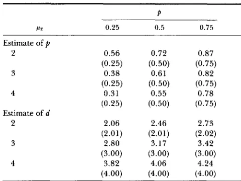
when two variances are actually not equal. In all cases considered, the estimates are biased. T h e most serious
bias happens when d equals 2, and it is reduced as the
value of d increases. As a check, the estimates without the restriction are also given in the table, which shows
that the MLE is asymptotically unbiased if the right
model is specified.
A trade-off exists between efficiency and possible bias of MLE when homogeneity in variances is un-
known, the sample size is only moderate and the effect
TABLE 7
Asymptotic limits of estimation of p and d when equal variances incorrectly assumed as p, = 0, U; = 1, U ; = 2 and the
values of p2 and p vary for the true parameter values
P
P? 0.25 0.5 0.75
Estimate of p
2 0.56 0.72 0.87
(0.25) (0.50) (0.75)
3 0.38 0.61 0.82
(0.25) (0.50) (0.75)
4 0.31 0.55 0.78
(0.25) (0.50) (0.75)
2 2.06 2.46 2.73
(2.01) (2.01) (2.02)
3 2.80 3.17 3.42
(3.00) (3.00) (3.00)
4 3.82 4.06 4.24
(4.00) (4.00) (4.00) Estimate of d
The corresponding limits without assuming equal variances are included in parentheses.
of major gene is not very large relative to that of
polygenes and environment. T h e efficiency in MLE closely relates to the efficiency of hypothesis testing
by likelihood ratio method. So this trade-off also exists
for hypothesis testing. These results are comparable
with the results in Table 1 from simulations.
GRAY (1992) pointed out that there is a certain
amount of non-identifiability between X and two var-
iances under Model 1. With the Box-Cox transfor-
mation, component distributions in the mixture will change differently, then the real differences in com- ponent variances could be disguised by a false choice
of the value of X when the genetic models are deter-
mined by the result of the statistical test in one exper-
iment. Then if an estimate of X can be appropriately
obtained in the analysis, the equal variance assumption would increase the efficiency of the estimation and
hypothesis testing. If the estimate of X has large error
in it, bias in the analysis will occur. A precise estimate
of X may depend on the analysis of the results from
more than one experiment.
The authors wish to thank MO HUIDONG for much critical advice;
DENNIS D. Boos, CAVELL BROWNIE and GERRY GRAY for their
valuable discussions; B. S. WEIR for the great patience he showed
when he edited the manuscript; and several anonymous reviewers
for comments on earlier drafts of the manuscript.
LITERATURE CITED
Boos, D. D., and C. BROWNIE, 1991 Mixture models for contin-
uous data in dose-response studies when some animals are
unaffected by treatment. Biometrics 47: 1489-1504.
Box, G . E. P., and D. R. Cox, 1964 An analysis of transforma-
tions. J. Royal Stat. Society B 26: 21 1-252.
DEMPSTER, A. P., M. N. LAIRD and D. B. RUBIN, 1977 Maximum
likelihood from incomplete data via the EM algorithm. J. Royal
Detecting Effects of Major Genes 393
ELKIND, Y., and A. CAHANER, 1986 A mixed model for the effects
of single gene, polygenes and their interaction on quantitative
traits. 1. The model and experimental design. Theor. Appl.
Genet. 72: 377-383.
ELKIND, Y., A. CAHANER and N. KEDAR, 1990 A mixed model
for the effects of single gene, polygenes and their interaction
on quantitative traits. 2. The effects of the nor gene and
polygenes on tomato fruit softness. Heredity 64: 205-213.
ELSTON, R. C., 1984 The genetic analysis of quantitative trait
differences between two homozygous lines. Genetics 108: 733-
744.
ELSTON, R. C., and J. STEWART, 1973 The analysis of quantitative
traits for simple genetic models from parental, F, and backcross
data. Genetics 73: 695-7 1 1.
GHOSH, J. K., and P. K. SEN, 1985 On the asymptotic performance
of the log likelihood ratio statistic for the mixture model and
related results, pp. 789-806, in Proceedings of the Berkeley
Conference in Honor of Jerry Neyman and Jack Kiefer, edited by
L. M. LE CAM, and R. A. OLSHEN, Vol. 2, Wadsworth, Pacific
Grove, CA.
GILBERT, D. G., 1985a Estimating single gene effects on quanti-
tative traits. 1 . A diallel method applied to Est 6 in D. melano-
gaster. Theor. Appl. Genet. 69 625-629.
GILBERT, D. G., 1985b Estimating single gene effects on quanti-
tative traits. 2. Statistical properties of five experimental meth-
ods. Theor. Appl. Genet. 69: 631-636.
GOFFINET, B., J. M. ELSEN and P. LE ROY, 1990 Statistical tests
for identification of the genotype at a major locus of progeny-
tested sires. Biometrics 46: 583-594.
GRAY, G., 1992 Bias in misspecified mixtures, in Institute of statis-
tics series 2227, North Carolina State University.
Gu MINGHONG, PAN XUEBIAO and LI X I N , 1986 Inheritance
analysis of major varieties of rice cultivated in Southern China.
Sci. Agric. Sin. 19(1): 41-48.
Gu MINGHONG, PAN XUEBIAO, LI XIN and DONG GUICHUN,
1988 A new semi-dwarf germplasm isolated from dwarf va-
riety and its genetic identification in Oryza sativa L. SUBSP.
HSIEN. Sci. Agric. Sin. 21(1): 33-40.
HARTIGAN, J. A., 1985 A failure of likelihood asymptotics for
normal mixtures, in Proceedings of the Berkeley Conference in
Honor ofJerry Neyman and Jack K e f e r , edited by L. M. LE CAM
and R. A. OLSHEN, Vol. 2. Wadsworth, Pacific Grove, CA.
HARGROVE, T. R., 1979 Diffusion and adoption of semi-dwarf
rice cultivars as parents in Asian rice breeding programs. Crop
Sci. 19(5): 571-574.
JENSEN, J., 1989 Estimation of recombination parameters between
a quantitative trait locus (QTL) and two marker gene loci.
Theor. Appl. Genet. 78: 613-618.
KNAPP, S. J., W.
c.
BR1DCE.S JR. and D. BIRKES, 1990 Mappingquantitative trait loci using molecular marker linkage maps.
Theor. Appl. Genet. 79: 583-592.
KUMAR, I., and G . S. KHUSH, 1987 Genetic analysis of waxy locus
in rice (Oryza sativa L.), Theor. Appl. Genet. 73: 481-488.
LANDER, E. S., and D. BOTSTEIN, 1989 Mapping Mendelian fac-
tors underlying quantitative traits using RFLP linkage maps.
Genetics 121: 185-1 99.
MCKENZIE, K. S . , and J. N. RUTGER, 1983 Genetic analysis of
amylose content, alkali spreading value and grain dimension in
rice. Crop Sci. 23: 306-313.
MATHER, K . , and J. L. JINKS, 1982 Biometrical Genetics (3rd ed.),
Chapman and Hall Ltd.
MO HUIDONC, 1993 Genetic analysis of quantitative traits. Acta
Agron. Sin. 19(1): 1-6.
NILAN, R. A., 1964 The cytology and genetics of barley 1951-
1962, pp. 1-278, in Monographic supplement No. 3 vol. 32 No.
1 , Washington State Univ. Press.
PATERSON, A. H., E. S. LANDER, J. D. HEWITT, S. PETERSON, S. E.
LINCOLN and S. D. TANKSLEY, 1988 Resolution of quantita-
tive traits into Mendelian factors by using a complete linkage
map of restriction fragment length polymorphism. Nature 335:
721-726.
PINTHUS, M. J., and M. D. GALE, 1990 The effect of "gibberellin-
insensitive" dwarfing alleles in wheat on grain weight and
protein content. Theor. Appl. Genet. 79: 108-1 12.
PRESS, W. H., B. P. FLANNERY, S. A. TEUKOLSKY and W. T.
VETTERLING, 1986 Numerical recipes. Cambridge University
Press, Cambridge.
REDNER, R. A., and H. F. WALKER, 1984 Mixture densities,
maximum likelihood and the EM algorithm. SIAM Rev. 2 6
195-239.
SAS, 1988 SAS Language Guide, Version 6.03 Edition. SAS Institute Inc., Cary, NC.
SHRIMPTON, A. E., and A. ROBERTSON, 1988 The isolation of
polygenic factors controlling bristle score in Drosophila mela-
nogaster. I . Allocation of third chromosome sternopleural bris-
tle effects to chromosome sections. Genetics 118: 437-443.
SIMMONDS, N. W., 1979 Principles of crop improvement, pp. 67-70,
270-274, Longman Inc., New York.
TAN, W. Y., and W. C. CHANG, 1972 Convolution approach to the genetic analysis of quantitative characters of self-fertilized
populations. Biometrics 2 8 1073-1 090.
TAN, W. Y., and H. D'ANGELO, 1979 Statistical analysis of joint effects of major genes and polygenes in quantitative genetics.
Biomet. J. 21: 179-192.
TITTERINGTON, D. M., A. F. M. SMITH and U. E. MAKOV,
1985 Statistical analysis of finite mixture distributions. Wiley,
New York.
VASEL, S. K., 1975 In Proceedings of the CIMMYT-Purdue Sympo-
sium on Protein Quality in Maize, pp. 197-2 16. Dowden, Hutch-
inson & Ross, Inc., New York.
WELLER, J. I., 1986 Maximum likelihood techniques for the map-
ping and analysis of quantitative trait loci with the aid of genetic
markers. Biometrics 42: 627-640.
WELLER, J. I., 1987 Mapping and analysis of quantitative trait loci
in tomato with the aid of genetic markers using approximate
maximum likelihood methods. Heredity 59: 41 3-421.
WRIGHT, S., 1968 Evolution and the Genetics of Populations, Val. I .
Genetic and Biometric Foundations. University of Chicago Press, Chicago.
Communicating editor: B. S. WEIR
APPENDIX
Linear transformation to eliminate within family correlation: Model 1 is assumed for the proof and the
result can also be applied to Model
2.
Let m be thesample size in a F3 or BI, family. In matrix notation,
observations on individuals, transformed for scale ef-
fect if necessary, are denoted by the n X 1 column
vector Y. Then the distribution of Y may be repre-
sented as (pointed out by one reviewer)
Y = BY,
+
(I-
B)Y2,where Y1 is MVN(p,,l, Z), Y 2 is M V N ( P , ~ I , Z) (MVN
denotes the multivariate normal distribution with cer-
tain mean and covariance matrix), B is diagonal with
diagonal element Bi, independent and identically dis- tributed Bernoulli random variable, I identity matrix
and 1 an n x 1 vector with all 1 's, and Z has all
diagonal elements as u2 and all off-diagonal elements
394 Jiang Changjian, Pan Xuebiao and Gu Minghong
LetZ" be decomposed asZ" = a"2R"1/2.R-1/2 *B Y
the result in ELSTON (1984) it is easy to check that the
form of R-1'2 is also a symmetric matrix with all
diagonal elements as
1
y1 =
+
(m-
1)m J 1
+
(m-
1)p mJ1'"p'and all off-diagonal elements as
1 1
7 2 =
m J 1
+
(m-
1)p m-'-
Let a1 = y1
-
72, ap = -myz, that is1 1 1
ff] =
-
ffz=--&' J 1
+
(m-
1)p'W h e n r n , 2 a n d O ~ p < l , a l a n d a 2 ~ 0 .
Let X = R"l2Y. Since both B and R-'12
are symmetric, R"l2B = BR-'/' and R""(1
-
B) =(I
-
B)R"/'. Then we haveX = R"'2BYI
+
R"/'(I-
B)Y2= B R - ~ / ~ Y ~
+
(I-
B ) R - ~ / ~ Y ~= BXI
+
(I-
B)X2where X1 is MVN(pxl 1, a21,), and X2 MVN(px21, u21,),
that is, the distribution of the element of X is a
mixture of two normal distributions, similar to Y but
means have changed. Over families pxl and px2 for
genotypes aa and A- will equal (YIP71
-
~ y z j i 7 andf f 1 p 7 2