To Carry out Analysis of Natural Convection over a Flat Plate

(1)

To Carry out Analysis of Natural Convection

over a Flat Plate

S.Nakkeeran

2

, Geeta Sagolshem

1

, Dr. J. Hameed Hussain

3

Assistant Professor, Department of Mechanical Engineering, Bharath University. Chennai, India M.Tech, Department of Thermal Engineering, Bharath University, Chennai, India Professor, Department of Mechanical Engineering, Bharath University, Chennai, India

ABSTRACT: This project combines many different sources in the field of heat transfer. Its purpose is to collect and organize the laminar heat transfer principles that are fundamental to heat transfer textbooks. The ultimate aim of the project is to examine the natural convection co-relation, at the atmospheric boundary layer flow of viscous fluid along a hot flat plat as well as the effect of Reynolds Number, Prandtl Number on heat transfer co-efficient i.e. Grashoff Number for flow over the flat plate. In addition the local Grashoff number are obtained, which can be used in estimation of flow and heat transfer performance over a flat plat locally.

I.INTRODUCTION

Heat can be defined as the form of energy that can be transferred from one system to another as a result of temperature difference. A thermodynamic analysis is concerned with the amount of heat transfer as a system undergoes a process from one equilibrium state to another. The science that deals with the determination of the rates of such energy transfers is the heat transfer. The transfer of energy as heat is always from the higher-temperature medium to the lower-temperature one, and heat transfer stops when the two mediums reach the same lower-temperature.

Heat can be transferred in three different modes: conduction, convection, and radiation. All modes of heat transfer require the existence of a temperature difference, and all modes are from the high-temperature medium to a lower-temperature one. In modes of heat transfer and their types (conduction, convection & radiation) it is discussed on basis of the boundary layer on thermal and velocity, which is of great importance and for understanding of heat transfer.

This chapter mainly focus on the mechanism of convection based on forced and nature/free convection i.e. their physical interpretation, governing equations and their dimensionless parameter over a flat plate.

II.MECHANISM OF CONVECTION

Consider the cooling of a hot block by blowing cool air over its top surface (Fig.2.1.1). Energy is first transferred to the air layer adjacent to the block by conduction. This energy is then carried away from the surface by convection, that is, by the combined effects of conduction within the air that is due to random motion of air molecules and the bulk of macroscopic motion of the air that removes the heated air near the surface and replaces it by the cooler air.

Heat transfer processes that involve change of phase of a fluid are also considered to be convection because of the fluid motion induced during the process, such as the rise of the vapor bubbles during boiling or the fall of the liquid droplets during condensation. Despite the complexity of convection, the rate of convection heat transfer is observed to be proportional to the temperature difference, and is conveniently expressed by Newton’s law of cooling as

(2)

where h is the convection heat transfer coefficient in W/m2°C or Btu/h · ft2 · °F, As is the surface area through which convection heat transfer takes place, 𝑇𝑠 is the surface temperature, and 𝑇∞ is the temperature of the fluid sufficiently

far from the surface.

The convection heat transfer coefficient h is not a property of the fluid. It is an experimentally determined parameter whose value depends on all the variables influencing convection such as the surface geometry, the nature of fluid motion, the properties of the fluid, and the bulk fluid velocity.

2.1 Forced Convection

Forced convection is the transfer of heat by convection in which the relative velocity is created by some outside source. For instance, a fan blowing air over a plate is forced convection. Any time there is a free stream velocity, there is going to be forced convection.

Common Classification of Convection:-

A. Based on geometry: External flow / Internal flow

B. Based on driving mechanism: Natural convection / forced convection / mixed convection C. Based on number of phases: Single phase / multiple phases

D. Based on nature of flow: Laminar / turbulent

2.1.1 Over A Flat Plate

An internal flow is surrounded by solid boundaries that can restrict the development of its boundary layer, for example, a pipe flow. An external flow, on the other hand, is flow over bodies immersed in an unbounded fluid so that the flow boundary layer can grow freely in one direction. Examples include the flows over airfoils, ship hulls, turbine blades, etc.

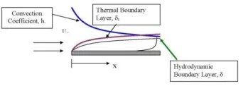
Fig.2.1.1 Internal and External flows on the boundary

Fluid particle adjacent to the solid surface is at rest. These particles act to retard the motion of adjoining layers boundary layer effect inside the boundary layer.

2.1.2 Forced Convection Correlations

Since the heat transfer coefficient is a direct function of the temperature gradient next to the wall, the physical variables on which it depends can be expressed as follows:

h=f (fluid properties, velocity field, geometry, temperature etc.)

(3)

Forced convection: Non-dimensional groupings

 Nusselt No. Nu= hx / k = (convection heat transfer strength)/ (conduction heat transfer strength)

 Prandtl No. Pr =v/α = (momentum diffusivity)/ (thermal diffusivity)

 Reynolds No. Re = U x / v = (inertia force)/(viscous force)

 Viscous force provides the dampening effect for disturbances in the fluid. If dampening is strong enough => laminar flow

 Otherwise, instability => turbulent flow => critical Reynolds number For forced convection, the heat transfer correlation can be expressed as Nu=f (Re, Pr)

The convective correlation for laminar flow across a flat plate heated to a constant wall temperature is:

Fig.2.1.2 Laminar flow over the flat plate

𝑁𝑢𝑥 = 0.323.𝑅𝑒𝑥

1 2. 𝑃𝑟13

Where, 𝑁𝑢𝑥 = h.x/

𝑅𝑒𝑥 = (𝑈∞.X.ρ)/µ

Pr =𝑐𝑝. µ/k

2.1.3 Physical Interpretation Of Convective Correlation

The Reynolds number is a familiar term to all of us, but we may benefit by considering what the ratio tells us. Recall that the thickness of the dynamic boundary layer, is proportional to the distance along the plate,

𝑅𝑒𝑥 = (𝑈∞.X.ρ)/µ α (𝑈∞. δ. ρ)/µ = (ρ.𝑈𝑥2) / (µ. 𝑈∞/δ)

The numerator is a mass flow per unit area times a velocity; i.e. a momentum flow per unit area. The denominator is a viscous stress, i.e. a viscous force per unit area. The ratio represents the ratio of momentum to viscous forces. If viscous forces dominate, the flow will be laminar; if momentum dominates, the flow will be turbulent.

2.1.4 Physical Meaning Of Prandtl Number

The Prandtl number was introduced earlier. If we multiply and divide the equation by the fluid density, ρ, we obtain:

Pr = (µ/ρ)/ (k/ρ.𝑐𝑝 = υ/α

(4)

δ/𝛿𝑡 = 𝑃𝑟

1 3

2.1.5 Physical Meaning Of Nusselt Number

The Nusselt number may be physically described as well.

𝑁𝑢𝑥 = h.x/k

If we recall that the thickness of the boundary layer at any point along the surface, is also a function of x then

𝑁𝑢𝑥 α h. δ/k α (δ/k.A)/ (1/h.A)

It is seen that the Nusselt may be viewed as the ratio of the conduction resistance of a material to the convection resistance of the same material.

Students, recalling the Biot number, may wish to compare the two so that they may distinguish the two.

𝑁𝑢𝑥 = h. x/𝑘𝑓𝑙𝑢𝑖𝑑

𝐵𝑖𝑥 = h. x/𝑘𝑠𝑜𝑙𝑖𝑑

The denominator of the Nusselt number involves the thermal conductivity of the fluid at the solid-fluid convective interface; the denominator of the Biot number involves the thermal conductivity of the solid at the solid-fluid convective interface.

2.1.6 Local Nature of Convective Correlation

Consider again the correlation that we have developed for laminar flow over a flat plate at constant wall temperature

𝑁𝑢𝑥 = 0.323𝑅𝑒𝑥

1 2_.𝑃𝑟

1 3

To put this back into dimensional form, we replace the Nusselt number by its equivalent, hx/k and take the x/k to the other side:

h = 0.323. (k/x). 𝑅𝑒𝑥

1 2 . 𝑃𝑟13

Now expand the Reynolds number

h = 0.323. (k/x). [ (𝑈∞. x.ρ)/µ]

1 2 . 𝑃𝑟13

We proceed to combine the x terms:

h = 0.323. k. [ (𝑈_∞.ρ)/(x.µ)]12_.𝑃𝑟 1 3

And see that the convective coefficient decreases with x½.

(5)

It is seen that as the boundary layer thickens, the convection coefficient decreases. Some designers will introduce a series of “trip wires”, i.e. devices to disrupt the boundary layer, so that the buildup of the insulating layer must begin anew. This will result in regular “thinning” of the boundary layer so that the convection coefficient will remain high.

2.1.7 Averaged Correlations

If one were interested in the total heat loss from a surface, rather than the temperature at a point, then they may well want to know something about average convective coefficients.

Fig. 2.1.4 Heat transfer in the surface The desire is to find a correlation that provides an overall heat transfer rate: Q = 𝑕𝐿 . A. [ 𝑇𝑤𝑎𝑙𝑙 - 𝑇∞ ] = ∫ 𝑕𝑥 . [ 𝑇𝑤𝑎𝑙𝑙 - 𝑇∞ ].∂A = 𝑕𝑥

𝐿

0 .[ 𝑇𝑤𝑎𝑙𝑙 - 𝑇∞].∂x

where hx and hL, refer to local and average convective coefficients, respectively. Compare the second and fourth equations where the area is assumed to be equal to A = (1.L):

𝑕𝐿. L [ 𝑇𝑤𝑎𝑙𝑙 - 𝑇∞ ] = 𝑕𝑥 𝐿

0 .[ 𝑇𝑤𝑎𝑙𝑙 - 𝑇∞].∂x

Since the temperature difference is constant, it may be taken outside of the integral and cancelled:

𝑕𝐿. L = 𝑕𝑥 𝐿 0 . ∂x

This is a general definition of an integrated average.

Proceed to substitute the correlation for the local coefficient.

𝑕𝐿.L/k = 0.323 𝐿

0 .

𝑘 𝑥 .

𝑈∞.

µ . 𝑥. 𝜌 0.5

. 𝑃𝑟13 . ∂x

Take the constant terms from outside the integral, and divide both sides by k.

𝑕𝐿.L/k = 0.323 . 𝑈_∞_.

µ . 𝜌 0.5

. 𝑃𝑟13_._[1

𝑥] 0.5 𝐿

0 ∂x

Integrate the right side.

𝑕𝐿.L/k = 0.323 . 𝑈𝑥 .𝜌

µ 0.5

. 𝑃𝑟13_.𝑥 0.5

0.5 |0 𝐿

The left side is defined as the average Nusselt number, NuL. Algebraically rearrange the right side.

𝑁𝑢𝐿 = 0.323

0.5 . 𝑈_∞

µ . 𝜌 0.5

. 𝑃𝑟13 . 𝐿0.5_{= 0.646 .} 𝑈∞.

µ . 𝐿. 𝜌 0.5

. 𝑃𝑟13

The term in the brackets may be recognized as the Reynolds number, evaluated at the end of the convective section. Finally,

𝑁𝑢𝐿 = 0.646 . 𝑅𝑒𝐿0.5 . 𝑃𝑟

1 3

(6)

2.2 Free or Natural Convection

Natural convection is the convection which occurs by natural means such as buoyancy. Natural Convection has no free stream velocity, but there is movement of air that is created by buoyancy effects. When air is heated it expands and becomes less dense. Hot air will rise and cooler air will replace it. The cycle will continue as long as there is a temperature difference between the top of a room and the floor. The movement that is created by this buoyant air displacement is the basis of natural convection.

The fluid motion in natural convection, however, is often not noticeable because of the low velocities involved. The convection heat transfer coefficient is a strong function of velocity: the higher the velocity, the higher the convection heat transfer coefficient. The fluid velocities associated with natural convection are low, typically less than 1 m/s. Therefore, the heat transfer coefficients encountered in natural convection are usually much lower than those encountered in forced convection.

2.2.1 The Governing Equations For Laminar Boundary Layer

Consider a laminar boundary layer flow (Figure 2.2.1) that is driven by buoyancy forces. Assume steady, two-dimensional, constant property conditions in which the gravity force acts in the negative x-direction. Also, with one exception, assume the fluid to be incompressible. The exception involves accounting for the effect of variable density only in the buoyancy force, since it is this variation that induces fluid motion. Finally, assume that the boundary layer approximations for laminar flow are valid.

Fig. 2.2.1 Boundary layer development on a heated vertical plate: (a) Velocity boundary, (b) Thermal boundary layer

With the foregoing simpliﬁcations the x-momentum equation reduces to the boundary layer equation except that the body forces term X is retained. If the only contribution to this force is made by gravity, the body force per unit volume is X =

-g, where g is the local acceleration due to gravity. The appropriate form of the x-momentum equation is then 𝑢𝑑𝑢

𝑑𝑥+ 𝑣 𝑑𝑢 𝑑𝑦 = −

1 𝜌

𝑑𝑝∞

𝑑𝑥 − 𝑔 + 𝑣 𝑑2𝑢

𝑑𝑦2 (1)

where dp∞/dx is the free stream pressure gradient in the quiescent region outside the boundary layer. In this region,

u = 0 and Equation1 reduces to

𝑑𝑝∞

(7)

Substituting above Equation 2 in 1, we obtain the following expression: 𝑢𝑑𝑢 𝑑𝑥+ 𝑣 𝑑𝑢 𝑑𝑦= 𝑔 ∆𝜌 𝜌 + 𝑣

𝑑2𝑢

𝑑𝑦2 (3)

where ∆ρ= ρ_∞− ρ,

This expression must apply at every point in the free convection boundary layer.

If density variations are due only to temperature variations, the term may be related to a ﬂuid property known as the volumetric thermal expansion coefficient

𝛽 = − 1

𝜌( 𝑑𝜌

𝑑𝑇)𝑝 (4)

This thermodynamic property of the ﬂuid provides a measure of the amount by which the density changes in response to a change in temperature at constant pressure. If it is expressed in the following approximate form,

𝛽 ≈ − 1 𝜌 ∆𝜌 ∆𝑇= − 1 𝜌 𝜌∞− 𝜌 𝑇_∞− 𝑇

it follows that

(𝜌_∞− 𝜌) ≈ 𝜌𝛽(𝑇 − 𝑇_∞)

This simpliﬁcation is known as the Boussinesq approximation, and substituting, the x-momentum equation become

𝑢𝑑𝑢

𝑑𝑥+ 𝑣 𝑑𝑢

𝑑𝑦 = 𝜌𝛽(𝑇 − 𝑇∞) + 𝑣 𝑑2𝑢

𝑑𝑦2 (5)

where it is now apparent how the buoyancy force, which drives the ﬂow, is related to the temperature difference. Since buoyancy effects are confined to the momentum equation, the mass and energy conservation equations are unchanged from forced convection. The set of governing equations is that

𝑑𝑢

𝑑𝑥+ 𝑑𝑣

𝑑𝑦 = 0 (6)

𝑢𝑑𝑢

𝑑𝑥+ 𝑣 𝑑𝑢

𝑑𝑦 = 𝜌𝛽(𝑇 − 𝑇∞) + 𝑣 𝑑2𝑢

𝑑𝑦2 (7)

𝑢𝑑𝑇

𝑑𝑥 + 𝑣 𝑑𝑇 𝑑𝑦 = ∝

𝑑2𝑇

𝑑𝑦2 (8)

.

Free convection effects obviously depend on the expansion coefﬁcient, . The manner in which is obtained depends on

the ﬂuid. For an ideal gas, ρ= p/RT and 𝛽 = − 1

𝜌( 𝑑𝜌 𝑑𝑇)𝑝 = 1 𝜌 𝑃 𝑅𝑇2 =

1

𝑇 (9)

where T is the absolute temperature.

2.2.2 Dimensionless Parameter

(8)

𝑥∗_≡𝑥 𝐿 𝑦

∗_≡𝑦 𝐿

𝑢∗≡ 𝑢

𝑢0 𝑣

∗_≡𝑣𝑢 𝑢0 𝑣

∗_≡𝑇− 𝑇∞ 𝑇𝑠− 𝑇∞

where L is a characteristic length and u0 is a reference velocity, the x-momentum and energy equations (7 and 8)

reduce to 𝑢∗ 𝑑 𝑢∗ 𝑑𝑥∗ + 𝑣 ∗ 𝑑 𝑢∗ 𝑑 𝑦∗ = 𝑔𝛽 𝑇− 𝑇∞ 𝐿 𝑢₀2 𝑇

∗₊ 1 𝑅𝑒_𝐿

𝑑2𝑢∗

𝑑∗2 (10)

𝑢∗ 𝑑𝑇∗ 𝑑 𝑥∗ + 𝑣 ∗ 𝑑 𝑇∗ 𝑑𝑦∗ = 1 𝑅𝑒𝐿

𝑑2𝑇∗

𝑃𝑟𝑦∗2 (11)

The dimensionless parameter in the ﬁrst term on the right-hand side of Equation 10 is a direct consequence of the buoyancy force. The reference velocity u0 can be speciﬁed to simplify the form of the equation. It is convenient to choose

u02= g (Ts− T∞)L, so that the term multiplying T* becomes unity. Then, ReL becomes [gβ((Ts− T∞)L3/v2 ] 1

2, It is

customary to deﬁne the Grashof number GrL as the square of this Reynolds number:

𝐺𝑟𝐿≡ gβ((Ts − T∞)L3/v2 (12)

As a result, ReL in Equations 10 and 11 is replaced by GrL 1

2_{, and we see that the Grashof number (or more precisely,}_Gr L 1

2₎

plays the same role in free convection that the Reynolds number plays in forced convection. Based on the resulting form of Equations 10 and 11, we expect heat transfer correlations of the form NuL= f(GrL , Pr) in free convection. Recall that the

Reynolds number provides a measure of the ratio of the inertial to viscous forces acting on a ﬂuid element. In contrast, the Grashof number is a measure of the ratio of the buoyancy forces to the viscous forces acting on the ﬂuid.

2.2.3 Empirical Correlation For Horizontal Plate

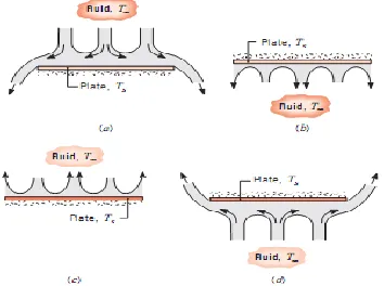
As from the figure 2.2.2

Upper Surface of Hot Plate or Lower Surface of Cold Plate:

𝑁𝑢𝐿 = 0.54 𝑅𝑎𝐿 1

4₍₁₀4_{≤ 𝑅𝑎}

𝐿 ≤ 107, Pr ≥ 0.7 )

𝑁𝑢𝐿 = 0.15 𝑅𝑎𝐿 1

3₍₁₀7_{≤ 𝑅𝑎}

𝐿 ≤ 1011, 𝑎𝑙𝑙 𝑃𝑟 )

Lower Surface of Hot Plate or Upper Surface of Cold Plate:

𝑁𝑢𝐿 = 0.52 𝑅𝑎𝐿 1

5₍₁₀4_{≤ 𝑅𝑎}

(9)

Fig. 2.2.2 Buoyancy- driven flows on horizontal cold () and hot () plates : (a) Top surface of cold plate. (b) Bottom surface of cild plate. (c) Top surface of hot plate. (d) Bottom surface of hot plate.

III.EXPERIMENTAL SET UP

3.1 Materials Requirement

The materials required for the experimental set up are collected. They are given as follows:- 1) Wooden block

2) Metal plates 3) Thermocol 4) Thermocouple 5) Heating element and 6) Plyboard

Their main characteristics can be given as follows:-

1. Wooden Block:

It is the base of the set up. Upon which the heating element, metals plates, thermocouples etc are mounted on. It prevents heat losses from the metal plates because of its insulation properties.

2. Metal Plate:

Two iron plates of size 12.6𝑐𝑚 × 78𝑐𝑚 are used.

A metal plate is mounted on the wooden block and heating elements are place above the metal plate, which is then cover by the other metal plate. The thermocouples are fixed in zigzag pattern. It is heated with the help of heating element and its temperature difference is measured.

3. Thermocol:

(10)

4. Thermocouple:

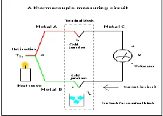
A thermocouple is a device used extensively for measurement of the temperature of the body. It is a device made by two wires of different metals joined at one end, called Junction end or measuring end. The two wires are called thermoelements or legs of the thermocouple: the thermoelements are distinguished as positive and negative ones. The other end of the thermocouple is called is tail end or reference end. It is shown as in fig.

Fig. 3.1.4 Thermocuople measuring circuit

Working Principle:-

The working principle of thermocouple is based on three effects, discovered by Seebeck, Peltier and Thomson. They are as follows:

A. Seebeck Effect:

The seebeck effect states that when two different or unlike metals are joined together at two junctions, an electromotive force (emf) is generated at the two junctions. The amount of emf generated is different for different combinations of the metals.

This relationship is expressed by the Seebeck coefficient, ∝𝐴𝐵defined as

Fig. 3.1.4(a) Seebeck Effect

B. Peltier Effect:

As per the Peltier effect, when two dissimilar metals are joined together to form two junctions, emf is generated within the circuit due to the different temperatures of the two junctions of the circuit. The Peltier is proportional to the current flowing through the junction; the proportionality constant is the Peltier coefficient 𝜋𝐴𝐵 and the heat transfer required to maintain a

constant temperature is 𝑄𝐴𝐵= 𝜋𝐴𝐵𝐼

(11)

Fig.3.1.4(b) Peltier Effect

C. Thomson Effect:

As per Thomson effect, when two unlike metals are joined together forming two junctions, the potential exists within the circuit due to temperature gradient along the entire length of the conductors within the circuit.

The emf suggested by the Thomson is very small and can be neglected.

𝑄𝜍 = 𝜍. 𝐼( 𝑇2− 𝑇1 )

Where 𝜍 is the Thomson coefficient.

Fig.3.1.4(c) Thomson Effect

5. Heating Element:

The heating elements are placed in between the wooden block and metal plate. They consist of metal plates of small dimension. They are heated with the help of power supply.

6. Ply-Board:

Two plyboards are used as side guard in the set up on either side of the model.

The main purpose of plyboard is to prevent heat losses from the heating element and also to maintain uniform flow of air over the metal plate.

3.2 Steps of Construction:-

The required steps of construction are given as follows:-

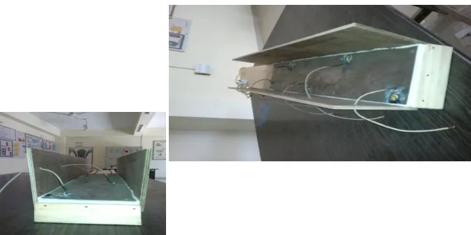
1. First, the metal plate is placed on the wooden block and then the heating elements are fixed above the metal plate, where the other metal plate is again placed on the whole set up which is fixed by nuts.

2. The thermocol is placed between the two metal plates, which help to heat stop the heat escape between the two metal plates as it acts as an insulator. These heating elements are connected to power supply.

3. The thermocouples are fixed on the front side of the second metal plate in zig-zag manner at regular interval. The number of readings to be taken is depended upon the number of thermocouples fixed on the metal plate.

4. As five thermocouples are fixed at different distances, in the model. Five different readings are taken.

(12)

6. A reference thermocouple is soldered on the metal plate. This acts as the reference point for the whole experimental set up.

Fig 3.2.1 Working Model

3.3 Working of The Model:-

When supply power, the metal plates get heated with the help of heating element. The air above the metal plate is also heated due to heat transfer through convection. The temperature of the air above the metal plate gradually increases and a stage will come when the temperature of the air will remain constant. The change in temperature of the metal plate is measured with the help of thermocouples placed at regular intervals and at different distance from the initial point. The thermocouple is connected to a galvanometer for measuring the emf arises due to change in temperature.

Thus, the heat transfer rate over a flat plate due to convection is calculated at different distances from the reference point.

3.4 Method of Experiment

The mechanism of heat transfer in which fluid motion produced due to change in density resulting from temperature gradient is known as natural convection. The fluid particles in the immediate vicinity of the heated surface become warmer than surrounding fluid resulting in a local change of density. The warmer fluid is replaced by the colder fluid and that upward movement of warmer particles and downward movement of cold particles is called convection currents. The force which includes these convections is called buoyancy force which is due to presence of a density gradient within the fluid and body force. Equations are derived by boundary layer through various empirical and semi empirical co-relations for free convections valid for different configurations and conditions are available.

(13)

h= f (d, ρ, µ, g, Cp, K, ß, θ)

Solving the equation by the Buckingham’s π theorem, we get 𝑕×𝑑

𝐾 = A (µ×Cp / K) (d³×ρ²× ß × g × θ/ µ²)

Where, 𝑕×𝑑

𝐾 = Nusselt number = Nu

𝜇 ×𝐶𝑝

𝐾 = Prandalt number = Pr

𝑑

3_×𝜌2_{×𝛽 ×𝑔×𝜃}

𝐾 = Grashoff number = Gr

EMPIRICAL RELATION

For free convection heat flow over vertical plate the local heat transfer coefficient in laminar flow is given by Nu = 0.48 ( Gr ) ¼ (Pr )½ (0.861+Pr)‾¼

The properties of fluid are calculated at mean temperature of the plate surface and fluid in laminar flow and average heat transfer coefficient relation is given by

104 < Gr×Pr < 107 Nu = 0.56 (Gr×Pr) 1/4

In turbulent flow average and local heat transfer coefficient is given by 108 < Gr×Pr < 1012

Nu = 0.13 (Gr×Pr)1/3

PROCEDURE

Variac is set to the required position and vertical copper plate is heated by means of heater. Wait for an hour to establish steady state condition and then note down the readings of temperature at equidistance of 7.8 cm on the plate and also note down air temperature.

(14)

CALCULATIONS

To find out local heat transfer coefficient at 0.078m distance from base of the plate (h0.078):

Step 1, Tm = tx + ta

2 & tx = temp. at 0.078m on the plate

Where, β = 1/ Tm

For properties of air at tm ˚C, find υ, k, Pr

Step 2,

Grx =

𝛽 ∗𝑔∗𝑥3 ( 𝑡𝑥 – 𝑡𝑎 )

𝑢2 where x = 0.078m

Now, Ra = Grx * Prx

For, 105 < Ra < 108 C = 0.56 & n = 1/4 Step 3,

Grx * Prx =

Hence, Nux = C (Ra) n

Also, Nux =

𝑕0.078 ∗ 𝑋 𝑘

Find, h0.078 =

Making same calculations for other readings, find values of h0.156, h0.234, h0.312… Average heat transfer coefficient

Take the total mean of the whole temperature reading we get, tsav =

𝑡𝑥 1 + 𝑡𝑥 2 + 𝑡𝑥 3 +⋯+ 𝑡𝑥 10 10

From there we get, Tm = 𝑡𝑠𝑎𝑣 + 𝑡𝑎

2 & β = 1/ Tm

From properties of air at tm ˚C, find υ, k, Pr

Now, Gr = 𝛽 ∗𝑔∗𝑙3 ( 𝑡𝑠𝑎𝑣 – 𝑡𝑎 )

𝑢2 where, l = length of the plate = 0.078m

Gr * Pr = __

Nu = C ( Gr *Pr ) n Also, Nu = 𝑕𝑎𝑣 ∗𝐼

𝑘

Now we will find, hav =

(15)

IV.RESULTS AND DISCUSSION

RESULT TABLE

DISCUSSION

As from the observation and the result table, it is shown that the temperature at different point form the base varies under laminar and steady flow condition, The longer the plate is heated, under constant (same amount) supply of power, it will increase the temperature but under the steady flow condition and the average heat transfer coefficient will not change at different points.

The variation in the heat transfer are due to unsymmetrical placing of the heater and the Gr no keep on increasing corresponding to the buoyancy i.e. Gr increases when buoyancy increases.

V.CONCLUSION

From this experiment, it can be found out local and average heat transfer coefficient of a vertical flat plate. The average heat transfer coefficient is 6.0287 W/𝑚2_{. K}

Scope of Future Work

The present computation and experiment has been carried out for heat transfer by natural/free convection over a flat plate. It can be further extended for forced convection using fan and blower or mixed convection can also be performed. It can be further extended by inclining the plate by different angles and taking the heat transfer rate at different angles and comparing them and making analysis on that.

(16)

REFERENCES

1. Introduction to Heat Transfer 6th_{edition by Theodore l. Bergman/ Adrienne s. lavine/ Frank p. incropera/David p. Dewitt} 2. Heat Transfer 2nd Ed., By Yunus A. Cengel

3. Laljee R.P., Muddaiah S., Salagundi B., Cariappa P.M., Indra A.S., Sanjay V., Ramanathan A., "Interferon stimulated gene - ISG15 is a potential diagnostic biomarker in oral squamous cell carcinomas", Asian Pacific Journal of Cancer Prevention, ISSN : 1513-7368, 14(2) (2013) pp.1147-1150. 4. Heat and mass Transfer, By D.S. Kumar

5. Kumar S., Das M.P., Jeyanthi Rebecca L., Sharmila S., "Isolation and identification of LDPE degrading fungi from municipal solid waste", Journal of Chemical and Pharmaceutical Research, ISSN : 0975 – 7384 5(3) (2013) pp.78-81.

6. Analysis of Forced Convection Heat Transfer over a Flat Plate Using MATLAB Graphical User Interface, M.M. Rahman, Z.M. Hasib, and Dr. M. A. Rashid Sarkar , 8th Control Instrumentation and System Conference (CISCON-11) – An International Conference.

7. Sundar Raj M., Arkin V.H., Adalarasu, Jagannath M., "Nanocomposites based on polymer and hydroxyapatite for drug delivery application", Indian Journal of Science and Technology, ISSN : 0974-6846, 6(S5) (2013) pp.4653-4658.

8. 8. Rajesh Khatri, Pankaj Agrawal2_{, Mohan Gupta}3_{, Jitendra verma}4_{, 1-4Department of Mechanical Engineering, Samrat Ashok Technological} Institute, Vidisha (M.P) 464001, India. 2 Professors in Department of Mechanical Engineering, Samrat Ashok Technological Institute, Vidisha (M.P.) 464001, India. 3 Department of Mechanical Engineering, R.K.D.F, Bhopal, (M.P) 462003, India. Laminar flow analysis over a flat plate by computation fluid dynamics, International journal of advances in Engineering and Technology, may 2012.

9. Vijayaprakash S., Langeswaran K., Gowtham Kumar S., Revathy R., Balasubramanian M.P., "Nephro-protective significance of kaempferol on mercuric chloride induced toxicity in Wistar albino rats", Biomedicine and Aging Pathology, ISSN : 2210-5220, 3(3) (2013) pp.119-124.

10. Some solution for external laminar forced convection, me.queensu.ca/Courses/831/files/CONVBK03_Secure.pdf.

11. Sundararajan M., "Optical instrument for correlative analysis of human ECG and breathing signal", International Journal of Biomedical Engineering and Technology, ISSN : 0976 - 2965, 6(4) (2011) pp.350-362.

12. P Thamarai, B Karthik, Automatic Braking and Evasive Steering for Active Pedestrian Safety, Middle-East Journal of Scientific Research 20 (10), PP 1271-1276, 2014.

13. M.Bharathi, Golden Kumar,Design Approach For Pitch Axis Stabilization of 3-Dof Helicopter System an LQR Controller,International Journal of Advanced Research in Electrical, Electronics and Instrumentation Engineering,ISSN 2278 - 8875 , pp 351-365 ,Vol. 1, Issue 5, November 2012. 14. SRIDHAR RAJA. D ,Foliated UC-EBG UWB Bandpass filter ,International Journal of Advanced Research in Electrical, Electronics and

Instrumentation Engineering ,ISSN (Print) : 2320 – 3765,pp 3701-3708,Vol. 2, Issue 8, August 2013.

15. V.M. Ramaa Priyaa,Predictive Control in Power Converters,International Journal of Advanced Research in Electrical, Electronics and Instrumentation Engineering, ISSN (Print) : 2320 – 3765 , pp 10475-10478 ,Vol. 3, Issue 7, July 2014.

16. Vijayan T ,Performance of Microstrip Directional Coupler Using Synthesis Technique,International Journal of Advanced Research in Electrical, Electronics and Instrumentation Engineering, ISSN: 2278 – 8875, pp 761-767,Vol. 2, Issue 3, March 2013.

17. Vijayan T ,Performance Image Compression using Lifting based EEWITA,International Journal of Advanced Research in Electrical, Electronics and Instrumentation Engineering,ISSN (Print) : 2320 – 3765, pp 10501-10508,Vol. 3, Issue 7, July 2014.

18. Model6, http://www.scribd.com/doc/104900241/24342700-Student-Slides-M6

ANNEXURE 1

With the calculation of the available data from the experiment reading, it has been found that the total mean temperature is 42.32ᵒC (Tm). Where the volumetric expansion coefficient (β = 1/ Tm) is and Grashof (Gr) no. is 4.72*108_{and the value of average heat}

transfer (𝑕𝑎𝑣) calculation are carried out from the given formula,

Nu = 𝑕𝑎𝑣 ∗𝐼

𝑘

Where the average heat transfer (𝑕𝑎𝑣) = 6.0287 W/𝑚2_{. K}

Practical average heat transfer coefficient q = h.A. T

(17)

∆𝑇 = 47.84 − 36.8 = 11.04 ℃ q = 46 watt

h = 46

0.10062 ×11.o4 = 41.41 W/m

2 .K

Constant value

Kinematic viscosity, 𝑣 = 16.47 N.s/m2 Prandlt number, Pr= 0.711

Thermal conductivity, k = 0.0271 W/m. K

CALCULATION

𝑇𝑚1 = 43.35

𝛽1 = 0.00316𝑘−1

𝑋1 = 0.078m

𝐺𝑟𝑥1 =

0.003×9.81×(49.9−36.8)(0.078)3

(16.47×10−6₎2

=4.46× 106

𝑕𝑥1 = 𝐾×𝑁𝑢𝑥 1

𝑥 , where K=0.0271

=23.629×0.0271

0.078

=8.209 W/𝑚2_{. K}

Average heat transfer coefficient, 𝑇𝑠𝑎𝑣 = 47.84

𝑇𝑚 = 𝑇𝑠𝑎𝑣 + 𝑇𝑎

2

=47.84 + 36.8 = 42.32ᵒ𝐶

Gr = 𝛽 ×𝑔 ×𝑙3(𝑇𝑠𝑎𝑣 − 𝑇𝑎 )

𝑢2

=0.00315 ×9.81 × 0.78 3(47.8−36.8)

(16.47 ×10−6₎2

= 6.379 × 108

Pr = 0.711

Gr × 𝑃𝑟 = 4.72 × 108

C = 0.13, n =1

3 = 0.33

Nu = 0.13(4.72 × 108₎.33

= 90.544 𝑕𝑎𝑣 = 𝑁𝑢 ×𝐾

𝑙

=90.544 ×0.0271

0.78