Statistical Estimation of Crack Growth Behaviors in Steam Generator Tubes Using Monte Carlo Method

(1)

18th International Conference on Structural Mechanics in Reactor Technology (SMiRT 18) Beijing, China, August 7-12, 2005 SMiRT18-M02-6

STATISTICAL ESTIMATION OF CRACK GROWTH BEHAVIORS IN

STEAM GENERATOR TUBES USING MONTE CARLO METHOD

Jae Bong Lee

Chungbuk National University, Cheongju,

Chungbuk, 361-763, Korea

Phone: 82-043-264-2460

E-mail: leejb@chungbuk.ac.kr

Jai Hak Park

Chungbuk National University, Cheongju,

Chungbuk, 361-763, Korea

Phone: 82-043-264-2460

E-mail: jhpark@chungbuk.ac.kr

Sung Ho Lee, Hong-Deok Kim, Han-Sub Chung

Korea Electric Power Research Institute, Yusonggu, Daejun, 305-380, Korea

ABSTRACT

The growth of stress corrosion cracks in steam generator tubes is estimated using the Monte Carlo simulation and statistical approaches. The statistical parameters that represent the characteristics of crack growth and crack initiation are derived from in-service inspection (ISI) NDE data. Based on the statistical approaches, crack growth models are proposed and applied to estimate crack distribution at the end of cycle (EOC). Because in-service inspection (ISI) crack data is different from physical crack data, a simple method for predicting the physical number of cracks from periodic in-service inspection data is proposed in this study. Actual number of cracks is easily estimated using the method, and the statistical crack growth is simulated using the Monte Carlo method. Probabilistic distributions of the number of cracks and maximum crack size at EOC are obtained from the simulation. Comparing the predicted EOC crack data with the known EOC data the usefulness of the proposed method is examined and satisfactory results are obtained.

Keywords: Statistical Assessment, Integrity, Monte Carlo Method, Steam Generator Tube

1. INTRODUCTION

Statistical approaches are widely used for assessment of structural integrity in power industries. One approach is the probabilistic fracture mechanics approach, in which probabilistic contents are introduced into deterministic fracture mechanics theory (Maeda, et al., 2002). This method is useful for analyzing local problems. But it has difficulties in treating large structures because of a lot of variables (load, material properties, crack size, and position etc.) and its complex theory.

(2)

In order to calculate the probability of failure or to estimate the amount of leakage, it is necessary to know the number of physical flaws and their size distribution. Here the physical cracks are defined as the cracks that are expected to exist actually in steam generator tubes. But in-service inspection (ISI) crack data is different from the physical crack data, because inspection systems have imperfection in detecting cracks and measuring their sizes. For estimating the physical number of cracks from periodic in-service inspection data a simple method is proposed.

The statistical crack growth is simulated using the Monte Carlo method in order to estimate the number of cracks and the maximum size distribution at interesting time. The necessary statistical characteristics for crack growth rate and crack initiation are calculated from real NDE data.

2. MODELS FOR CRACK GROWTH ESTIMATION

BOC crack (ith_cycle)

EOC crack (ith_cycle)

NDE crack (i-1th_ISI)

Size & detection uncertainty Repaired tubes

Crack initiation

- from Weibull function.

- Probabilistic crack growth rate

Detected crack growth

Undetected crack growth

- Determine crack size

- Probabilistic crack growth rate

BOC crack (ith_cycle)

EOC crack (ith_cycle)

NDE crack (i-1th_ISI)

Size & detection uncertainty Repaired tubes

Undetected crack growth

- Probabilistic crack growth rate Undetected crack growth

- Probabilistic crack growth rate

Fig. 1 Procedure of statistical analysis model for crack growth.

Fig. 1 illustrates the procedure used in the proposed statistical model for crack growth estimation. The model estimates the number of cracks and their size distribution at the end of ith cycle using the NDE data at (i-1)th ISI. Calculation process of crack growth is subdivided into crack initiation, undetected crack growth and detected crack growth. For the calculation, the information on the crack initiation and the crack growth rate are necessary and the number of physical cracks also must be known. The statistical characteristics of crack initiation and crack growth rate are represented with statistical distribution functions whose parameters are obtained from statistical analyses of ISI NDE data. It is necessary to know the number of physical flaws and their size distribution in order to calculate the probability of failure or to estimate the amount of leakage through the tube wall of steam generators. Therefore the initiated cracks in ith ISI and their size distributions are estimated in physical domain.

(3)

3. CALCULATION OF CRACK GROWTH RATE

The crack growth rate used in the simulation is statistically calculated from the in-service non-destructive inspection data. Fig. 2 shows crack growth rate data in tubes of model F steam generators (SG) in Korea. The model F steam generators have been operated for 12.38 EFPY (effective full power year) and 12 in-service inspections were made. The crack growth rate at ith inspection is obtained by dividing the crack length increment by the time interval between ith and (i+1)th inspections. The units of crack length and time are mm and EFPY respectively. Many data points in Fig. 2 show negative crack growth rates, which are inconsistent values. The negative growth rate is due to the uncertainty of NDE.

0 1 2 3 4 5 6 7

-3 -2 -1 0 1 2 3 4 5

Cr

ack Growt

h

Rate

(m

m

/EFPY)

Crack length(mm)

Fig. 2 NDE crack growth rate data (model F SG).

4 5 6 7 8 9 10 11 12 13

2 3 4 5 6 7 8

Cr

ack lengt

h(mm)

ISI

NDE crack length data regression curve using

1st or 2nd order polynomial

Fig. 3 Regression of crack length data with polynomials.

Fig. 3 shows the crack length data measured at each ISI. It can be noted that the crack length does not increase always. In order to obtain nonnegative and more consistent crack growth rate values, the regression analysis is done for the crack length data at each ISI using a polynomial. Several results of the regression analysis are given in Fig. 5. When the number of data points is less than 4, the linear regression is used. However when the number of data points is equal to or more than 4, the polynomial of the second degree is used for the regression. The crack growth rate is the gradient of the regression curve at the time.

(4)

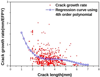
that the crack growth rate decreases as the crack length increases. This result is consistent with the previous studies (Chung, 2000).

0 1 2 3 4 5 6 7 8

0 1 2 3

Crack growth rate Regression curve using

4th order polynomial

Cra

ck gr

owt

h

ra

te(

m

/E

F

PY

)

Fig. 4 Crack growth rate data and regression with a polynomial

.

1 1

0.01 0.1 1 10

0 Crack growth rate

Regression curve in Figure 5

(4th order polynomial)

y=Caγ regression curve

Crac

k g

ro

w

th

ra

te(

mm

/EF

PY

)

Fig. 5 The regression analysis of crack growth rate.

The crack growth rate is assumed to satisfy the following equation (Wu, 1995):

z

a

f

dt

da

)

(

=

(1)

where a is crack length, t is time and f(a) is a function of the crack length a. And z is a statistical random variable and used to represent random error. One simple form of Eq. (1) is the following:

z

Ca

dt

da

₌

λ

(2)

where C and λ are constants. Taking logarithm to both sides of Eq. (2) leads to:

z

log

a

log

C

log

dt

da

log



=

+











_λ

(3)

(5)

polynomial is also plotted. It can be noted that the difference between the linear regression line and the fourth order polynomial is small.

And log z is obtained by statistical analysis of error term. Based on linear regression theory (Mendenhall, 2003), the term, log z in Eq. (3) can be statistically described with the sum of squares for error (SSE) or standard error of estimate (root mean of squares for error, RMSE), which is calculated from:

2

−

=

−

=

∑

n

SSE

n

)

Yˆ

Y

(

RMSE

i (4)

Where Yi is crack growth rate data, Yˆ is the value calculated from regression equation and n is the number of

data points. Therefore log z is expressed by normal distribution, N(0, RMSE2) and we can obtain statistical crack growth rate using Eq. (3).

4. UNCERTAINTY OF DETECTION AND THE NUMBER OF PHYSICAL CRACKS 4.1 Probability Of Detection

Non-destructive inspection systems have been operated in their extreme capability for finding small cracks. In fact, the cracks of the same size may give different inspection results and it is called the uncertainty or imperfection of NDE systems.

The uncertainty of NDE is subdivided into the uncertainty of size and the uncertainty detection. The uncertainty of size is often characterized in the simplest form of a statistical model of a linear or linearized regression to the measured versus true size data. The uncertainty of detection is characterized in terms of the probability of detection (POD) and given as a function of crack size. The uncertainty of size is not difficult to handle but the POD is sophisticated and complicated.

At present, the POD can be estimated only through inspection reliability experiments on specimens containing flaws of known size. Further, statistical methods are used for quantifying the experimental error in the estimating capability.

The POD is usually represented by the log-logistics (log odds) function or practically equivalent cumulative log normal distribution function. Eq. (5) and Eq. (6) represent the cumulative log-logistics function and the log normal function respectively (Berens, 1989)and Fig. 6 represents general shape of POD curve.

(

)

(

a

)

a a ln exp 1 ln exp ) ( POD 1 0 1 0 β β β β + − +

= (5)

1 3 1 POD −                   − − + = σ µ π lna exp

) a

( (6)

In Eqs. (5) and (6), β0, β1, µ and σ are the parameters of these functions and can be estimated using the maximum likelihood analysis (Berens, 1989). These parameters are related by:

1 0

β

µ

=− (7)

) 3 (

β

₁

π

(6)

0 5 0.0

0.2 0.4 0.6 0.8

1.0 POD(a) curve

POD

(Pr

oba

bi

lity

o

f de

te

c

ti

on)

Flaw size

Fig. 6 General shape of POD(a) curve

4.2 Calculation of Physical Cracks

It is easy to obtain the physical sizes from the NDE crack size data once the size uncertainty of the inspection method is known. And in case of a single inspection, it is also easy to estimate the number of physical number of cracks using the POD curve. However, we may be faced with some difficult problems in obtaining the physical number of cracks from the periodic in-service non-destructive inspection data. Cracks can be detected after they reach the minimum detectable crack size. Some cracks are detected immediately after reaching the size, while some cracks are detected after several inspections. In order to calculate the number of physical cracks, the inspection history of each crack must be known. But it is nearly impossible to know the individual inspection history, so an estimation procedure is necessary. As a previous work, Davis (2001) has estimated the physical crack distribution from the measured initial crack distribution using POD without consideration of repeated inspections. The physical crack is defined as the estimated crack, which physically exists in tubes including undetected cracks. Because the capability of NDE system is not perfect, we can easily assume that other cracks exist besides detected NDE cracks. The method of calculating the number of physical cracks is easily derived from the definition of POD.

flaws physical of

number The

s flaw detected of

number The

a

POD( )=

(9)

) (a POD

number The

number

The =

(10)

In Eq. (9), POD means that how many cracks could be detected among physical cracks, which actually exist in SG tubes and it depends on crack size. The number of physical cracks is easily calculated by Eq. (10) theoretically (Davis, 2001). But Eq. (10) cannot be applied to periodic ISI NDE data, because the equation does not consider repeated NDE inspections at each end of cycle (EOC). In the case of periodic inspection, more sophisticated method need to be used for calculating the number of physical cracks.

In order to calculate the number of physical cracks with periodic NDE data, both probabilities of detecting and missing cracks should be considered. The probability of detecting a crack through n times of inspections is calculated using the probability of missing the crack.

(7)

(

)

x n x

q

p

x

n

x

n

q

p

x

n

₋ ₋

−













!

=

(11)

Here p is the POD and q (=1− p) is the probability of miss. And the probability of detecting a crack at least once through n times of inspections becomes:

(12)

(

)

n

p

P

=

1 −

But we confront essential problems in applying Eq. (12) to real periodic ISI data. In order to calculate the probability of detection through n times of inspections, we have to know the exact crack growth history and the number of inspections for each crack. But it is nearly impossible to know them.

For periodic inspections, the probability of detection is different from POD because each crack can be examined more than once. Let the total probability of detection be “effective POD”. Then the number of physical cracks is expressed as the following:

OD(a) effectiveP

number The

number

The =

(13)

And in order to know the crack growth history and the number of inspections for each crack, a statistical simulation approach is used.

4.3 Simulation for Effective Probability of Detection

Fig. 7 Schematic diagram of a statistical simulation for estimating crack growth history.

Fig. 7 shows the statistical simulation schematically. Let a crack with 2.7mm length be detected at ith ISI for the first time. Using the backward crack growth simulation, the crack size history can be obtained. Since POD is a function of crack size, the POD values also can be calculated at each ISI. From the obtained POD values the total POD, i.e. the effective POD can be calculated. By repeating the simulation many times, the mean value of the effective POD is obtained.

For the given inspection system, the effective POD is obtained as a function of crack size at each ISI. The number of physical cracks for the given length or length interval is obtained from Eq. (13).

The effective POD curve at each ISI is obtained using the following procedure. The backward flaw growth simulation is made using the Monte Carlo method. The effective POD curve at k-th ISI is obtained as follows;

(8)

(2) Do the Backward crack growth simulation until the crack length becomes shorter than the minimum detectable crack length. During the simulation a random variable z is generated and the crack growth rate is obtained from Eq. (2).

(3) Obtain the crack sizes and the corresponding POD values at each previous ISI. (4) Calculate PODEff from the obtained POD values.

(5) Generate many PODEff values by repeating the steps from (1) to (4), and calculate the mean value of PODEff.

(6) Repeat the steps from (1) to (5) for a crack with the increased length ai+∆a at k-th ISI to obtain the mean value of PODEff for different crack size.

Table 1 POD values for each crack length range at each ISI.

size

IS I 0.5~ 1.5 1.5~ 2.5 2.5~ 3.5 3.5<

4 ~ 9 0 0.4 0.8 1

10 ~ 12 0.4 0.8 1 1

PO D

The POD value used in the simulation is represented in Table 1. In the simulation, discrete POD values are used, because it is more convenient to count the number of flaws and calculate the number of physical flaws.

0 1 2 3 4 5

0.0 0.2 0.4 0.6 0.8 1.0

POD curve 1 ~ 9 ISI 10 ~ 12 ISI

POD (Pro

bab

ility

of

Dete

cti

on)

Figure 8. Continuous and discrete POD curves.

Fig. 8 show the discrete and continuous POD curves used in the simulation at each ISI. Since NDE system has been changed after 9th ISI, the POD curve is also changed after 9th ISI.

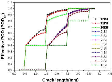
0.0 0.5 1.0 1.5 2.0 2.5 3.0 3.5 4.0 4.5 0.0

0.1 0.2 0.3 0.4 0.5 0.6 0.7 0.8 0.9 1.0 1.1

E

ffecti

ve POD

(P

OD

Eff

)

12ISI 11ISI 10ISI

9ISI 8ISI 7ISI 6ISI 5ISI 4ISI 3ISI 2ISI 1ISI

Figure 9. POD

Eff

curves obtained from the simulation.

(9)

As repeating the inspection, PODEff values become lager and show large disparity comparing with the initial POD value. And we can find that PODEff curve reflects the effect of the change of NDE system at the 10th ISI.

PODEff is applied for estimating the number of physical flaws from NDE data. Fig. 10 shows the comparison of each estimated number of physical flaws using POD and PODEff by Eq. (10) or (13).

3 4 5 6 7 8 9

0 100 200 300 400 500 600 700 800

Physical (POD) Physical (POD

Eff)

NDE data

T

h

e

number of c

ra

c

k

e

d

tube

s

EFPY

Figure 10. Number of physical cracks obtained using POD and POD

Eff

.

The estimated number of physical flaws using POD is lager than that obtained using PODEff. So conservative estimation is possible when POD is used instead of PODEff.

Because we don’t know the exact number of physical flaws without the destructive experiment, we cannot determine which method is more accurate. Because the logic of simulation for PODEff is reasonable, the estimated number of physical flaws using PODEff may be more similar with real one.

4.4 Crack Initiation

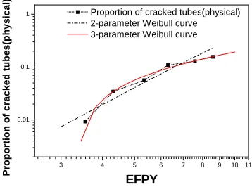
The number of initiated cracks during ith operation cycle is predicted from statistical analysis of NDE data obtained until (i-1)th ISI. Using the Weibull distribution function, the number of initiated cracks at ith ISI is predicted. Fig. 11 illustrates cumulative proportion of initiated cracks at each ISI and their fitting curves with 2-parameter and 3-parameter Weibull distribution functions. The cumulative proportion of initiated cracks is calculated in physical domain, i.e. the number of initiated physical cracks is calculated. It is noted that the 3-parameter Weibull curve is more coincident with data points than the 2-parameter Weibull curve as shown in Fig. 11. Therefore the 3- parameter Weibull function is used for estimating the number of initiated cracks in the simulation.

3 4 5 6 7 8 9 10 11

0.01 0.1

1 Proportion of cracked tubes(physical)

2-parameter Weibull curve 3-parameter Weibull curve

P

rop

ort

ion

o

f cr

acked

tub

e

s(p

h

ysi

cal)

EFPY

(10)

5. SIMULATION RESULTS

The number of cracks and their sizes are predicted statistically using the Monte-Carlo simulation represented in Fig. 1. Using NDE data of model F steam generators at the 8th ISI, the number of initiated cracks and maximum crack size at the 9th ISI are predicted. The simulation is repeated 1000 times and results are statistically analyzed, thereby the results are obtained as probabilistic distributions.

Predicted numbers of newly initiated physical cracks during the 9th operation cycle are given in Table 2 for 50%, 90% and 95% confidence levels. The prediction is made using the 3-parameter Weibull function as explained in the section 4.4. The value corresponding to 50% confidence level shows similar crack numbers to 88 cracks, which is the number of physically initiated cracks calculated from NDE data at the 9th ISI.

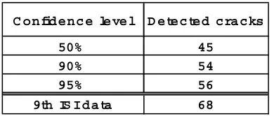
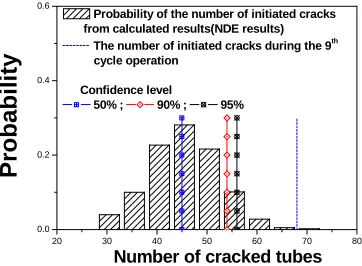
It is also necessary to predict the number of newly detected cracks as well as the number of physical cracks. Fig. 12 illustrates the probabilistic distribution of the number of newly detected cracks at the 9th ISI. And the values corresponding to 50%, 90% and 95% confidence levels are also given in Fig. 12 and Table 3. Comparing with the NDE data of 68 cracks at the 9th ISI, simulation results show somewhat smaller crack numbers. The reason of this underestimation may be that the used POD is larger than the true POD.

Even if there is discrepancy between the predicted number of cracks and the NDE data it is limited to the cracks with short length. For the long cracks, the predicted number of detected cracks is always nearly the same as the number of NDE cracks because the POD and the effective POD have the values close to 1.

Table 2 Estimated numbers of newly initiated physical cracks during the 9

th

cycle operation

for several confidence levels

C o n fid e n c e le ve l N e w ly in itia te d

p h ys ic a l c ra c ks

50% 95

90% 109

95% 112

9th IS I d a ta 88

Table 3 Estimated numbers of newly detected cracks at the 9

th

ISI for several confidence

levels

C o n fid e n c e le ve l D e te c te d c ra c ks

50% 45

90% 54

95% 56

(11)

20 30 40 50 60 70 80 0.0

0.2 0.4 0.6

Probabil

it

y

Number of cracked tubes

Probability of the number of initiated cracks

from calculated results(NDE results)

The number of initiated cracks during the 9th

cycle operation

Confidence level

50% ; 90% ; 95%

Fig. 12 Probabilistic distribution of the estimated number of newly detected cracks at the

9

th

ISI from the simulation.

Fig. 13 illustrates probability density distributions of crack size corresponding to the 50th, 90th and 95th percentiles at the 9th ISI. The distributions are obtained from 1000 simulation results. The distribution for the maximum crack size also can be obtained, but unusually large maximum crack sizes are often observed. That is due to the probabilistic crack growth rate and the large random error, z in Eq. (3). Therefore we can get more consistent estimated value for the maximum crack size if we use the percentiles instead of the maximum crack size distribution. The percentiles for crack size corresponding to three confidence levels are given in Table 4. The maximum crack size measured at the 9th ISI is 6.8mm and the 99% percentile crack size corresponding to 50% confidence level shows the most similar value.

Table 4 The 50

th

, 90

th

, 95

th

and 99

th

percentiles for crack size with 50%, 90% and 99%

confidence level from simulation results.

C o nfidence

level 50

th

90th 95th 99th

50% 3.2 5.4 6.6

90% 3.3 5 5.5 7

99% 3.3 5.1 5.6 7.6

9th IS I M ax. 6.8 6.8 6.8 6.8

The xth percentile for crack size

4.9

2.5 3.0 3.5 4.0 4.5 5.0 5.5 6.0 6.5 7.0 7.5 8.0 8.5 9.0 0

2 4 6 8 10 12 14

P

robabil

it

y densit

y

Crack size (mm)

The probability density of xth percentiles

for crack size from simulation results

50th 90th 99th

The maximum crack size in the 9th ISI

(12)

6. CONCLUSION

The growth of stress corrosion cracks in steam generator tubes is estimated using the Monte Carlo method and statistical approaches. The statistical parameters that represent the characteristics of the crack growth and the crack initiation are derived from the In-Service Inspection (ISI) NDE data.

The proposed analysis method is applied to predict the crack distribution at EOC. Comparing the predicted EOC crack data with the known EOC data the usefulness of the proposed method is examined.

ACKNOWLEGEMENT

The authors are grateful for the partial support provided by a grant from the Korea Science and Engineering Foundation (KOSEF) and Safety and Structural Integrity Research Center at the Sung Kyun Kwan University.

REFERENCES

[1] Maeda, N., Nakagawa, S., Yagawa, G., and Yoshimura, S. (2002): “Optimization of operation and Maintenance of nuclear Power Plant by Probabilistic Fracture Mechanics”, Nuclear Engineering and Design, Vol. 214, pp. 1-12.

[2] ERPI NP-7493 (1991): “Statistical Analysis of Stream Generator Tube Degradation”.

[3] Chung, H.S., Kim, G.T., and Kim, H.D. (2000): “A Sturdy on the Integrity Assessment of Detected S/G Tube”, KERPI.

[4] Wu, W.F., and Syau, J.J. (1995): “A Study of Risk-Based Non-Destructive In-Service Inspection”, Nuclear Engineering and Design, Vol. 158, pp. 409-415.