Copyright2001 by the Genetics Society of America
Marker Pair Selection for Mapping Quantitative Trait Loci
Hans-Peter Piepho* and Hugh G. Gauch, Jr.
†*Institut fu¨r Nutzpflanzenkunde, Universita¨t Kassel, 37213 Witzenhausen, Germany and†Department of Plant Breeding, College of Agriculture and Life Sciences, Cornell University, Ithaca, New York 14583
Manuscript received January 27, 2000 Accepted for publication October 6, 2000
ABSTRACT
Mapping of quantitative trait loci (QTL) for backcross and F2populations may be set up as a multiple
linear regression problem, where marker types are the regressor variables. It has been shown previously that flanking markers absorb all information on isolated QTL. Therefore, selection of pairs of markers flanking QTL is useful as a direct approach to QTL detection. Alternatively, selected pairs of flanking markers can be used as cofactors in composite interval mapping (CIM). Overfitting is a serious problem, especially if the number of regressor variables is large. We suggest a procedure denoted as marker pair selection (MPS) that uses model selection criteria for multiple linear regression. Markers enter the model in pairs, which reduces the number of models to be considered, thus alleviating the problem of overfitting and increasing the chances of detecting QTL. MPS entails an exhaustive search per chromosome to maximize the chance of finding the best-fitting models. A simulation study is conducted to study the merits of different model selection criteria for MPS. On the basis of our results, we recommend the Schwarz Bayesian criterion (SBC) for use in practice.
P
ROCEDURES for detecting multiple quantitative problem of QTL detection and selection of cofactors isseen to be a single problem of finding the flanking trait loci (QTL) are of growing interest to plant
breeders and geneticists. The currently most widely used markers of QTL (LebretonandVisscher1998). This
puts us into the general framework of model selection
methods are interval mapping (IM; Lander and
Botstein1989, 1994) and composite interval mapping in multiple regression for which there is a vast
litera-ture (see,e.g.,Miller1990;DraperandSmith1998;
(CIM;Jansen1993;Zeng1993). In CIM, a chromosome
is scanned for the presence of a QTL, while controlling McQuarrieandTsai1998).
A peculiarity of multiple regression for QTL mapping for the genetic background using some markers as
cofac-is that there cofac-is no single true model, because there cofac-is
tors in a multiple regression framework (Zeng 1993;
no fixed set of markers. If we drop a pair of flanking
Jansen and Stam 1994). IM and CIM may be
imple-markers from the analysis, the dropped pair can be mented using the maximum-likelihood (ML) method
replaced by adjacent markers. Similarly, if a different
(Zeng 1994). Alternatively, an approximate
least-marker system is used, least-marker loci will change, but still
squares method can be used (HaleyandKnott1992;
the flanking markers will absorb the QTL effects,
lead-MartinezandCurnow1992;Whittakeret al.1996).
ing to a different model conditional on the markers. In this article we use the least-squares method.
Thus, the term “true model” has to be used with this
Whittakeret al.(1996) showed that the least-squares
peculiarity in mind.
method for IM and CIM in backcross (BC1) and F2
We believe that multiple LR testing (equivalently populations can be cast as a standard multiple linear
F-testing if linear least squares is used) for model selec-regression of phenotype on marker type, since
informa-tion is problematic for several reasons. Most impor-tion on the QTL is absorbed by the flanking markers
tantly, multiple likelihood-ratio (LR) tests without
ad-(Stam1991). Therefore, the problem of QTL detection
justments are known to tend to overfitting (Gelfand
essentially reduces to the problem of finding the
appro-andGhosh1998). For example, in multiple regression, priate pairs of markers. In CIM, we have the additional
using anF-to-enter statistic at the nominal␣ ⫽5% level task of selecting cofactors for controlling the genetic
in a forward selection procedure can easily give a true background. It may be argued that cofactors are useful
significance level (false positive rate) ⬎50% (Miller
for controlling genetic background only if they are
1990). Furthermore, only nested models can be com-closely linked to a QTL. In fact, the best control is
pared with LR tests. Also, the sequence of models to be expected for markers flanking the QTL. Thus, the dual
compared in a model-building process is not unique. One reaction to the problems connected with multi-ple LR testing is to consider a Bayesian framework (see,
Corresponding author:Hans-Peter Piepho, Institut fu¨ r
Nutzpflanzen-e.g.,Draper1995;Sillanpa¨a¨andArjas1998). A some-kunde, Universita¨t Kassel, Steinstrasse 19, 37213 Witzenhausen,
Ger-many. E-mail: [email protected] what intermediate approach, which is computationally
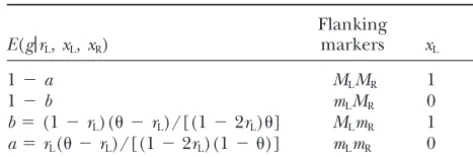
TABLE 1 much less demanding than many of the Bayesian
meth-ods, is to use information criteria such as Akaike’s infor- Expectation ofgconditional on flanking markers
mation criterion (AIC) or criteria assessing the mean for a BC1population
squared error of prediction such as Mallows’Cp(
Burn-hamandAnderson1998;GelfandandGhosh1998; Flanking
E(g|rL,xL,xR) markers xL xR
McQuarrie and Tsai 1998). Some selection criteria
such as theSchwarz(1978) Bayesian criterion (SBC) 1⫺a M
LMR 1 1
involve a Bayesian approach to model selection. A num- 1⫺b m
LMR 0 1
ber of different selection criteria are compared in the b⫽(1⫺rL)( ⫺rL)/[(1⫺2rL)] MLmR 1 0
a⫽rL( ⫺rL)/[(1⫺2rL)(1⫺ )] mLmR 0 0
present article.
Our suggested procedure is denoted as marker pair selection (MPS). Instead of implementing a standard
model selection procedure, we exploit knowledge of It can be shown, however, that E(g|rL, xL, xR) is linear in xL
andxR,i.e.,
the genetic mechanisms underlying the data. Our MPS procedure has three distinctive features: (i) markers are selected in adjacent pairs to increase the chance of
E(g|rL,xL,xR)⫽ ␣ ⫹ xL⫹ xR
selecting flanking markers while reducing the risk of
with
selecting nonflanking markers; (ii) an exhaustive search per chromosome is used in place of simple forward
⫽( ⫺rL)(1⫺ ⫺rL)
(1⫺ )(1⫺2rL)
and ⫽rL(1⫺rL)(1⫺2)
(1⫺ )(1⫺2rL)
selection, which increases the chance of finding the
best-fitting model; and (iii) a model selection criterion (4)
such as SBC is employed to select the final model among (compare to
Whittakeret al.1996; note that we use a slightly
a sequence of models. different coding here; the formula for a BC
1given in that
article is for a coding ofxLandxRas 1 and⫺1, not 0.5 and
⫺0.5 as erroneously stated in the article;John Whittaker, personal communication). Defining0⫽ ␥ ⫹a␣, L⫽ ␣,
MATERIALS AND METHODS
andR⫽ ␣, the expectation forYj, conditional on the mark-In this section, we describe the model for mapping QTL ers, can be written
in a backcross population as well as the method for parameter
E(Yj|rL,xL,xR)⫽ 0⫹ LxL⫹ RxR. (5)
estimation. We then develop an MPS algorithm on the basis
of a modified forward selection procedure, which generates DividingLbyRand rearranging shows thatrLis a root of a sequence of models with an increasing number of markers. the quadratic
From this sequence, a best-fitting model may be selected
ac-(1⫺rL)rL[L(1⫺2)⫺ R]⫺ (1⫺ )R⫽0. (6)
cording to one of the criteria given in Table 2. The
perfor-mance of MPS is studied by means of simulation. Forr
L苸(0, 0.5), the only feasible solution is
Model and parameter estimation: Consider a backcross
mLmLqqmRmR ⫻ MLmLQqMRmR, where Mi and mi (i ⫽ L, R)
rL⫽
1
2
冤
1⫺冪
1⫺4R(1⫺ )
R⫹ L(1⫺2)
冥
denote the left and right flanking marker alleles, whileQ, q are the QTL alleles. The recombination frequency between
left and right markers is denoted as, whilerLandrRare the ⫽1
2
冤
1⫺冪
(1⫺2)L⫹ R(1⫺2)
R⫹ L(1⫺2)
冥
. (7)
recombination frequencies of the markers and the QTL. Let Yjbe the phenotypic value (e.g., yield) of an individual in the
backcross population. Then, conditional on the QTL geno- Back substitution of this solution intoL⫽ ␣yields
type, we write
␣2⫽[L⫹ R(1⫺2)][R⫹ L(1⫺2)]
1⫺2 . (8)
E(Yj|qq)⫽ ␥ (1)
and This shows that a single regression on the adjacent marker
covariatesxLandxRsuffices to estimate␣andrL. The model E(Yj|Qq)⫽ ␥ ⫹ ␣, (2) may be extended to cover more than one QTL in a straightfor-ward manner. To estimate the QTL effects and position, we where␥ is an intercept term and␣is the allele substitution just apply (7) and (8) to the pairs of markers corresponding effect for the QTL. Let xL ⫽ 1 when an individual of the to the putative QTL in question. This implies the model
backcross population has the genotypeMLmLat the left
flank-ing marker andxL⫽0 when the genotype ismLmL. The dummy E(Yj|rLh,xLh,xRh;h⫽1,...,H)⫽ ␥ ⫹E(g1|rL1,xL1,xR1)␣1⫹. . .
variablexRfor the right flanking marker is similarly defined.
⫹E(gh|rLH,xLH,xRH)␣H Let g ⫽0 if the QTL genotype is qq and g⫽ 1 if it is Qq.
Assuming no crossover interference, the expectation ofgcon- ⫽ 
0⫹ L1xL1⫹ R1xR1⫹. . .
ditional on the flanking markers and QTL position is as given
⫹ LHxLH⫹ RHxRH. (9) in Table 1 (Martinez and Curnow1992). Conditional on
the markers we have
His the number of QTL and0⫽ ␥ ⫹Rhah␣h, whereahand
␣hare the coefficientaand the genetic effect for thehth QTL.
E(Yj|rL,xL,xR)⫽ ␥ ⫹E(g|rL,xL,xR)␣. (3)
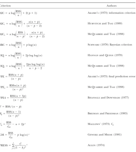
TABLE 2
List of model selection criteria used
Criterion Authors
Akaike’s (1973) information criterion AIC⫽nlog
冢
RSSn
冣
⫹2(p⫹1)HurvitchandTsai(1989) AICc⫽nlog
冢
RSS n
冣
⫹n(n⫹p) (n⫺p⫺2)
McQuarrieandTsai(1998) AICu⫽nlog
冢
RSS n⫺p
冣
⫹n(n⫹p) (n⫺p⫺2)
Schwarz(1978) Bayesian criterion SBC⫽nlog
冢
RSSn
冣
⫹plog(n)HannanandQuinn(1979) HQ⫽nlog
冢
RSSn
冣
⫹2plog log(n)McQuarrieandTsai(1998) HQc⫽nlog
冢
RSS n
冣
⫹2pnlog log(n) n⫺p⫺2
Akaike’s (1973) final prediction error FPE⫽RSS(n⫹p)
(n⫺p)
McQuarrieandTsai(1998) FPEu⫽
RSSn(n⫹p) (n⫺p)2
BhansaliandDownham(1977) FPE4⫽RSS(n⫹3p)
(n⫺p) s2⫽RSS/(n⫺p)
BreimanandFreedman(1983) Rp⫽
RSS(n⫺1) (n⫺p)2
Mallows’ (1973)Cp Cp⫽
RSS s2
full
⫺n⫹2pa
GewekeandMeese(1981)
GM⫽RSS
s2 full
⫺p log(n)a
Allen(1974)
PRESS⫽
兺
n
j⫽1 e2
j (1⫺hj)2
b
RSS, residual sum of squares;p, number of regression parameters [1 (for intercept)⫹number of markers]; n, number of observations.
as2
fullis the residual variance based on the full model.
be
j⫽Yj⫺Yˆj,hj, is thejth diagonal element of the “hat” matrixX(X⬘X)⫺1X⬘, whereXis the design matrix.
shares a common flanking marker. For estimation in the case tion that the generating or true model is of infinite dimension and/or that the set of candidate models does not contain of nonisolated QTL seeWhittakeret al.(1996). In this article,
we assume that QTL are isolated for simplicity of exposition. the true model. The goal is to select the model that best approximates the true model. In large samples, a selection
Model selection criteria:We use criteria in Table 2 to select
the best-fitting model among candidate models. A very thor- criterion that chooses the model with minimum mean squared error (MSE) is said to be asymptotically efficient. Examples ough and concise review of these criteria can be found in
McQuarrieandTsai(1998). Model selection criteria can be for efficient criteria are AIC, AICc,Cp, final prediction error
(FPE),Rp, and leave-one-out cross-validation (PRESS; Table
broadly classified as either efficient or consistent (McQuarrie
discrep-ancy between true model and selected model. The two most gressor variables are nearly uncorrelated (Weisberg1985, p. 195). Marker data from the same chromosome are correlated, common measures are the Kullback-Leibler discrepancy and
mean squared error. Some efficient measures seek to minimize so simple forward selection is problematic, mainly because the best-fitting submodel is likely to be missed, while spurious the former (e.g., AIC), while others try to minimize the latter
(e.g., FPE). Both discrepancy measures are asymptotically variables may enter the model (Weisberg1985). Particularly, some of the variables selected first may not be included in the equivalent (McQuarrieandTsai1998, p. 7).
Consistent criteria are designed for cases where the true best model (seeMiller1990, p. 48, for a striking example). A genome-wide exhaustive search assures that the best-fitting model has low dimension and is assumed to be among the
candidate models. A consistent criterion identifies the correct model will not be missed, but has the disadvantage of a high computational burden.
model asymptotically (as sample size increases) with
probabil-ity one. Examples are SBC, HQ (HannanandQuinn1979), In this article, we propose a modified forward selection strategy based on an article byGabrielandPun(1979; see HQc, and GM (GewekeandMeese1981; Table 2;McQuarrie
and Tsai 1998). It is not clear, on a priori grounds, which also Miller 1990, p. 64). These authors suggested that in some situations it may be possible to find groups of regressors, type of criterion is more appropriate. The objective of QTL
mapping is to detect as many of the true QTL as possible, within which an exhaustive search is possible. The grouping needs to be such that if two variablesxiandxjare in different while not detecting false QTL,i.e., to find the true genetic
model. If the number of QTL is small, we might expect a groups then their regression sum of squares is additive. This requirement is fulfilled for orthogonal variables. For orthogo-consistent criterion to stand a better chance of correctly
de-tecting QTL, while efficient criteria may perform better in nal groups, performing an exhaustive search over all possible models is equivalent to an exhaustive search per group and is more complex cases. Note, however, that optimality of
differ-ent model selection criteria is based on asymptotic argumdiffer-ents. thus guaranteed to find the best-fitting model, with enormous savings in computational effort. Marker data from different Therefore, in this article we study the small sample behavior
of different criteria by means of simulation. chromosomes are stochastically independent. Thus, in large samples, they are nearly orthogonal, conditional on the ob-In case there are more markers than observations, the full
model is not estimable, and hence Mallows’Cpand GM are served data. This suggests that it is useful to do an exhaustive
search for each chromosome and that the regression sum of not applicable due to lack of an error variance estimate based
on the full model. We might continue the forward selection squares for markers from different chromosomes is nearly additive. Of course, in small samples we may fail to find the until the error variance estimate stabilizes, but this raises the
best-fitting model due to chance correlation among markers problem of determining when stabilization has taken place.
from different chromosomes. However, the probability of miss-Incidentally, sequentialF-testing will not work for our
proce-ing the best-fittproce-ing model is expected to be very much smaller dure, since models in the sequence are not necessarily nested.
than with simple forward selection. In this article, a model
Subset selection of markers:In what follows, we first point
will be called sign consistent if its estimated regression coeffi-out the need to select adjacent pairs of markers rather than
cients are of the same sign for each marker pair in the model. individual markers. We then make a few remarks regarding
Our MPS procedure is described as Algorithm 1. applicability of standard subset selection procedures to our
problem. Finally, suggestions are given for modifications
ex-Algorithm1: Make the following definitions:icis a counter ploiting the biology of the problem at hand and the procedure
for the number of marker pairs selected for thecth chromo-is described in algorithmic form.
some; kis the total number of marker pairs in the current The effect and position of a QTL can be estimated from
model;Cis the total number of chromosomes; RSSminis the
the regression coefficients of two flanking markers. A subset
smallest residual sum of squares of sign-consistent models of selection procedure can be used to find markers, which are
orderkfound so far;Mkis the selected model of orderk. likely to flank a QTL. If one marker is selected, we will also
have to include one of the adjacent markers, because two 1. For each chromosome seti
c⫽0. Setk⫽0. Fit the model flanking markers are needed in the estimation procedure. with just an intercept and record the residual sum of Whittakeret al.(1996) state that “an exception to this rule squares (RSS
total). Record this model asM0.
might be when markers are fitted as cofactors to absorb the 2. Setk⇒k⫹1. Set RSS
min⫽RSStotal(from step 1). Forc⫽
effect of QTL which, although too small to be mapped individ- 1 toCdo the following: From the current model drop the ually, contribute a significant portion of genetic variance.” In i
cmarker pairs from thecth chromosome (but keep all pairs our procedure, we include pairs of adjacent markers as a from other chromosomes) and do an exhaustive search for general rule. An obvious requirement for entry of a pair of models withi
c⫹1 marker pairs from thecth chromosome. adjacent markers into the model is that the sign of their Consider entry of a set ofi
c⫹1 pairs of markers only if estimates be the same, for otherwise the estimated model is the resulting model is sign consistent. For a current model not consistent with the presence of a QTL between the pair that is sign consistent, compute the residual sum of squares
(Whittakeret al.1996). (RSS
current). If RSScurrent⬍RSSminthen set RSSmin⫽RSScurrent,
Since we are in a multiple regression framework, standard setc
min⫽c, and record the current model asMk.
procedures for subset selection could be used, such as forward 3. If in step 2 no sign-consistent model of orderk can be selection, etc. (Miller1990; Draperand Smith1998). By found, stop. Else setic⇒ic⫹1 for chromosomecminand so doing, however, we would ignore all we know about the go back to step 2.
relationship among markers. A potential payoff is expected 4. Apply a model selection criterion to select the best-fitting if this knowledge is taken into account. Backward selection is model in the sequence of modelsM
k(k ⫽0, 1, 2 . . . ) not used here, because it does not work when the number of generated by steps 1, 2, and 3.
markers exceeds the sample size. If the number of markers
is large, an overall exhaustive search is usually prohibitive due A remark regarding step 2 is in order. If a sign inconsistency is observed for a pair of markers to be entered, this suggests to the large number of possible models. Forward selection or
“stepwise” regression (Efroymson1960) are the most feasible that the pair may not flank a QTL. Thus, such pairs should not be considered. Checking sign consistency upon entry does approaches among standard techniques. It is well known,
re-allowing a maximum of two QTL per chromosome to limit
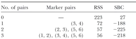
TABLE 3
the computational burden of the exhaustive search. This does
Hypothetical MPS model fitting sequence (n⫽200) not imply, however, that such limitation is needed in practical
applications where there is only one sequence of models to
No. of pairs Marker pairs RSS SBC p be generated instead of 100 or more in simulations. A QTL
was considered as detected when an estimated QTL position
0 — 223 27 1 was within 15 cM of the true QTL position. While the 15-cM
1 (3, 4) 72 ⫺188 3 margin is somewhat arbitrary, rankings of model selection
2 (2, 3), (5, 6) 57 ⫺225 5 criteria according to different performance measures were
3 (1, 2), (3, 4), (5, 6) 56 ⫺218 7 rather insensitive to changes in the margin. If thehth QTL
is detected,␣ˆhis the estimate of thehth QTL effect based on RSS, residual sum of squares; SBC, Schwarz Bayesian crite- (8). Otherwise␣
ˆh⫽ 0. As an aggregate measure of bias we
rion;p, number of parameters. computed
SSE(␣)⫽
兺
Hh⫽1
(␣ˆh⫺ ␣h)2, (10) added, a sign change occurs in a pair from another
chromo-some, that pair may be a false positive, suggesting there is an
where␣ˆhis an estimate of thehth QTL effect. For each model increasing risk of detecting false positives and that the
selec-selection criterion we counted the number of correctly de-tion procedure should be terminated. Therefore, we stop the
tected QTL as well as the number of false positives. From selection process when no sign-consistent model of orderkis
these counts we computed the fraction of correct detections found.
among all detections. If for a given QTL there were more We should point out that it is impossible that different
than one pair yielding a QTL position estimate within 15 cM orders of chromosomes lead to different results with
Algo-of the true QTL position, only the pair with position estimate rithm 1. This is because step 2 tries to add a pair of markers
closest to the true QTL was considered as a detecting pair. on each chromosome. In step 3 the algorithm then chooses
All pairs of markers not detecting any QTL were considered the one chromosome for which addition of a pair gives the
as false positives. best fit. This will be the same chromosome, regardless of the
We considered 14 examples with different QTL numbers, order in which chromosomes are tried.
positions, and effect sizes (Table 4). Heritabilities were com-Note that in the model sequence obtained from Algorithm
puted as described in theappendix. Example 1 is adapted 1, the best model withkpairs does not necessarily contain all
fromLanderandBotstein(1989). In this example, there are markers that are in the best model withk⫺1 pairs or less.
five QTL with decreasing effect size. This pattern of “tapered An important reason for allowing the implicit drop of one or
effects” (BurnhamandAnderson1998),i.e., few large effects two markers during each step of the model-building process
and many small effects, is very typical of many real applications is that there may be two adjacent QTL on the same
chromo-(Kearsey and Farquhar 1998). Lander and Botstein some with the same sign of the associated genetic effect. The
(1989) used a marker spacing of 20 cM for IM. FromDarvasi pair of markers selected first is likely to lie between the two
et al. (1993) andPiepho(2000) it can be conjectured that QTL. If left in the model, a ghost QTL will be detected.
using a much smaller spacing does not usually provide a dra-Allowing a pair to be dropped from the model during model
matic gain in accuracy and power for loosely linked QTL. building reduces the risk of detecting ghost QTL. For a
chro-For detecting closely linked QTL, however, a finer spacing is mosome with six markers and two QTL in the intervals (2, 3)
necessary. In all examples except two, we used a spacing of and (5, 6) the model sequence may look like the hypothetical
10 cM. We also included one example with a spacing of 5 cM. example shown in Table 3. The first pair tries to explain as
We do not consider finer marker spacings since this would much of the phenotypic variation as possible. However, only
increase the problem of multicollinearity and thus of instabil-marker 3 is a flanking instabil-marker. Marker 4 is included because
ity of parameter estimates (Melchinger et al. 1998). The it accounts for the QTL in the interval (5, 6). In the next step,
LanderandBotstein(1989) example was modified in differ-marker 4 is dropped while the flanking pairs (2, 3) and (5,
ent ways,i.e., by changing of error variance (heritability) and 6) enter. SBC selects the four-marker model as fitting best
marker spacing. We included some other examples with less (smallest value of criterion), while the full model fits slightly
and with more markers. Examples 9 and 10 are adapted from worse. Were simple forward selection applied to the above
Beavis (1994), who used examples with 10 and 40 QTL of example, we would first select the pair (3, 4), and this would
the same, but small effect. Also, examples with two QTL on remain in the model throughout. Thus, there is no more
the same chromosome were included (examples 7, 8, 13, and flexibility to end up with the “true” marker model (2, 3, 5,
14; see Table 4). 6), and a ghost QTL will be detected.
If markers are densely spaced, it may happen that two
adja-Simulation study:We simulated BC1populations for various
cent markers are perfectly correlated, so that the design matrix settings. The number of chromosomes ranged from 12 to 20,
for a model that includes these two markers is not of full while the number of QTL was between zero and five. Equal
column rank. If two markers are perfectly correlated, there is spacing of markers (10 or 20 cM) along a 100-cM chromosome
no information as to the position and effect of a QTL between and absence of interference were assumed. The number of
the markers and the approach of Whittakeret al. (1996) crossovers per chromosome was simulated according to a
Pois-breaks down, unless some constraint is imposed. For simplicity, son distribution with parameter equal to the length of the
we rejected the corresponding model in simulations. The chromosome in morgans, which is in accordance with
Hal-problem occurred very rarely with a marker spacing of 10 cM dane’s mapping function. For each setting, we performed 100
and never with a marker spacing of 20 cM, but became more simulation runs. Assuming Poisson sampling, the standard
serious with spacings of 5 cM and smaller (results not shown). error for an expected count(e.g., number of false positives)
In practice one would include a check for collinearity ( Sari-is (/100)0.5,e.g., 0.2 for ⫽4. Due to high positive correlation
Gorlaet al.1997), drop one of two perfectly (or very highly) among statistics of the same type as computed for different
correlated markers, and include the best fitting of either adja-selection criteria (number of false positives, etc.), the accuracy
TABLE 4
Examples considered in simulations of BC1populations
Example QTL (chromosome, position, effect) h2 C M L D 2
1 (1, 71, 1.5), (2, 49, 1.25), (3, 27, 1.0), (4, 8, 0.75), (5, 31, 0.5) 0.58 12 200 100 20 1
2 (1, 71, 1.5), (2, 49, 1.25), (3, 27, 1.0), (4, 8, 0.75), (5, 31, 0.5) 0.58 12 200 100 10 1
3 (1, 71, 1.5), (2, 49, 1.25), (3, 27, 1.0), (4, 8, 0.75), (5, 31, 0.5) 0.82 12 200 100 10 0.3
4 (1, 71, 1.5), (2, 49, 1.25), (3, 27, 1.0), (4, 8, 0.75), (5, 31, 0.5) 0.32 12 200 100 10 3
5 (1, 71, 1.5), (2, 49, 1.25), (3, 27, 1.0), (4, 8, 0.75), (5, 31, 0.5) 0.58 12 500 100 10 1
6 (1, 24, 1.5), (1, 56, 1.25), (3, 27, 1.0), (4, 8, 0.75), (5, 31, 0.5) 0.66 12 200 100 10 1
7 (1, 24, 1.5), (1, 56, 1.25) 0.59 12 200 100 10 1
8 (1, 24, 1.5), (1, 56,⫺1.25) 0.31 12 200 100 10 1
9 (c, 55, 0.5) forc⫽1, . . . , 12 0.43 12 200 100 10 1
10 (c, 55, 0.5) forc⫽1, . . . , 12 0.71 12 200 100 10 0.3
11 (1, 71, 1.5) 0.36 12 200 100 10 1
12 — 0 12 200 100 10 1
13 (1, 24, 1.5), (1, 56, 1.25) 0.59 20 200 100 10 1
14 (1, 24, 1.5), (1, 56, 1.25) 0.59 12 200 100 5 1
h2, heritability;C, number of chromosomes;M, number of individuals;L, length of chromosome;D, marker spacing;2, error
variance.
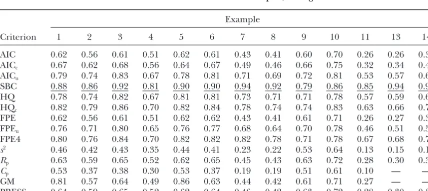
RESULTS age of correct detections among all detections (Table
7), often followed by HQcand FPE4. For these two types
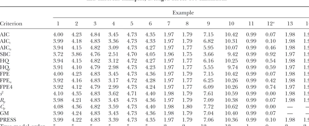
The number of detected QTL is usually quite stable
of counts, SBC is generally markedly superior to some across criteria (Table 5). SBC tends to select the simplest
other quite popular criteria such ass2andC
p. For
exam-models and thus the average number of correctly
de-ple, with example 2, SBC has an average number of tected QTL is usually smaller than for other criteria,
0.63 false detections, whiles2andC
phave 6.06 and 7.36
but the difference is very small most of the time, except
false detections, respectively. SBC is followed by HQc
for more extreme cases such as examples 9 and 10,
(1.07) and FPE4 (1.31) in this example. In the example where the difference is somewhat more pronounced.
with no QTL (example 12), SBC picks the correct model
HQc and FPE4 also tend to select simpler models. In
(model with no markers) 92% of the time, which is by all cases investigated, SBC clearly has the smallest false
positive rate (Table 6) and the most favorable percent- far better than any other criterion. Only FPE4 and HQc
TABLE 5
Number of true QTL detected by MPS for selected fitted models based on different selection criteria and different examples, averaged across 100 simulations
Example
Criterion 1 2 3 4 5 6 7 8 9 10 11 12a 13 14
AIC 4.00 4.23 4.84 3.45 4.73 4.35 1.97 1.79 7.15 10.42 0.99 0.07 1.98 1.97
AICc 3.99 4.18 4.83 3.36 4.73 4.33 1.97 1.79 6.82 10.31 0.99 0.10 1.98 1.97
AICu 3.94 4.15 4.82 3.09 4.73 4.27 1.97 1.77 5.95 10.07 0.99 0.46 1.98 1.97
SBC 3.72 3.86 4.76 2.51 4.70 4.05 1.96 1.75 3.66 9.42 0.99 0.92 1.97 1.97
HQ 3.94 4.15 4.82 3.12 4.72 4.27 1.97 1.77 6.16 10.25 0.99 0.54 1.98 1.97
HQc 3.91 4.10 4.79 2.98 4.73 4.23 1.97 1.77 5.55 9.74 0.99 0.59 1.97 1.97
FPE 4.00 4.23 4.83 3.45 4.73 4.36 1.97 1.79 7.15 10.42 0.99 0.07 1.98 1.97
FPEu 3.92 4.16 4.83 3.17 4.72 4.28 1.97 1.77 6.25 10.26 0.99 0.42 1.98 1.97
FPE4 3.92 4.12 4.79 2.99 4.73 4.24 1.97 1.77 6.09 10.26 0.99 0.74 1.97 1.97
s2 4.10 4.35 4.83 3.62 4.71 4.40 1.98 1.79 7.61 10.59 0.99 0.00 1.98 1.97
Rp 3.98 4.21 4.83 3.43 4.73 4.36 1.97 1.79 7.09 10.38 0.99 0.07 1.98 1.97
Cp 4.08 4.36 4.82 3.59 4.73 4.40 1.98 1.80 7.72 10.62 0.99 0.00 — —
GM 3.90 4.24 4.83 3.43 4.73 4.36 1.98 1.79 7.04 10.40 0.99 0.07 — —
PRESS 3.99 4.22 4.83 3.39 4.73 4.35 1.97 1.79 7.06 10.36 0.99 0.10 1.98 1.97
True model order 5 5 5 5 5 5 2 2 12 12 1 0 2 2
The different examples are described in Table 4.
TABLE 6
Number of false positives among detections for fitted models selected by MPS based on different selection criteria and different examples, averaged across 100 simulations
Example
Criterion 1 2 3 4 5 6 7 8 9 10 11 12 13 14
AIC 2.50 3.32 3.12 3.37 2.95 2.81 2.63 2.56 4.68 4.44 2.82 2.99 5.50 4.28
AICc 1.93 2.53 2.30 2.66 2.71 2.11 2.08 2.07 3.56 3.40 2.12 2.42 3.76 2.86
AICu 1.07 1.44 0.98 1.49 1.34 0.98 0.80 0.79 2.32 2.32 0.88 0.85 1.48 1.15
SBC 0.51 0.63 0.44 0.58 0.51 0.44 0.12 0.16 0.97 1.59 0.17 0.10 0.13 0.14
HQ 1.09 1.48 1.05 1.56 1.11 1.01 0.73 0.72 2.54 2.86 0.75 0.68 1.36 1.08
HQc 0.86 1.07 0.78 1.26 1.01 0.82 0.54 0.63 1.97 2.01 0.58 0.52 1.02 0.66
FPE 2.48 3.31 3.08 3.37 2.95 2.67 2.62 2.54 4.65 4.34 2.82 2.99 5.34 4.25
FPEu 1.27 1.66 1.19 1.74 1.50 1.31 0.94 0.99 2.72 2.91 1.15 0.94 1.90 1.41
FPE4 0.95 1.31 0.91 1.29 1.02 0.92 0.43 0.50 2.45 2.88 0.49 0.34 0.94 0.63
s2 4.84 6.06 6.35 6.73 6.11 6.34 6.68 6.30 6.65 5.93 6.63 7.60 11.11 9.35
Rp 2.30 2.91 2.61 3.12 2.87 2.36 2.45 2.40 4.15 3.97 2.49 2.74 4.55 3.77
Cp 3.58 7.36 7.72 8.31 4.26 7.35 8.24 7.73 7.45 6.91 8.48 9.08 — —
GM 0.92 3.26 2.67 3.58 0.80 2.58 2.56 2.46 4.41 4.30 2.73 2.94 — —
PRESS 2.26 2.88 2.61 3.09 2.88 2.46 2.33 2.51 4.17 3.96 2.58 2.89 4.56 3.43
The different examples are described in Table 4.
come anywhere near this figure (59 and 74%, respec- criteria such as AIC, are extreme cases in many respects.
The effects are all equal and not tapered as in many of tively). It should be noted that all criteria select from
the same sequence of models. The difficult task is to the other examples. In contrast to other examples, SBC
has a markedly smaller number of correct detections in strike the right balance between underfitting and
over-fitting,i.e., to find Ockham’s Hill (MacKay1992), and example 9 (Table 5), so the fact that it still has the most favorable rate of correct detections relative to the total it is this task for which model selection criteria are
de-signed. Obviously, SBC is best at finding a suitable cut- number of detections does not have an unambiguous
interpretation. If we are more concerned about false off;i.e., it detects when the sequence starts picking up
more noise than pattern. positives, SBC is clearly favorable, while other criteria
fare better regarding the number of correct detections. Examples 9 and 10, which were chosen mainly to see
how the criteria performing best in most cases would Examples 13 and 14 have the same QTL as example
7, but are different in that the number of markers ex-perform under circumstances very favorable to other
TABLE 7
Proportion of number of detected true QTL among total number of detections for fitted models selected by MPS based on different selection criteria and different examples, averaged across 100 simulations
Example
Criterion 1 2 3 4 5 6 7 8 9 10 11 13 14
AIC 0.62 0.56 0.61 0.51 0.62 0.61 0.43 0.41 0.60 0.70 0.26 0.26 0.32
AICc 0.67 0.62 0.68 0.56 0.64 0.67 0.49 0.46 0.66 0.75 0.32 0.34 0.41
AICu 0.79 0.74 0.83 0.67 0.78 0.81 0.71 0.69 0.72 0.81 0.53 0.57 0.63
SBC 0.88 0.86 0.92 0.81 0.90 0.90 0.94 0.92 0.79 0.86 0.85 0.94 0.93
HQ 0.78 0.74 0.82 0.67 0.81 0.81 0.73 0.71 0.71 0.78 0.57 0.59 0.65
HQc 0.82 0.79 0.86 0.70 0.82 0.84 0.78 0.74 0.74 0.83 0.63 0.66 0.75
FPE 0.62 0.56 0.61 0.51 0.62 0.62 0.43 0.41 0.61 0.71 0.26 0.27 0.32
FPEu 0.76 0.71 0.80 0.65 0.76 0.77 0.68 0.64 0.70 0.78 0.46 0.51 0.58
FPE4 0.80 0.76 0.84 0.70 0.82 0.82 0.82 0.78 0.71 0.78 0.67 0.68 0.76
s2 0.46 0.42 0.43 0.35 0.44 0.41 0.23 0.22 0.53 0.64 0.13 0.15 0.17
Rp 0.63 0.59 0.65 0.52 0.62 0.65 0.45 0.43 0.63 0.72 0.28 0.30 0.34
Cp 0.53 0.37 0.38 0.30 0.53 0.37 0.19 0.19 0.51 0.61 0.10 — —
GM 0.81 0.57 0.64 0.49 0.86 0.63 0.44 0.42 0.61 0.71 0.27 — —
PRESS 0.64 0.59 0.65 0.52 0.62 0.64 0.46 0.42 0.63 0.72 0.28 0.30 0.36
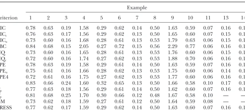
TABLE 8
SSE(␣) for fitted models selected by MPS based on different selection criteria and
different examples, averaged across 100 simulations
Example
Criterion 1 2 3 4 5 6 7 8 9 10 11 13 14
AIC 0.78 0.63 0.19 1.58 0.29 0.62 0.14 0.50 1.63 0.59 0.07 0.16 0.18
AICc 0.76 0.63 0.17 1.56 0.29 0.62 0.13 0.50 1.65 0.60 0.07 0.15 0.18
AICu 0.73 0.60 0.16 1.68 0.28 0.61 0.13 0.53 1.79 0.63 0.06 0.15 0.16
SBC 0.84 0.68 0.15 2.05 0.27 0.72 0.15 0.56 2.29 0.77 0.06 0.16 0.16
HQ 0.73 0.60 0.16 1.65 0.28 0.61 0.13 0.53 1.76 0.60 0.06 0.15 0.16
HQc 0.72 0.60 0.16 1.74 0.27 0.62 0.13 0.53 1.88 0.70 0.06 0.16 0.16
FPE 0.78 0.63 0.19 1.58 0.29 0.61 0.14 0.50 1.63 0.59 0.07 0.16 0.18
FPEu 0.75 0.61 0.16 1.66 0.28 0.62 0.13 0.53 1.75 0.60 0.06 0.14 0.16
FPE4 0.72 0.61 0.16 1.75 0.27 0.62 0.13 0.53 1.77 0.60 0.06 0.16 0.16
s2 0.83 0.66 0.24 1.60 0.32 0.65 0.13 0.50 1.66 0.58 0.10 0.17 0.18
Rp 0.77 0.63 0.18 1.56 0.29 0.61 0.14 0.50 1.62 0.60 0.07 0.16 0.18
Cp 0.81 0.68 0.25 1.70 0.30 0.66 0.12 0.48 1.67 0.58 0.10 — —
GM 0.73 0.62 0.18 1.59 0.27 0.61 0.12 0.50 1.64 0.59 0.08 — —
PRESS 0.77 0.62 0.17 1.59 0.29 0.62 0.14 0.50 1.63 0.60 0.07 0.16 0.18
The different examples are described in Table 4.
ceeds the number of individuals. Thus, there is a larger ples, mainly due to undetected QTL. Bias decreases with
smaller variance2(examples 2–4 and examples 9 and
potential for overfitting. Note that the criteria Cpand
10). This corroborates the finding of Utz and
Mel-GM are not applicable because the number of markers
chinger (1994) that heritability is among the main exceeds the sample size. While for both examples 13
factors determining bias. Our results for examples 9 and 14 the number of correct detections is about the
and 10 are somewhat more diverse than those ofBeavis
same for all criteria, SBC is the clear winner in terms
(1994), who almost exclusively found large upward bi-of the ratio bi-of true detections among all detections
ases for examples similar to ours on the basis of a compa-(Table 7). For many of the other criteria, the number
rable range of heritabilities. Note that Beavis (1994)
of false detections (Table 6) increases dramatically for
used IM, which has been shown by Utz and
Mel-examples 13 and 14 compared to example 7, showing
chinger(1994) to be associated with more severe biases that the problem of overfitting increases with the
num-than CIM. We should point out that MPS is more akin ber of markers. SBC is the only criterion for which the
to CIM, which may go some way toward explaining the number of false positives does not change markedly
contrasting results. Moreover, bias assessment is neces-relative to example 7.
sarily somewhat arbitrary, for it depends on the defini-A comparison of examples 2, 3, 4, and 5 in Tables 6
tion of QTL detection. We consider a QTL as detected and 7 shows that all criteria select simpler models as2
when the model has a position estimate within 15 cM increases and as sample size decreases. Increasing the
from the true QTL. Changing the margin to 10 or 20 sample size from 200 (example 2) to 500 (example 5)
cM leads to different bias estimates. results in a mild increase in the number of correct
We summarize the results as follows: Since the num-detections (Table 5) and in the proportion of correct
ber of correct detections is usually quite constant across detections among all detections (Table 7). Reducing
criteria, we think that the number of false positives and marker spacing (compare examples 1 and 2 and
exam-the fraction of correct detections are exam-the most meaning-ples 7 and 14) increased the number of false positives
ful performance measures. From the overall picture of and reduced the proportion of correct detections,
indi-simulation results, SBC emerges as the best criterion, cating that the risk of overfitting increases with the
num-with FPE4 and HQc as the closest competitors. While
ber of markers. Note, however, that in example 2 the
SBC, HQc, and FPE4 tend to find slightly fewer QTL
number of correct detections is also increased relative
than other criteria, they do much better in avoiding the to example 1.
risk of detecting spurious QTL. Bias, as assessed by the overall measure SSE(␣), is
comparable for all selection criteria (Table 8). The only exception to this rule is SBC, which due to its tendency
DISCUSSION
to select simpler models than other criteria has a notably
smaller number of detected QTL and so has somewhat Features of MPS: MPS is a new procedure that
exam-while limiting the risk of detecting spurious QTL. It IM/CIM finds the QTL. Our procedure can be modified to account for the problem. Consider three adjacent contains three important building blocks specifically
designed to achieve this goal: (i) selection of marker markers 1, 2, and 3 and assume there is a QTL close to
marker 2. As we scan the chromosome, adjacent pairs pairs, (ii) augmentation of a forward selection
proce-dure by an exhaustive search per chromosome, and (iii) (1, 2) and (2, 3) will be tried, possibly in conjunction
with a set of additional pairs on the same chromosomes. application of a model selection criterion to select the
final model from a sequence of models. None of these We suggest scrutinizing fits of pairs (1, 2) and (2, 3)
with the same set of additional pairs on the same chro-building blocks is in itself new. The novelty here is the
way in which these components are integrated into a mosome (this set may be empty). If the sign of the
regression coefficient for marker 2 is the same for both single algorithm and how they are applied to QTL
map-ping, exploiting our knowledge of the underlying biol- pairs, and if the signs of regression coefficients for
mark-ers 1 and 3 agree with each other and are opposite to ogy. The two main differences between MPS and CIM
are the way in which cofactors are selected and how the the sign for marker 2, the QTL would go unnoticed by
Algorithm 1. Thus, in such cases we could fit the pair final model is selected. MPS implicitly uses marker pairs
of other QTL as cofactors, while conventional CIM can (1, 3), again with the same set of additional pairs. The
pair (1, 3) would be considered further only if the signs use a wide variety of ways in which cofactors are selected
(forward selection, using the best five markers, using of the regression coefficients for markers 1 and 3 change
compared to the corresponding fits with pairs (1, 2) two markers per chromosome, etc.). MPS uses criteria
such as SBC to select a model, while CIM uses multiple and (2, 3). If the pair (1, 3) is selected for the current
model order, the dropped marker 2 could be con-LR tests.
MPS can be used as a stand-alone procedure for de- sidered again for higher model orders. We have not
incorporated this modification in our description of tecting QTL and estimating their effect and position in
BC1 populations, or equivalently for recombinant in- Algorithm 1 and in the simulation, because in our
expe-rience the problem is not very common, and the ex-bred and doubled haploid lines. It is also applicable
for F2populations, if one is interested only in additive pected gain in power is small. Also, the modification
increases the risk of detecting false positives. effects, but not in dominance effects (Whittakeret al.
1996). Alternatively, for any kind of unselected popula- Instead of an exhaustive search per chromosome as
implemented in our Algorithm 1, we could adopt a tion, MPS may serve as a supplement to CIM in two
ways. First, the LOD profile produced by CIM can be simple forward selection procedure, possibly improved
by some measures to exploit knowledge of the biology. overlaid with the positions of the pairs of markers
se-lected by MPS. Peaks in the profile associated with se- For example, if at one step markers 2 and 3 have been
selected on a chromosome, it is sensible to allow the lected pairs can then be given more credibility than
other peaks. Second, MPS can be used to select cofac- pair (1, 4) to be selected in subsequent steps, providing
pairs (1, 2) and (3, 4) lead to regression estimates of tors. While Algorithm 1 will likely select pairs of markers
accounting for QTL, it may not be efficient to use all the same sign for a pair. This makes sure that the
“cor-rect” pairs can be selected in case there are two isolated markers selected by Algorithm 1 in CIM. Instead, it may
be preferable to use only a subset of markers selected QTL in the intervals (1, 2) and (3, 4) on the same
chromosome, and at an earlier step pair (2, 3) was by Algorithm 1. We therefore suggest using the markers
detected by Algorithm 1 and performing an exhaustive selected. Also, we could allow a selected pair of markers
to move one position to the left or to the right as more search, using some model selection criterion. The
re-sulting subset may be submitted to CIM. It is as yet marker pairs are being added. Thus,e.g., having selected
the pair (2, 3) at some stage, we would allow this pair an open question whether use of all pairs of markers
selected by Algorithm 1 in CIM is inferior to using a to be replaced by (1, 2) or (3, 4) later in the selection
process, if this improves the fit. One can think of more subset of them. This question deserves further study.
The equivalence of IM/CIM as applied to adjacent modifications of simple forward selection. In fact, the
modified algorithm may become fairly complicated and
marker pairs and the approach by Whittaker et al.
(1996) used in MPS is restricted to the case where IM/ unrealistic to program when one attempts to cover all
the possible QTL and marker configurations that may CIM does not map a QTL exactly at a marker,i.e., where
the RSS has a local minimum in the open intervalrL苸 occur in reality. While our partially exhaustive search
is computationally more demanding, it has the virtue (0,) and this minimum is smaller than the RSS atrL⫽
0 andrL ⫽ . In our experience this case will be the of simplicity and at the same time covers many of the
features lacking in a simple forward selection algorithm. rule in real applications. As pointed out by a referee, if
IM/CIM maps a true QTL exactly at a marker, it is We observed that occasionally MPS selects more than
one pair of markers for a large QTL, leading to
overfit-possible that with the approach of Whittaker et al.
(1996) estimates ofLandRhave opposite sign, where ting of that QTL. We could augment our Algorithm 1
by a step that tries to reduce the model whenever there one marker corresponds to the mapped QTL. In this
case it may happen that Algorithm 1 fails to detect the are two or more pairs of markers on the same
that this modification will slightly increase efficiency Further remarks on model selection:Procedures for mapping QTL aim at finding as many true QTL as when in fact there is only one QTL on the chromosome,
while it may deteriorate performance of the algorithm possible, while avoiding the risk of detecting spurious
QTL. Significance testing as is commonly used for IM, in case there is more than one QTL. We have not
in-cluded such modifications in our simulation study for CIM, and MIM is not necessarily the best strategy to
achieve this goal (GelfandandGhosh1998). For IM,
simplicity.
Comparison of MPS to other procedures:In conven- there are a number of methods for determining the appropriate threshold so that the genome-wise type I tional CIM, cofactors are usually selected on the basis
of simple forward selection, with markers entering the error rate is controlled at a predetermined value, such
as 5% (LanderandBotstein1989, 1994;Churchill
model individually rather than in pairs. Often, the
selec-tion is semiautomated or fully automated, with no check andDoerge1994;Rebaı¨et al.1994, 1995;Doergeand
Churchill1996;GoffinetandMangin1998;Dupuis
of whether or not the selected cofactors match QTL
detected later in the CIM scan across the chromosome. and Siegmund1999). Most of these methods operate
under a global null hypothesis of no QTL anywhere in Such a check would be useful as a guard against
overfit-ting. It has been observed that inclusion of too many the genome, which is rather restrictive, but seeDoerge
and Churchill (1996) and Goffinet and Mangin
cofactors that are not associated with a QTL will reduce
power to identify QTL relative to IM (Zeng1993;Beavis (1998). Controlling the genome-wise error rate in a
sequential model-building process is an inherently dif-1994). Since MPS selects markers in pairs, the likelihood
of selecting spurious markers as cofactors is reduced. ficult problem. Also, significance tests do not allow a
comparison of nonnested models. Forcing a nested Moreover, a stringent criterion such as SBC further
re-duces the risk of overfitting. model sequence entails the risk of detecting ghost QTL
and missing better-fitting models. Moreover, having A more detailed comparison of CIM and MPS would
be rewarding, but is beyond the scope of this article. controlled the genome-wise rate of false positives among
tests under the null hypothesis of no QTL at 5%, the For CIM there are many parameters that would have to
be considered in simulations: window size, definition of rate of false positives among QTL detections, which is a
different quantity that is usually of greater interest, can critical threshold, definition of when a LOD peak
de-tects a QTL and when it must be considered as a “sub- easily be 50% or more (SoutheyandFernando1998).
peak” of another detecting peak, selection of cofactors, Model selection criteria are based on a philosophy
ML, or least squares, etc. In fact, CIM could be modified that is essentially different from that underlying
signifi-by taking up some or all of the ingredients that make cance testing (BurnhamandAnderson1998). A
com-up MPS,i.e., selecting markers in pairs, requiring sign mon basis of many criteria is the notion that the more
consistency, using SBC or some other criterion instead information is gathered, the greater is the model
com-of LOD thresholds, doing an exhaustive search per chro- plexity that the data can support (Bucklandet al.1997).
mosome to select cofactors, etc. Thus, a detailed com- While not guaranteeing the absence of false positives
parison will have to be fairly extensive and should in- among detections, criteria such as SBC do a better job
clude various blends of MPS and CIM. Such a study is at striking the balance between the contrasting
objec-left for future work. tives of finding as many real QTL as possible and at the
Recently, Kao et al. (1999) suggested a method same time keeping the risk of fitting spurious QTL low.
termed multiple interval mapping (MIM) that was Moreover, the difficult task of finding an appropriate
judged superior to CIM. Using MIM, several QTL can adjustment for multiple testing to control a
genome-be fitted simultaneously, allowing for complex models wise error rate is obviated, and nonnested models can
of gene action including epistasis. Due to the potentially be compared.
large complexity of models fitted by MIM, there is a In this article we have not used computer-intensive
severe danger of overfitting. The authors mention a methods of model selection, such as leave-d-out cross
number of model selection strategies, including use of validation and bootstrapping (Hjorth1994;
McQuar-AIC and SBC, but, for their suggested procedure, they rieandTsai1998), to limit the computational burden
adopt a stepwise selection procedure in conjunction in simulations. It is interesting to note, however, that
with multiple LR testing and a Bonferroni adjustment there exist several asymptotic equivalence relationships
on tests for epistasis. The results presented in our article between cross-validation and selection criteria used here
strongly suggest that the performance of MIM could be (see Table 2), for example, between FPE and PRESS as
considerably improved by using a selection criterion well as between SBC and leave-d-out cross validation,
such as SBC in place of multiple LR tests. In fact, MPS whend⫽n(1⫺1/(log(n)⫺1)) (Shao1996;
McQuar-can be used to first select potential regions in the ge- rieandTsai1998).
nome for fitting QTL. This can be followed by MIM
Lander, E. S.,andD. Botstein,1989 Mapping Mendelian factors New York. Support of the Heisenberg Programm of the Deutsche
underlying quantitative traits using RFLP linkage maps. Genetics Forschungsgemeinschaft is gratefully acknowledged.
121:185–199.
Lander, E. S.,andD. Botstein,1994 Corrigendum. Genetics136:
705.
Lebreton, C. M.,andP. M. Visscher,1998 Empirical nonparamet-LITERATURE CITED
ric bootstrap strategies in quantitative trait loci mapping: condi-tioning on the genetic model. Genetics148:525–535. Akaike, H.,1973 Information theory and an extension of the
maxi-mum likelihood principle, pp. 267–281 in2nd International Sympo- MacKay, D. J. K.,1992 Bayesian interpolation. Neural Comput.4:
415–447.
sium on Information Theory, edited byB. N. PetrivandF. Csaki.
Aakademia Kiado, Budapest. Mallows, C. L.,1973 Some comments on Cp. Technometrics15:
661–675. Allen, D. M.,1974 The relationship between variable selection and
data augmentation and a method for prediction. Technometrics Martinez, O.,andR. N. Curnow,1992 Estimating the locations and the sizes of the effects of quantitative trait loci using flanking
16:125–127.
Beavis, W. D.,1994 The power and deceit of QTL experiments: markers. Theor. Appl. Genet.85:480–488.
McQuarrie, A. D. R.,andC.-L. Tsai,1998 Regression and Time Series
lessons from comparative QTL studies, pp. 250–266 inReport of
the Forty-Ninth Annual Corn and Sorghum Research Conference, edited Model Selection.World Scientific Publishers, Singapore. Melchinger, A. E., H. F. UtzandC. C. Scho¨ n,1998 Quantitative byD. B. Wilkinson.American Seed Trade Association,
Washing-ton, DC. trait loci (QTL) mapping using different testers and independent
population samples in maize reveals low power of QTL detection Bhansali, R. J., andD. Y. Downham, 1977 Some properties of
the order of an autoregressive model selected by a generalized and large bias in estimates of QTL effects. Genetics149:383–403. Miller, A. J.,1990 Subset Selection in Regression.Chapman & Hall, Akaike’s EPF criterion. Biometrika64:547–551.
Breiman, L.,andD. Freedman,1983 How many variables should be London.
Piepho, H. P.,2000 Optimal marker density for interval mapping entered in a regression equation? J. Am. Stat. Assoc.78:131–136.
Buckland, S. T., K. P. BurnhamandN. H. Augustin,1997 Model in a backcross population. Heredity84:437–440.
Rebaı¨, A., B. GoffinetandB. Mangin,1994 Approximate thresh-selection: an integral part of inference. Biometrics53:603–618.
Burnham, K. P.,andD. R. Anderson,1998 Model Selection and Infer- olds of interval mapping tests for QTL detection. Genetics138:
235–240.
ence.Springer, New York.
Churchill, G. A.,andR. W. Doerge,1994 Empirical threshold Rebaı¨, A., B. GoffinetandB. Mangin,1995 Comparing power of different methods for QTL detection. Biometrics51:87–99. values for quantitative trait mapping. Genetics138:963–971.
Darvasi, A., A. Weinreb, V. Minke, J. I. WellerandM. Soller, Sari-Gorla, M., T. Calinski, Z. KaczmarekandP. Krajewski,1997 Detecting QTL⫻environment interaction in maize by a least 1993 Detecting marker-QTL linkage and estimating QTL gene
effect and map location using a saturated genetic map. Genetics squares interval mapping method. Heredity78:146–157. Schwarz, G.,1978 Estimating the dimension of a model. Ann. Stat.
134: 943–951.
Doerge, R. W.,andG. A. Churchill,1996 Permutation tests for 6:461–464.
Shao, J.,1996 Bootstrap model selection. J. Am. Stat. Assoc. 91:
multiple loci affecting a quantitative character. Genetics 142:
285–294. 655–665.
Sillanpa¨a¨, M. J.,andE. Arjas,1998 Bayesian mapping of multiple Draper, N. R.,1995 Assessment and propagation of model
uncer-tainty. J. R. Stat. Soc. B57:45–97. quantitative trait loci from incomplete inbred line cross data. Genetics148:1373–1388.
Draper, N. R.,andH. Smith,1998 Applied Regression Analysis.Wiley,
New York. Southey, B. R.,andR. L. Fernando,1998 Controlling the
propor-tion of false positives among significant results in QTL detecpropor-tion. Dupuis, J.,andD. Siegmund,1999 Statistical methods for mapping
quantitative trait loci from a dense set of markers. Genetics151: Proc. 6th World Congr. Genet. Appl. Livest. Prod.26:221–224. Stam, P.,1991 Some aspects of QTL analysis, pp. 23–31 inProceedings
373–386.
Efroymson, M. A.,1960 Multiple regression analysis, pp. 191–203 of the VIIIth Meeting of the Eucarpia Section Biometrics in Plant Breeding, edited by J.Pesek, M. HermanandJ. Hartmann.Brno, Czecho-inMathematical Methods for Digital Computers, edited byA.
Ral-stonandH. S. Wilf.Wiley, New York. slovakia.
Utz, H. F.,andA. E. Melchinger,1994 Comparison of different Gabriel, K. R.,andF. C. Pun,1979 Binary prediction of weather
events with several predictors, pp. 248–253 in6th Conference on approaches to interval mapping of quantitative trait loci, pp. 195–204 in Biometrics in Plant Breeding: Application of Molecular Probability and Statistics in Atmospheric Sciences.American
Meteoro-logical Society, Boston, MA. Markers,Proceedings of the Ninth Meeting of the EUCARPIA Section
Biometrics in Plant Breeding, edited byJ. W. van Ooijen andJ. Gelfand, A. E.,andS. K. Ghosh,1998 Model choice: a minimum
posterior predictive loss approach. Biometrika85:1–11. Jansen.CPRO-DLO, Wageningen, The Netherlands. Weir, B.,1996 Genetic Data Analysis II.Sinauer, Sunderland, MA. Geweke, J.,andR. Meese,1981 Estimating regression models of
finite but unknown order. Int. Econ. Rev.22:55–70. Weisberg, S.,1985 Applied Linear Regression.Wiley, New York. Whittaker, J. C., R. ThompsonandP. M. Visscher,1996 On the Goffinet, B.,andB. Mangin,1998 Comparing methods to detect
more than one QTL on a chromosome. Theor. Appl. Genet.96: mapping of QTL by regression of phenotype on marker-type. Heredity77:23–32.
628–633.
Haley, C. S.,andS. A. Knott,1992 A simple regression method Zeng, Z.-B.,1993 Theoretical basis of separation of multiple linked gene effects on mapping quantitative trait loci. Proc. Natl. Acad. for mapping quantitative trait loci in line crosses using flanking
markers. Heredity69: 315–324. Sci. USA90:10972–10976.
Zeng, Z.-B.,1994 Precision mapping of quantitative trait loci. Genet-Hannan, E. J.,andB. G. Quinn,1979 The determination of the
order of an autoregression. J. R. Stat. Soc. B41:190–195. ics136:1457–1466. Hjorth, J. S. U.,1994 Computer Intensive Statistical Methods. Validation,
Communicating editor:C. Haley
Model Selection and Bootstrap.Chapman and Hall, London. Hurvitch, C. M.,andC.-L. Tsai,1989 Regression and time series
model selection in small samples. Biometrika76:297–307. Jansen, P. C.,1993 Interval mapping of multiple quantitative trait
APPENDIX loci. Genetics135:205–211.
Jansen, R. C.,andP. Stam,1994 High resolution of quantitative
Let z ⫽ g1␣1 ⫹ g2␣2, where ␣1 and ␣2 are additive
traits into multiple loci via interval mapping. Genetics136:1447–
1455. genetic effects of two QTL andg1 andg2 are coded 0
Kao, C. H., Z-B. ZengandR. D. Teasdale,1999 Multiple interval and 1 depending on the genotype at the QTL. For the mapping for quantitative trait loci. Genetics152:1203–1216.
nonrecombinant genotypes we have eitherg1⫽g2⫽0
Kearsey, M. J.,andA. G. L. Farquhar,1998 QTL analysis in plants:
andg2⫽1 org1⫽1 andg2⫽0. Letrbe the recombina- 1⁄4(␣21⫹ ␣22). Thus, the contribution to the total genetic
tion fraction between the two QTL. It can be shown variance of thehth QTL is␣2
h/4, provided it is
indepen-that dent of all other QTL in the genome. The joint
contribu-tion of two linked QTL, which are independent of all var(z)⫽1
4(␣
2
1⫹ ␣22)⫹
1
2(1⫺2r)␣1␣2 (A1) other QTL, is given in (A1). Since in our simulations
there are no more than two QTL in a linkage group, these results suffice to compute the total genetic
vari-(see Weir 1996 for a more general result). Note that