Probabilistic Modeling of Variability and Uncertainty in Urban Air Toxics Emissions

(1)

ABSTRACT

Zhao, Yuchao. Probabilistic Modeling of Variability and Uncertainty in Urban Air Toxics Emissions (Under the direction of Dr. H. Christopher Frey)

Air toxic emission factor data often contain one or more censored points below a single or multiple detection limits. Such data sets are referred to as "censored." Conventional methods used to deal with censored data sets include removing non-detects, or replacing the censored points with zero, half of the detection limit or the detection limit. However, the estimated means of the censored data set by conventional methods are usually biased. Here, an approach to quantification of the variability and uncertainty of censored data sets is demonstrated. Empirical bootstrap simulation is used to simulate censored bootstrap samples from the original data. Maximum Likelihood Estimation (MLE) is used to fit parametric probability distributions to each bootstrap sample, thereby specifying alternative estimates of the unknown population distribution of the censored data sets. Sampling distributions for uncertainty in statistics such as the mean, median and percentile are calculated. The robustness of the method was tested by application to different degrees of censoring, sample sizes, coefficients of variation and numbers of detection limits. Lognormal, gamma and Weibull distributions were evaluated. The reliability of using this method to estimate the mean is proved. The application of MLE/Bootstrap was compared favorably to results obtained with the non-parametric Kaplan-Meier method, which verify the accuracy of this method.

(2)

inter- unit variability and so on. The proportion of censored values in the emission factor data ranges from 4 to 80 percent. The largest range of uncertainty in the mean was obtained for the external coal combustion benzene emission factor, with a 95 percent probability range of minus 93 to plus 411 percent of the mean.

(3)

(4)

(5)

BIOGRAPHY

Yuchao Zhao received her bachelor degree of environmental engineering in the Department of Environmental Science and Engineering from Tsinghua University, Beijing, China, in 1997. The topic of her B.S. thesis is Study of Microbial Coal Desulphurization. Yuchao Zhao gained the honor of entering the graduate program in the department directly, waived of the admission test in 1997. She worked as research assistant at the Environmental Planning and Management Lab and her research focused on uncertainty analysis of plume models. She earned her Master degree of environmental engineering in the Department of Environmental Science and Engineering from Tsinghua University in 2000. Yuchao Zhao is very grateful to the eight year life in Tsinghua University.

Yuchao Zhao came to North Carolina State University, Raleigh, North Carolina, USA, in August 2000 to pursue her Ph.D. degree in Environmental Engineering program. During her Ph.D study, she worked as a research assistant at the Computational Laboratory for Energy, Air and Risk (CLEAR).

(6)

ACKNOWLEDGEMENTS

This research was supported by U.S. EPA STAR Grants Nos. R826790. Part of the work was funded via the Carolina Environmental Program.

The author appreciates Dr. H. Christopher Frey for his constant inspiration and guidance throughout the course of this research. Appreciation is also extended to Drs.

M. –S. Yim, E.D. Brill and D. Vandervaart for their valuable suggestions. The author appreciates the suggestions of Dr. Daowen Zhang on this work.

(7)

LIST OF TABLES

Part II

Table 1. Parameters of the Assumed Lognormal, Gamma and Weibull Population

Distributions with Coefficients of Variation of 0.5, 1 and 2 ... 41 Table 2. Detection Limits Associated with Different Cumulative Probabilities for

Specified Population Distributions as a Function of Distribution Type and

Coefficient of Variation... 41

Table3. Average and 95 Percent Confidence Intervals of Mean Estimated from Bootstrap Simulation for Lognormal, Gamma andWeibull Distribution, Sample Sizes of 20, 40

and 100, Coefficients of Variation of 0.5, 1 and 2, and Censoring of 0,30and 60 Percent………..42 Table 4. Average and 95 Percent Confidence Intervals of Mean Estimated from Bootstrap Simulation for Lognormal, Gamma andWeibull Distributions, Sample Sizes of 20, 40 and 100, Coefficients of Variation of 0.5, 1 and 2, and Multiple DetectionLimits ... 44 Table 5. Average and 95 Percent Confidence Intervals of the Median and 90th Percentile

Estimated from Bootstrap Simulation for theWeibull Distribution, Sample Sizes of 20 Sample sizes of 20 and 100, Coefficient of Variation = 2, and 0%, 30% and 60% Censoring ... 45 Table 6. Test of Hypothesis that the Average of Bootstrap Means Are Not

Statistically Significantly Different from the Population Mean:

Gamma Distribution, Population Mean = 1, Population Coefficient of

Variation = 1, Sample Size = 20, Three Levels of Censoring ... 46 Table 7. Comparison of the Average Mean Value Based Upon 20 Synthetic Data Sets from a Gamma Distribution with Mean = 1,Coefficient of Variation = 1,

and sample size = 20 for Three Levels of Censoring and Five Estimation Methodsa.... 47 Table 8. Input Data of Formaldehyde Emission Factors ... 47

PART III

Table 1. Summary of Emission Factor Data for Selected Urban Air Toxics from External

Combustion Emission Source Categories ... 79 Table 2. Results from MLE/Bootstrap Simulation for Candidate Distributions Fit to

(11)

PART IV

Table 1. Quantification of Variability and Uncertainty for Benzene Emission Inventory... 109 Table 2. Quantification of Variability and Uncertainty for Formaldehyde Emission Inventory113 Table 3. Quantification of Variability and Uncertainty for Chromium Emission Inventory... 115 Table 4. Quantification of Variability and Uncertainty for Arsenic Emission Inventory……..115

PART V

Table 1. Summary of Available Data for 1, 3-butadiene, Mercury, Arsenic, Benzene,

Formaldehyde and Lead Emission Inventories ... 171 Table 2. Quantification of Variability and Uncertainty for 1, 3-butadiene Emission Inventory172 Table 3. Quantification of Variability and Uncertainty for Mercury Emission Inventory... 174 Table 4. Quantification of Variability and Uncertainty for Arsenic Emission Inventory ... 175 Table 5. Quantification of Variability and Uncertainty for Benzene Emission Inventory... 177 Table 6. Quantification of Variability and Uncertainty for Formaldehyde Emission Inventory.179 Table 7. Quantification of Variability and Uncertainty for Lead Emission Inventory... 181 Table 8. Results of the Uncertainties in The Total Emission Inventories for 1, 3-butadiene,

(12)

LIST OF FIGURES

Part II

Figure 1. Scheme of Quantification of Variability and Uncertainty for Censored Data Sets... 48 Figure 2. 95 Percent Confidence Intervals for Uncertainty in the Cumulative Distribution Function for Lognormal Distributionwith Coefficeint of Variation of 0.5

with Coefficient of Variation of 0.5, Sample Sizes of 10, 20 and 40, With No

Censoring, 30% Censoring, and 60%Censoring (B=500) ... 49 Figure3. 95 Percent Confidence Intervals for Uncertainty in the Cumulative Distribution Function for Lognormal Distributionwith Coefficient of Variation of 1, Sample Sizes of 10, 20 and 40, With No Censoring, 30% Censoring, and 60%

Censoring (B=500)... 50 Figure 4. 95 Percent Confidence Intervals for Uncertainty in the Cumulative Distribution Function for Lognormal Distributionwith Coefficient of Variation of 2, Sample Sizes of 10, 20 and 40, With No Censoring, 30% Censoring, and 60%

Censoring (B=500)... 51

Figure 5. Comparison of 95 Percent Confidence Intervals of Cumulative Distribution Functions for the MLE/Bootstrap and Kaplan- Meier Estimator Methods for Different Amounts of Censoring and Coefficients of Variation for Lognormal

Distributions……….………...52 Figure 6. Comparison of 95 Percent Confidence Intervals of Cumulative Distribution Functions for the MLE/Bootstrap and Kaplan-Meier Estimator Methods for Different Amounts of Censoring and Coefficients of Variation for Gamma Distributions ... 53 Figure 7. Comparison of 95 Percent Confidence Intervals of Cumulative Distribution Functions for the MLE/Bootstrap and Kaplan-Meier Estimator Methods for Different Amounts of Censoring and Coefficients of Variation for Weibull Distributions ... 54 Figure 8. Variability and Uncertainty in the Formaldehyde Emission Factor for a

Combustion Source Estimated Based Upon a Lognormal... 55 PART III

Figure 1. Variability and Uncertainty in Mercury EmissionFactor from Coal Combustion Estimated Based UponThree Distributions... 84 Figure 2. Variability and Uncertainty in Cadmium Emission Factor

from Coal Combustion Estimated Based Upon a LognormalDistribution... 85 Figure 3. Variability and Uncertainty in Arsenic Emission Factor

(13)

Figure 4. Variability and Uncertainty in Chromium Emission Factor from Coal Combustion Estimated Based Upon a Lognormal

Distribution ... 86 Figure 5. Variability and Uncertainty in Formaldehyde Emission Factor from

Fuel Oil Combustion Estimated Based Upon a Weibull Distribution... 86 PART IV

Figure 1. Varaibility and Uncertainty in Chromium Emission Factor for Case 26 (Industrial boilers: residual oil) Estimated Based Upon a Lognormal Distribution………..120 Figure 2. Varaibility and Uncertainty in Chromium Emission Factor for Case 26 (Industrial boilers: residual oil) Estimated Based Upon a Gamma Distribution………...120 Figure 3. Varaibility and Uncertainty in Arsenic Emission Factor from Fuel Oil Combution Estimated Based Upon a Weibull Distribution.………..121 PART V

Figure 1. Variability and Uncertainty in Mercury Emission Factor

from Pathological Waste Disposal Estimated Based Upon a

Weibull Distribution ... 183 Figure 2. Uncertainty in 1, 3 - butadie ne Emission Factor from Ships Estimated Based

Upon Mixture Lognormal Distribution………184 Figure 3.Variability and Uncertainty in Arsenic Emission Factor

from Coal Combustion Estimated Based Upon a Lognormal

(14)

Part I

(15)

1.0 Introduction

In this section, the motivations and backgrounds regarding development of probabilistic estimates of urban air toxics emissions are given. The primary objectives of this research are addressed. Finally, an overview of this research and the organization of this dissertation are introduced.

1.1 Urban Air Toxics Emissions

Toxic air pollutants, also known as hazardous air pollutants, are those pollutants that are known or suspected to cause cancer or other serious health effects, such as reproductive effects or birth defects, or adverse environmental effects. Examples of toxic air pollutants include benzene, which is often found is gasoline, and heavy metals, such as cadmium, mercury, chromium and lead.

The U.S. Environmental Protection Agency has developed an Integrated Urban Air Toxic Strategy, which includes a framework for addressing urban air toxics emissions. The 1990 Clean Air Act Amendments identified 189 HAPs and required maximum available control technology (MACT) on major sources of those chemicals. If the technology-based emissions controls are not sufficient, risk-based regulation is needed.1 EPA developed a list of 33 urban air toxics, which represent the priority for additional risk assessment of the health effects of air toxics in urban areas.1 In recent years, probabilistic risk assessment becomes more and more concerned. It provides quantitative information about the range and likelihood of risk analysis.

(16)

regulatory and compliance purpose; (c) prediction of ambient pollutant concentrations using air quality models;2 and (d) development of exposure and risk analysis.3

1.2 Variability and Uncertainty

Variability is the heterogeneity of a quantity over time, space or members of a population.3, 8 For example, a given human individual has a body weight, intake rate, lifetime, exposure duration, and activity pattern that are different from that of other individuals. Another example is that emissions of a particular pollutant typically differ from one specific emission source to another within a given source category. Variability can be represented by a frequency distribution showing the variation in a characteristic of interest over time, space.2 Variability and uncertainty can both be represented as distributions in a two-dimensional modeling framework.2,

4, 6

For example, confidence intervals can be constructed with respect to a best estimate of the cumulative distribution function (CDF) for variability. The range of the confidence intervals for the CDF represents uncertainty.

Uncertainty arises due to lack of knowledge regarding the true value of a quantity or regarding the true distribution for variability.3, 8 Uncertainty in emissions is typically attributable to the following: (1) random measurement errors (lack of precision); (2) random sampling error; (3) systematic errors (bias or lack of “accuracy”) such as would be caused by imprecise calibration or use of surrogate data (e.g., laboratory tests of vehicles rather than on-road measurements); and (4) human error such as random mistakes in entering or processing data. Uncertainty can be quantified as a probability distribution.6

(17)

ambient air quality and regulation decision based on risk analysis. Variability and uncertainty in air toxics emissions are a contributing factor to variability and uncertainty in estimates of exposure and risk. Quantification of variability and uncertainty in air toxics emissions is needed to identify high emitters or highly exposed populations as well as to characterize the quality of an emissions inventory and to target data collection to reduce uncertainty.

There is a growing track record of the motivations for characterizing variability and uncertainty applied to emission factors, emission inventories, air quality modeling, exposure assessment, and risk assessment. For example, the National Research Council (NRC)

recommends that quantifiable uncertainties be addressed in estimating mobile source emission factors and logically this recommendation should be extended to other source categories.7 The NRC has also addressed the need for quantification of uncertainties in emission inventories used in risk assessment.8 Probabilistic techniques have been applied to estimate uncertainty in

emission factors for mobile sources, major stationary sources and area sources, particularly for criteria pollutants (e.g., NOx) and ozone precursors (e.g., volatile organic compounds).9-16 Now,

it is necessary and technically feasible to quantify variability and uncertainty in urban air toxic emissions.

1.3 Variability and Uncertainty in Censored Data

Because of inherent limitations of chemical/analytical measurement methods, urban air toxics emission data often contain several observations reported as below a detection limit (DL), and are usually referred to as “censored.” 17 Many situations have a majority of measurements for urban air toxics that are below a detection limit.18

(18)

left-censoring, the data points smaller than the detection limit are non-detects. For interval-left-censoring, the data points between two different detection limits are non-detects. For example, in many biomedical applications the primary endpoint of interest is time to a certain event, such as time to death. People are interested in characterizing the distribution of “time to event” for a given population. Typically, in biomedical applications the data are collected over a finite period of time and consequently the “time to event” may not be observed for all the individuals in the study sample.19 This results in right-censored data. Environmental censored data are usually left-censored. For example, the non-parametric Kaplan-Meier estimator has been used to deal with left-censored pyrene concentration data collected from 20 Monitoring Stations in the Central Basin of Puget Sound from 1988-1990.20 Furthermore, left-censored data are characteristic of many bioassays due to inherent limit of detection in the assays.21 For example, plasma HIV RNA measurements collected for the Hemophilia Growth and Development Study are left censored data.21 Studies on emergence times of teeth are also most often faced with interval-censored data.22 The emergenc e time of a tooth is defined as the chronological age of a child when that tooth appears in the mouth.22 When the precise emergence time is not available, it is given as interval censored data between two detection limits.

In statistics, the detection limit is a fixed value and a non-detect point x in a left-censored data set means x ∈ [0, DL] and a non-detect point x in right-censored data set means x ∈

(19)

Scientists from the International Organization for Standardization (ISO) and International Union of Pure and Applied Chemistry (IUPAC) met in July 1993 in order to harmonize

international terminology related to detection in chemical measurement processes in analytical chemistry.23 The following terminologies are recommended. For distinguishing a chemical amount from background noise — i.e., for making the detection decision, the critical value (Lc)

of the appropriate chemical amount is used. As the measure of the inherent detection capability in chemical measurement process, the minimum detectable value (LD) of the appropriate

chemical variable is used. The terminology of “detection limit” is used as an alternative to the “minimum detectable value”.24

The decision “detected” or “not detected” is made by comparison of the estimated

concentration (Lˆ) with the critical value of the respective distribution, such that the probability

of exceeding Lc is no greater than 0.05 if analyte is actually absent (L = 0, null hypothesis). Thus

the critical value is the minimum significant value of an estimated net concentration, applied as a discriminator against background noise. The above definition of Lc can be expressed as follows,

Pr (Lˆ > Lc | L = 0) ≤ 0.05

The minimum detectable value or detection limit LD is determined given Lc. LD is the true

concentration for which the probability that the estimated concentration Lˆ does not exceed Lc is

0.05. The above definition of LD can be expressed as fo llows,24

Pr (Lˆ Lc | L = LD) ≤ 0.05

From the above definition, Lc is more comparable to the terminology of DL in statistics

than LD. The difference is that in analytical chemistry, there is 5% probability that the non detect

(20)

Therefore, if the reported detection limit for the censored data is actually Lc, while statistic

method is used to analyze censored data and Lc is taken as DL in the analysis, the influence on

the results associated with censoring is actually underestimated. The reason is that a nominal smaller detection limit is used when taking the non detect x as x ∈ [0, Lc].

A typical chemical measurement process consists of two primary substructures. The first one is sample preparatio n and instrumental measurement which converts the measured

concentration to a signal or response.24 The second one is an evaluation process that transforms the signal into an estimated concentration for the analyte. The first step is associated with censoring. The use of a larger volume in the sample, improve ment of the sensitivity of the instrument, or both, can decrease detection limits or avoid the occurrence of censored data.

The censored data in urban air toxics emission factors are left-censored. For example, some measurements in data set for urban air toxics emission factors are reported as below a single detection limit or multiple detection limits. Multiple detection limits arise when data are collected by different sampling and analytical procedures or when data are collected with different gas sampling volumes.

In terms of the reported no n detected data points and the corresponding DLs in the emission factor data, no information regarding its precise definition is available. If the measurement procedure is standard, the reported DL may be the same as Lc defined by the

National Institute of Standards and Technology.24 Thus statistical method is used to deal with censored urban air toxic emission factors, the influence by censoring is underestimated.

(21)

the non-detected values, replacing non-detected values with zero, replacing non-detected values with the detection limit (DL) or replacing non-detected values with one-half of the detection limit.25-28 These methods cause biased estimation of the mean. For example, replacing non-detected values with zero always underestimate the mean, while replacing non-non-detected values with DL always overestimate the mean. Ignoring the detected values and replacing the non-detected values with DL/2 sometimes overestimate the mean and sometimes underestimates the mean based on different data set. Furthermore, they do not provide insight regarding the

population distribution and uncertainty in the mean from which the measured data are a sample. For example, the benzene emission factor from residual oil combustion was reported as 2.14 ×10

-7

lb/gallon fuel combusted. It is the average of 12 data points. Two of them are detected points, and ten of them are censored points. For censored data, values equal to half of the detection limits were used to calculate the average emission factor.29 The possible bias in this estimate and the uncertainty in the mean was not quantified.

As stated in Section 1.2, the quantification of variability and uncertainty for urban air toxics emissions is highly motivated. Since there is lack of information regarding the true value of a censored data point, variability and uncertainty associated with censoring needs to be taken into account for urban air toxics emission factors. This is different from the quantification of variability and uncertainty for typical emission factors for criteria pollutants. For criteria

pollutants emission factors, since censored data issues do not commonly occur, the variability in the emission factors is reflected by the values of the detected data points. The apparent

variability may include a component of random measurement error. The quantified uncertainty is explicitly caused by random sampling error, which is mainly caused by sample size. The

(22)

inter-unit variability.6 For urban air toxic emission factor that contains non-detects, in order to get an unbiased estimate of the inter- unit variability, the censored data must be appropriately analyzed. The approach used here is to assume that each censored value would be between zero and its detection limit. Fur thermore, the factors that influence the uncertainty estimates of the statistics and CDF are not only sample size and inter- unit variability, but also issues related to censoring. These issues include the number of non-detects and the values of the detection limits. The key motivating questions regarding the quantification of variability and uncertainty in censored data include:

1. How can the unbiased estimates of CDF and statistics (e.g. mean) for censored data be estimated?

2. How can the uncertainty in the CDF and statistics for censored data be quantified? 3. Is the uncertainty associated with censoring considerably large compared to other factors

of sample size and inter-unit variability? In what situation it may be worthwhile to use a more sensitive instrument in order to reduce uncertainty associated with censoring? 4. Can the method be applied to deal with censored data outside the urban air toxic fields,

such as survival data?

1.4 Probabilistic Urban Air Toxics Emission Inventories

(23)

The emission inventory is usually obtained by the product of emissio n factors and activity factors and the uncertainty in the mean emission inventories is caused by the uncertainty in the mean emission factors and activity factors. The emission factor is defined as the average emission rate from a population of sources. Because of small sample size and large inter unit variability, there is large uncertainty in the reported emission factors. In this dissertation, the quantified uncertainty in the emission inventory includes uncertainty in the mean emission factors as well as a nominal uncertainty in the mean activity factors.

The steps of the development of probabilistic emission inventory are to: (1) qua ntify variability and uncertainty in the urban air toxics emission factors for each source category; (2) quantify the uncertainty in urban air toxics emission inventory for each source category; and (3) quantify the uncertainty in the total emission inventory. In the first step, both uncensored data and censored data are dealt with. The motivating questions regarding the development of probabilistic urban air toxics emission inventory include:

1. How large can the uncertainty in urban air toxic emission factors for a specific source category be?

2. How large can the uncertainty in the total urban air toxic emission inventory be?

3. When there is no directly relevant data available, can surrogate data be used? Is there extra uncertainty introduced by using surrogate data?

4. When comparing results for different cities, are ranges of uncertainty similar for a given pollutant?

1.5 Objectives

(24)

1. To develop, test and verify a novel method to quantify variability and uncertainty in censored data;

2. To apply the method to censored urban air toxic emission factors; 3. To develop probabilistic urban air toxic emission inventories;

4. To identify the key sources of uncertainty in urban air toxic emission inventories. 1.6 Overview of Research

The research of this dissertation mainly focuses on three aspects: methodologies regarding the quantification of variability and uncertainty in censored data, applications of the methodologies, and development of probabilistic urban air toxics emission inventories.

The methodologies developed in this research include: (1) fit parametric distributions to censored data sets using MLE; (2) quantify variability and uncertainty for censored data sets using empirical bootstrap simulation; (3) test the robustness of the method in different situations with various coefficients of variation, percentages of censoring and sample sizes; (4) evaluate the reliability of MLE/Bootstrap method for estimating the mean and (5) verify the MLE/Bootstrap method with an independent method.

The application of the method includes 16 cases studies of censored urban air toxics emission factors from external combustion sources, including benzene, formaldehyde,

(25)

(3) Are the mean estimate and the estimate of uncertainty in the mean sensitive to the choice of parametric distribution for inter- unit variability? (4) What is the relative range of uncertainty in the mean estimates of selected air toxic emission factors?

Probabilistic urban air toxics emission inventories can be developed when the variability and uncertainty in the emission factors are known. Two cities are selected to develop probabilistic urban air toxic emission inventories: Houston, TX and Jacksonville, FL. Probabilistic benzene, formaldehyde, chromium and arsenic emission inventories are developed for Houston and probabilistic 1, 3-butadiene, mercury, arsenic, benzene, formaldehyde and lead EIs are developed for Jacksonville. The variability and uncertainty in the emission factors for these pollutants are reported for different source categories. The key sources of uncertainties are identified for the emission inventories of these pollutants.

1.7 Organization

The dissertation will first present the development, test and verification of MLE/Bootstrap method for censored data, which is in Chapter 2, and then present the

applications of the MLE/Bootstrap method to censored urban air toxic emission factors, which is in Chapter 3. The developme nt of the probabilistic urban air toxics emission inventories for Houston and Jacksonville are addressed in Chapters 4 and 5, respectively. Finally, the

(26)

1.8 References

1. Smith, R.L., French, C.L., Murphy, D.L., and Thompson, R. “Ranking and Selection of Hazardous Air Pollutants for Listing under Section 112(k) of the Clean Air Act

Amendments of 1990,” Technical Support Document of Integrated Urban Air Toxics Strategy, by EPA office of Air Quality Planning and Standards, 1999.

http://www.epa.gov/ttn/atw/urban/urbanpg.html (accessed on 10/1/ 2000)

2. Frey, H.C., Bharvirkar, R., and Zheng, J. (1999) “Quantitative Analysis of Variability and Uncertainty in Emissions Estimation,” Prepared by North Carolina State University for Office of Air Quality Planning and Standards U.S. Environmental Protection Agency, Research Triangle Park, NC.

3. Cullen, A.C. and Frey, H.C., Probabilistic Techniques in Exposure Assessment, Ple num Press: New York and London, 1999.

4. Frey, H.C. and Rhodes, D.S. (1996) “Characterizing, Simulating, and Analyzing Variability and Uncertainty: An Illustration of Methods Using an Air Toxics Emissions Example,” Human and Ecological Risk Assessment: an International Journal, 2(4): 762-797.

5. Morgan, M.G. and Henrion, M. (1990), Uncertainty: A Guide to Dealing with

Uncertainty in Qualitative Risk and Policy Analysis, Cambridge University Press: New York, NY.

(27)

7. NRC, Modeling Mobile Source Emissions, National Academy Press: Washington D.C., 2000.

8. NRC, Science and Judgment in Risk Assessment, National Academy Press: Washington D.C., 1994.

9. Frey, H.C. and Zheng, J. (2002), “Probabilistic Analysis of Driving Cycle-Based Highway Vehicle Emission Factors,” Environmental Science and Technology, 36(23): 5184-5161.

10. Frey, H.C. and Zheng, J. (2002), “Quantification of Variability and Uncertainty in Utility NOx Emission Inventories,” Journal of Air and Waste Management Association, 52(9):

1083-1096.

11. Frey, H.C. and Bammi, S. (2002), “Quantification of Variability and Uncertainty in Lawn and Garden Equipment NOx and Total Hydrocarbon Emission Factors,” Journal of the

Air & Waste Management Association, 52(4): 435-449.

12. Frey, H.C. and Bammi, S. (2003), “Probabilistic Nonroad Mobile Source Emission Factors,” Journal of Environmental Engineering, 129(2): 162-168.

13. Frey, H. C., and Bharvirkar, R. Chapter in Risk Assessment of Environmental and Human Health Hazards: A Textbook of Case Studies, D. Paustenbach, Ed., John Wiley and Sons: New York, 2001.

14. McCleese, D.L., and LaPuma, P.T. (2002), “Using Monte Carlo Simulation in Life Cycle Assessment for Electric and Internal Combustion Vehicles,” International Journal of Life Cycle Assessment, 7(4): 230-236.

(28)

Organic Solvents – A Monte Carlo Uncertainty Analysis,” Transaction of the Institute of Metal Finishing, 77(9): 204-208.

16. Pollack, A.K.; Bhave P.; Heiken J.; Lee K.; Shepard S.; Tran C.; Yarwood G.; Sawyer R.F.; Joy B.A. Investigation of Emission Factors in the California EMFAC7G Model; PB99-149718INZ; Coordinating Research Council: Atlanta, GA, 1999.

17. Rao, S.T., Ku, J.Y., and Rao, K. S. (1991), “Analysis of Toxic Air Contaminant Data Containing Concentrations Below the Limit of Detection,” Journal of the Air and Waste Management Association, 41(4): 442-448.

18. Patrick, D. et al., Toxic Air Pollution Handbook, Van Nostrand Reinhold: New York, 1994.

19. Miller, R. G., Gong, G., and Munoz, A. Survival Analysis, Wiley: New York, 1981. 20. She, N. (1997), “Analyzing Censored Water Quality Data Using A Non-parametric

Approach,” Journal of the American Water Re sources Association, 33(3): 615-624. 21. Lynn, H. S. (2001), “Maximum Likelihood Inference for Left-censored HIV RNA Data,”

Statistics in Medicine, 20(1): 33-45.

22. Bogaerts, K. (2002), “Modeling Tooth Emergency Data Based On Multivariate Interval-Censored Data,” Statistics in Medicine, 21(24): 3775-3787.

(29)

24. Currie, L. A. (1995), “Nomenclature in Evaluation of Analytical Methods Including Detection And Quantification Capabilities,” Pure and Applied Chemistry, 67(10): 1699-1723.

25. Gilliom, R.J. and Helsel, D.R. (1986), “Estimation of Distributional Parameters for Censored Trace Level Water Quality Data 1. Estimation Techniques,” Water Resources Research, 22(2): 135-146

26. Newman, M.C., Dixon, P.M., Looney, B.B., and Pinder, J.E. (1989), “Estimating Mean and Variance for Environmental Samples with Below Detection Limit Observations,” Water Resources Bulletin, 25(4): 905-915

27. Haas, C.N. and Scheff, P.A. (1990), “Estimation of Averages in Truncated Samples,” Environmental Sciences and Technology, 24(6): 912-919

28. Elvira, B., Rao, S., and Porter, P.S. (1999), “Identifying Pollution Source Regions using Multiple Censored Data,” Environmental Sciences and Technology, 33(13): 2273-2277 29. EPA (1993), “Emission Factor Documentation for AP-42 Section 1.3 Fuel Oil

Combustion,” Prepared by Acurex Environmental Corporation, Edward Aul & Associates, Inc and E.H. Pechan and Associates, Inc, for Office of Air Quality Planning and Standards, Office of Air and Radiation, U.S. Environmental Protection Agency, Research Triangle Park, NC. http://www.epa.gov/ttn/chief/ap42/ch01/bgdocs/b01s03.pdf

(accessed by 5/ 2001)

30. Hanna, S. (2003), Personal communication with Steve Hanna, Hanna Consultants, Kennebunkport, ME, via email, February 8th, 2003.

(30)

Part II

QUANTIFICATION OF VARIABILITY AND UNCERTIANTY FOR

CENSORED DATA SETS AND APPLICATION TO AIR TOXIC

EMISSION FACTORS

(31)

Abstract. Many environmental data sets, such as for air toxic emission factors, contain several

values reported only as below detection limit. Such data sets are referred to as "censored." Typical approaches to dealing with censored data sets include replacing censored values with arbitrary values of zero, one-half of the detection limit, or the detection limit. Here, an approach to quantification of the variability and uncertainty of censored data sets is demonstrated. Empirical bootstrap simulation is used to simulate censored bootstrap samples from the original data. Maximum Likelihood Estimation (MLE) is used to fit parametric probability distributions to each bootstrap sample, thereby specifying alternative estimates of the unknown population distribution of the censored data sets. Sampling distributions for uncertainty in statistics such as the mean, median and percentile are calculated. The robus tness of the method was tested by application to different degrees of censoring, sample sizes, coefficients of variation and numbers of detection limits. Lognormal, gamma and Weibull distributions were evaluated. The reliability of using this method to estimate the mean is evaluated by averaging the best estimated means of 20 cases for small sample size of 20. The confidence intervals for distribution percentiles estimated with bootstrap/MLE method compared favorably to results obtained with the non-parametric Kaplan-Meier method. The bootstrap/MLE method is illustrated via an application to an empirical air toxic emission factor data set.

Key Words: Non-detects, Urban air toxics, Censored data sets, Maximum likelihood estimation, Bootstrap Simulation, Kaplan-Meier estimator, Monte Carlo Simulation

1.0 Introduction

(32)

Environmental Protection Agency has developed an Integrated Urban Air Toxic Strategy, which includes a framework for addressing urban air toxics emissions. EPA developed a list of 33 urban air toxics, which represent the priority for additional assessment of the health effects of air toxics in urban areas.1

Air toxic emissions are subject to both variability and uncertainty.2,3 Variability refers to diversity or heterogeneity among members of population. For example, emissions of a particular pollutant typically differ from one specific emission source to another within a given source category. Uncertainty arises due to lack of knowledge regarding the true value of a quantity or regarding the true distribution for variability. Variability and uncertainty can both be represented as probability distributions in a two-dimensional modeling framework.2, 4, 5 For example,

confidence intervals can be constructed with respect to a best estimate of the cumulative distribution function (CDF) for variability. The range of the confidence intervals for the CDF represents uncertainty. Information regarding variability in urban air toxic emissions is needed to identify high emitters or highly exposed populations. Information regarding uncertainty is needed to characterize the quality of an emissions inventory and to target data collection to reduce uncertainty.

(33)

Commonly used methods for dealing with environmental data sets that contain detection limits are statistically biased and are limited in their usefulness. Such methods are typically aimed only at developing an estimate of the mean of the data set. The several methods most often used include ignoring the non-detected values, replacing non-detected values with zero, replacing non-detected values with the detection limit (DL) or replacing non-detected values with one-half of the detection limit.7, 8, 9, 10, 11 These methods cause biased estimation of the mean. Furthermore, they do not provide insight regarding the population distribution from which the measured data are a sample.

In contrast to commonly used methods, Maximum Likelihood Estimation (MLE) can be used to fit parametric distributions to censored data sets, including the portion of the distribution that is below one or more detection limits.7, 8, 9, 10, 11 Asymptotically unbiased estimates of statistics, such as the mean, can be estimated based upon the fitted distribution. In order to estimate uncertainty in statistics, the method of bootstrap simulation is employed in this work.12

The objectives of this paper are: (1) to fit parametric distributions to censored data sets using MLE; (2) to quantify variability and uncertainty for censored data sets using empirical bootstrap simulation; (3) to test the robustness of the method in different situations with various coefficients of variation, percentages of censoring and sample sizes; (4) to evaluate the reliability of MLE/Bootstrap method for estimating the mean and (5) to verify the MLE/Bootstrap method with an independent method - Kaplan-Meier estimator.13

2.0 MLE Parameter Estimates for Censored Lognormal, Gamma and

Weibull Distributions

(34)

variability in data.2, 3, 4, 5, 14, 15 Therefore, in this paper, lognormal, gamma and Weibull distributions are used to illustrate and evaluate the MLE-based method for fitting parametric distributions to censored data.

The lognormal distribution is defined by the following probability distribution function:

16

x e x

f

x ) /(2 ) (log 2 2 2 2 1 ) , | ( σ µ π σ σ

µ = − − (1)

Where0≤ x<∞,−∞<µ<+∞,σ>0; and µ andσ are the mean and standard deviation of

ln(x). In this paper,µ is defined as parameter 1 and σ is defined as parameter 2.

The gamma distribution is defined by the following probability distribution function: 16

β α α β α β

α 1 /

) ( 1 ) , | ( x e x x

f − −

Γ

=

(2)

Where 0≤ x<∞, α,β>0. In this paper, α is defined as parameter 1 and β is defined as

parameter 2.

The Weibull distribution is defined by the following probability distribution function: 17

) ) / ( exp( ) / ( ) ,

( β α 1 β α

β α β

α x x

x

f = − − (3)

Where 0≤x<∞, α,β> 0. In this paper, α is defined as parameter 1 and β is defined as

parameter 2.

The MLE technique is applicable to data sampled from various distributions and it is easily implemented in a computer program. The most general formulation of the likelihood function for censored data sets having multiple detection limits is: 18

L _k f x_i F DL

n

k m k

ND

p m

(35)

Where,

xi = Detected data point, where, i = 1, 2, …, n

θ θ, ₂,K ,θ_k =Parameters of the distribution

NDm = Number of non-detects corresponding to detection limit DLm, where, m = 1, 2, …,

P.

P = Number of detection limits f = Probability density function F = Cumulative distribution function

For data that are below detection, the cumulative probability of the detection limit is used in lieu of the likelihood.

For computational convenience, it is more common to work with the log- likelihood function instead of the likelihood function itself. According to equation (4), for the lognormal distribution, the log- likelihood function including left-censored data is given by: 18

          − + +         ₋ − − − =

∑

= = 2 ln ( 1 5 . 0 ln 2 ) (ln ) 2 ln( 2 ln ) , ( 1 1 2 2 σ µ σ µ π σ σ

µ p m

m m n i i DL erf ND x n n

J (5)

Where, erf is the error function. For the gamma distribution, the log- likelihood function including left-censored data is given by: 18

}

{

J n x x ND

e t dt

i i i n m m p t DL_m

( , ) ln( ) ln[ ( )] ( )ln( ) ln

( ) / α β α β α α _β _α α β = − + +  − −    +               = = − −

∑

∫

Γ 1 _Γ

1 1

1 0

(6)

(36)

(

)

J n xi xi ND DL

i n

m p

( , )α β α ln ln exp

β α β β β α α = −       + −       −             + − −                       = =

∑

1

∑

1

1 1

(7)

Based upon earlier work by Frey and Rhodes (1996, 1998), a non- linear programming optimization algorithm was used to maximize the log- likelihood functions of Equations (5), (6) and (7).2, 19 Computer subroutines by Press et al. were used for optimization and for evaluation of the various special functions required in some of the log- likelihood functions, such as the gamma function, error function, and beta function.20

3.0 Estimation Uncertainty in Statistics Using Bootstrap Simulation

In Parametric bootstrap simulation is widely used to estimate confidence intervals for statistics of data sets or parameters of fitted distributions in cases without censoring.2, 3, 4, 5, 12, 14,

19

(37)

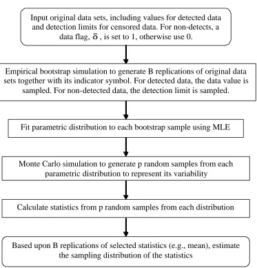
In the case of a censored data set, the conventional approach to parametric bootstrap simulation cannot be directly applied. Specifically, it is necessary to generate bootstrap samples so that there can be random variation in the number of data points that are below detection limit. If the data set is a single detection limit case, the data points below the detection limit can be determined as “censored”. However, in a multiple-detection- limit case, a detected point may have a value larger than a detection limit of a censored value if they come from different test facilities or testing methods. In order to deal with this issue, an empirical bootstrap approach is used. In empirical bootstrap simulation, each of the original n data points is sampled with

replacement and with equal probability of being sampled. In the original data set, either the value of data point is given for detected data or the detection limit is given for censored data.

Therefore, for each data point, an indicator symbol δ is given to indicate whether it is a detected value or below a detection limit. A value ofδequal to 1 was used to represent a data point below

(38)

4.0 Robustness Test of the Bootstrap Method for Quantifying Uncertainty

in the Statistics of Censored Data Sets

(39)

with multiple detection limits, 60 percent of the data set was assumed to be below one or more detection limits.

For cases with two detection limits, one detection limit was assigned to the 30 percent cumulative probability value, designated as DL2, and the other was assigned to the 60 percent cumulative probability value, designated as DL3. During bootstrap simulation, any randomly sampled value less than DL2 was treated as a non-detected value with a detection limit of DL2. Similarly, any sampled value greater than DL2 but less than DL3 was treated as a non-detected value with detection limit DL3. For cases with three detection limits, detection limits were assigned to the 10, 30 and 60 percentiles of the distribution, designated as DL1, DL2 and DL3, respectively.

For multiple detection limits as described above, non-detected values greater than one detection limit but less than another (e.g., between DL2 and DL3) were handled as interval-censored data.22 For example, for the lognormal distribution, the log- likelihood function for interval censoring with two detection limits is:

                  −     − +                   − + +         ₋ − − − =

∑

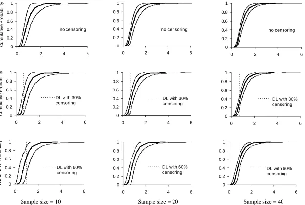
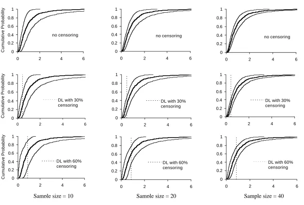
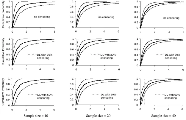
= 2 2 5 . 0 ln 2 1 5 . 0 ln 2 ) ( ) 2 ln( 2 ln ) , ( 1 2 2 1 1 1 2 2 σ σ µ σ µ σ µ π σ σ µ DL erf DL erf ND DL erf ND x n n J n i i (8)

(40)

The uncertainty in the cumulative distribution function of a specified parametric distribution is quantified based upon 95% confidence intervals obtained by bootstrap simulation. Figures 2 to 4 show uncertainty results for lognormal distributions with coefficients of variation of 0.5, 1 and 2, respectively. These figures show results for three sample size (10, 20 and 40) and for no censoring, 30% censoring and 60% censoring. Where applicable, the detection limit is shown by a vertical dashed line.

From Figure 2, the range of uncertainty becomes larger for the portion of the distribution below the detection limit as the percentage of censoring increases. Thus, as expected, there is more uncertainty regarding the estimate of the portion of the distribution that is below detection than there would be if all of the data had been detected. Comparing the three charts in any row of Figure 2, the 95% confidence interval of the specified distribution becomes narrower as the sample size increases from 10 to 20 to 40. Figures 3 and 4 reveals similar trends with respect to the amount of censoring and sample sizes. A comparison of Figures 2, 3 and 4 for the same percentage of censoring and the same sample sizes, reveals that the 95% confidence interval of the distribution gets wider as the coefficient of the variation increases from 0.5 to 1 to 2. Thus, the range of uncertainty is shown to increase as the range of variability increases with all else held constant. Although not shown, similar comparison were done for the gamma and Weibull distributions as a function of amount of censoring, sample size and coefficient of variation and similar results were obtained regarding the influence of the these factors on uncertainty.

(41)

(42)

When interpreted with respect to the confidence intervals of the mean, the deviations of the average mean values compared to the population mean values are small. For example, the mean of 1.13 for the lognormal case with n = 20, CV = 2, and 60% censoring has a 95 percent confidence interval of 0.48 to 2.49. The similar case for the Weibull distribution has a mean of 1.04 and a confidence interval of 0.38 to 2.22. Both confidence intervals well enclose the population mean of 1.00. As expected, for a given distribution, CV, and amount of censoring, the confidence intervals become narrower as the sample size increases. For a given sample size and CV, the confidence intervals tend to widen as the amount of censoring increases. However, the width of the confidence interval for any given distribution, sample size, and CV is relatively insensitive to the amount of censoring. As shown in Table 2, the detection limits for 30% and 60% censoring are typically less than or approximately equal to the mean value of the distribution. However, because means are more sensitive to large values than to small values, additional uncertainty in the non-detected region of the distribution does not substantially influence the confidence interval for the mean in this case. The only apparent exception to this trend is for the lognormal distribution with n = 20 and CV = 2, for which the upper bound of the 95 percent confidence interval changes with censoring. However, of all the cases considered these are numerically the least stable and the differences in results are only modest.

(43)

1.00 to 1.13. The highest average means occur for smaller sample size and fewer detection limits. A detailed investigation of the bootstrap samples revealed that the MLE method produces fitted distributions that are sensitive to sample values obtained in the upper tail. The sensitivity to such samples is greater for smaller sample sizes. Furthermore, the sensitivity to artifacts of samples from the upper tail are more influential for cases with only one detection limit versus cases with multiple detection limits. With multiple detection limits, more is known regarding the shape of the distribution in the non-detected region because the cumulative probability of each detection limit is included in the likelihood function. Thus, more constraint is imposed upon the shape of the distribution as the number of detection limits increases and, correspondingly, there is less influence of samples in the tail. Thus, although the MLE method is unbiased as sample size increases, for small sample values there can be apparent biases in the mean, especially for large CV and a tail- heavy parametric distribution. However, even in the worst case shown in Table 4, the 99 percent confidence interval of the mean well encloses the population values of 1.00.

(44)

other coefficients of variation and distribution types were also studied and similar results were obtained.

5.0 Evaluation of the Bootstrap Method for Estimating the Mean of

Censored Data Sets

The objective of this section is to verify that the MLE/Bootstrap method is reliable with respect to estimation of the mean even for small sample size. For this purpose, 20 synthetic data sets with sample size 20 were randomly generated from a gamma distribut ion with a mean of 1 and standard deviation of 1. The samples in the synthetic data set were ranked in ascending order. Different detection limits were assigned to each synthetic data set in order to achieve different amounts of censoring including 30% and 60%. That is, for each synthetic data, the detection limit corresponding to 30% censoring is assigned a value equal to the average of the 6th and 7th ranked data points in the 20 data points, and the detection limit corresponding to 60% censoring is assigned a value equal to the average of the 12th and 13th ranked data points. The MLE/Bootstrap method was applied to get the best estimate of the mean. The t-test was applied to the 20 best estimates of means to test if their average was statistically significantly different from the population mean of 1. The results are shown in Table 6.

For all three levels considered in Table 6, the p- values of the t test are larger than the significance level of 0.05. Therefore, the hypothesis can not be rejected which indicates that the best estimate of the means from the MLE/Bootstrap method are reliable for synthetic data sets.

(45)

The MLE/Bootstrap result of 0.990 is slightly different than the arithmetic average because MLE does not preserve the moments. However, the estimated mean is within one percent of the

population mean.

The methods of ignoring non-detected values and averaging only detected data, and of replacing non-detected values with the detection limit, are shown to overestimate the mean. The bias becomes more pronounced as the amount of censoring increases. Conversely, the method in which non-detected values are assigned a value of zero clearly underestimates the mean. The commonly used method of replacing non-detected values with one-half of the detection limit appears to be unbiased for the example of 30% censoring but the bias inherent in this method becomes obvious at 60% censoring. In the latter case, the population mean is overestimated by 6.5%. In contrast, the MLE/Bootstrap method provides consistent estimates of the mean

regardless of the amount of censoring. The maximum deviation of the estimated mean from the population mean in these three cases of censoring is only 1.4 percent. Although not shown in the paper, the same tests for lognormal and gamma distributions were also done and similar

conclusion can be drawn.

6.0 Verification of the Uncertainty Estimates from the Bootstrap Method

with the Kaplan-Meier Estimator Method

(46)

Meier estimator can be used in analyzing left-censored data sets.13 For this purpose, synthetic data sets with sample size of 40 were randomly generated from lognormal, gamma and Weibull distributions with mean equal to 1 and coefficients of variation equal to 0.5, 1 and 2. The samples in the randomly generated data set were ranked in ascending order. Different detection limits were assigned to the synthetic data sets in order to achieve 0%, 30% and 60% censoring. The MLE/Bootstrap method was applied to each synthetic data to get the CDF and the 95% confidence interval of the CDF.

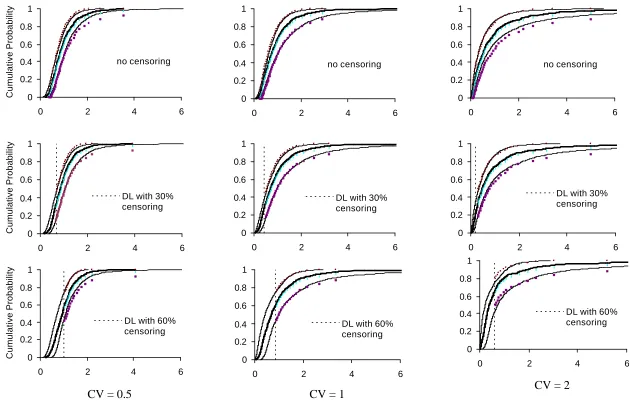
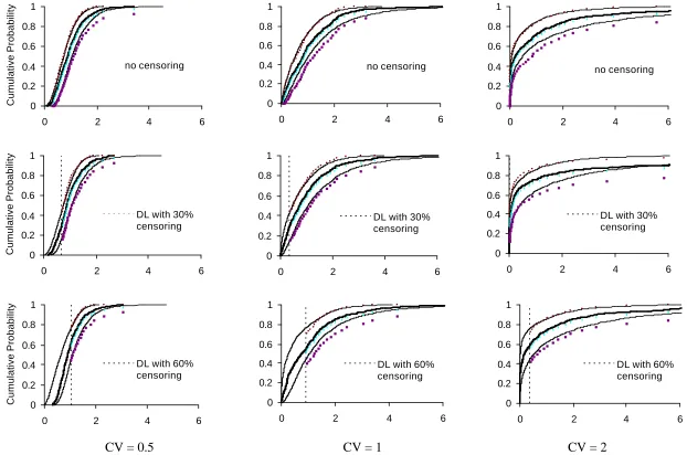
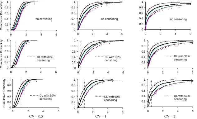
The test is to compare the 95% confidence interval of the CDF estimated by MLE/Bootstrap method and the Kaplan-Meier estimator. Since the Kaplan-Meier estimator method is a non-parametric method, 40 data points were evenly drawn from the CDF estimated by the MLE method and an empirical CDF and its 95% confidence interval were calculated for these 40 points using the Kaplan-Meier estimator method. Figures 5 to 7 show the comparison of the results of the confidence intervals of the CDF estimated from MLE/bootstrap and the Kaplan-Meier estimator methods for lognormal, gamma and Weibull distributions, respectively.

(47)

of the CDF from these two methods is only 2.7 percent for the lower level and 2.9 percent for the upper level. Similar inferences can be made in other cases shown in the figures.

7.0 Case Study for Estimation of Variability and Uncertainty in an

Emission Factor Based Upon Censored Data

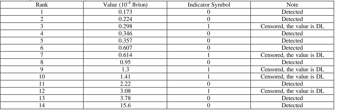
As an example of an emission factor data set that contains censoring, a data set for formaldehyde emissions from external combustion sources fired with bituminous and subbituminous coal combustion was selected. The data set is given in Table 8. The data set contains 14 data points, of which 5 are censored. Each of the five censored data points has a different detection limit. There are 2 data values that are greater than the largest of the five detection limits and 2 that are smaller than the smallest of the five detection limits. There are three detected data values that are greater than the smallest detection limit but smaller than the second smallest detection limit. There is one detected data value between the second and third detection limits. There is one detected data value between the fourth and fifth detection limits.

(48)

are larger. The uncertainty regarding the possible cumulative probabilities of the detected data points is indicated by solid vertical lines in Figure 8. For the 2 values that are larger than the largest detection limit, there is no uncertainty regarding the cumulative probability in these cases. The five detection limits are indicated by dashed vertical line.

From Figure 8, the fitted distribution agrees reasonably well with the observed data. The 95 percent confidence interval on the fitted distribution encloses all of the detected values. The graphical comparison of the data points and fitted distribution and its confidence intervals further confirm that lognormal distribution is a reasonable model to represent the inter-unit variability in the formaldehyde emission factors.

The detected formaldehyde emission factor data vary over almost two

orders-of-magnitude and the fitted distribution spans approximately three orders-of-orders-of-magnitude. Therefore, there is a large amount of uncertainty in the mean value associated with the small sample size, large amount of variability in the data, and the presence of non-detected measurements in the data set. The mean estimated based upon the fitted lognormal distribution was found to be 1.8 × 10-5 lb formaldehyde emitted per ton of coal combusted. The 95 percent confidence interval for the mean ranges from minus 77 percent to plus 209 percent of the mean value. The asymmetry of this confidence interval is based upon the large amount of variability in the data, the relatively small sample size, and the fact that an emission factor must be non- negative. The mean could be estimated from the conventional methods as well. The estimated means are 2.7 × 10-5, 1.7 × 10

-5_{, 2.0 ×}

(49)

the result based upon removing the non-detects, replacing non-detects with DL/2 or DL in this case.

8.0 Conclusions

(50)

The key advantages of the MLE/Bootstrap method is that it is a statistically rigorous, robust, and asymptotically unbiased method that can be used to make inferences for a wide variety of situations, including different types of distributions, coefficients of variation, sample sizes, and amounts of censoring with either single or multiple detection limits. Compared to simplified conventional methods, which are biased, the MLE/Bootstrap method is more computationally intensive. However, unlike conventional methods, the MLE/Bootstrap method enables estimation of uncertainty for any statistic, including the influence of uncertainty associated with censoring itself. The MLE/Bootstrap method can be incorporated as part of a two dimensional framework in which variability and uncertainty are distinguished. The MLE/Bootstrap method is recommended for consideration in environmental, risk assessment, and other policy relevant analyses in which censoring of data are present.

9.0 Acknowledgements

The authors acknowledge the support of the Science to Achieve Results (STAR) grants program of the U.S. Environmental Protection Agency, which funded this work under Grant No. R826790. Although the research described in this paper has been funded wholly or in part by the U.S. EPA, this paper has not been subject to any EPA review and therefore does not necessarily reflect the views of the Agency, and no official endorsement should be inferred.

10.0 References

(51)

Strategy, by EPA office of Air Quality Planning and Standards, 1999.

http://www.epa.gov/ttn/atw/urban/urbanpg.html (accessed by 10/1/ 2000) 2. Frey, H.C. and Rhodes, D.S. (1996) “Characterizing, Simulating, and Analyzing

Variability and Uncertainty: An Illustration of Methods Using an Air Toxics Emissions Example,” Human and Ecological Risk Assessment: an International Journal, 2(4): 762-797.

3. Frey, H.C., Bharvirkar, R., and Zheng, J. (1999) “Quantitative Analysis of Variability and Uncertainty in Emissions Estimation,” Prepared by North Carolina State University for Office of Air Quality Planning and Standards U.S. Environmental Protection Agency, Research Triangle Park, NC.

4. Frey, H.C. and Zheng, J., (2002) “Quantification of Variability and Uncertainty in Utility NOx Emission Inventories,” Journal of Air and Waste Management Association, 52(9):

1083-1096

5. Cullen, A.C. and Frey, H.C., (1999) Probabilistic Techniques in Exposure Assessment. Plenum Press: New York and London

6. Rao, S.T., Ku, J.Y., and Rao, K. S., (1991) “Analysis of Toxic Air Contaminant Data Containing Concentrations Below the Limit of Detection,” Journal of the Air and Waste Management Association, 41(4): 442-448

(52)

8. Newman, M.C., Dixon, P.M., Looney, B.B., and Pinder, J.E. (1989), “Estimating Mean and Variance for Environmental Samples with Below Detection Limit Observations,” Water Resources Bulletin, 25(4): 905-915

9. Haas, C.N. and Scheff, P.A. (1990), “Estimation of Averages in Truncated Samples,” Environmental Sciences and Technology, 24(6): 912-919

10. Elvira, B., Rao, S., and Porter, P.S. (1999), “Identifying Pollution Source Regions using Multiple Censored Data,” Environmental Sciences and Technology, 33(13): 2273-2277 11. Clarke, J.U. (1994), “Evaluating methods for statistical analysis of less than detection

limit data using simulated small samples. 2. General Results,” International Conference on Dredging and Dredged Material Placement, vol. 1: 747-755

12. Efron, B. and Tibshirani, R.J. (1993), An Introduction to the Bootstrap, Chapman & Hall: New York.

13. She, N. (1997), “Analyzing Censored Water Quality Data Using A Non-parametric Approach,” Journal of the American Water Resources Association, 33(3): 615-624. 14. Frey, H.C. and Bammi, S. (2002), “Quantification of Variability and Uncertainty in Lawn

and Garden Equipment NOx and Total Hydrocarbon Emission Factors,” Journal of the

Air & Waste Management Association, 52(4): 435-449

15. Seinfeld, J.H. (1986), Atmospheric Chemistry and Physics of Air Pollution, John Willey and Sons, New York

16. Casella, G. and Berger, R.L. (2001) Statistical Inference. Duxbury Press: Pacific Grove, CA.

(53)

18. Cohen, A.C. and Whitten, B. (1988), Parameter Estimation in Reliability and Life Span Models, M. Dekker: New York.

19. Frey, H.C. and Rhodes, D.S. (1998) “Characterization and simulation of uncertainty frequency distributions: Effects of Distribution Choice, Variability, Uncertainty, and Parameter Dependence,” Human and Ecological Risk Assessment, 4(2):423-468. 20. Press, W.H., Teukolsky, S.A., Vetterling, W.T., and Flannery, B.P. (1992). Numerical

Recipes in Fortran: The Art of Scientific Computing, 2nd ed., Cambridge University Press: New York.

21. Frey, H.C. and Zheng, J. (2002) “Technical Documentation of the AuvTool Software Tool for Analysis of Variability and Uncertainty,” Prepared by Department of Civil Engineering, North Carolina State University for Office of Research and Development, U.S. Environment Protection Agency, Research Triangle Park, NC.

(54)

Table 1. Parameters of the Assumed Lognormal, Gamma and Weibull Population Distributions with Coefficients of Variation of 0.5, 1 and 2

Distribution CVa Parameter1b Parameter2b

0.5 -0.112 0.472

1 -0.347 0.833

Lognormal

2 -0.804 1.269

0.5 4 0.25

1 1 1

Gamma

2 0.25 4

0.5 2.101 1.129

1 1 1

Weibull

2 0.543 0.575

a

Coefficient of Variation

b

Refer to equations (1), (2) and (3) for parameter definitions

Table 2. Detection Limits Associated with Different Cumulative Probabilities for Specified Population Distributions as a Function of Distribution Type and

Coefficient of Variation

Cumulative Probability for Detection Limit Distribution CVa

10% 30% 60%

0.5 0.488 0.698 1.008

1 0.243 0.457 0.873

Lognormal

2 0.088 0.230 0.617

0.5 0.436 0.691 1.044

1 0.105 0.357 0.916

Gamma

2 0.00027 0.022 0.377

0.5 0.387 0.691 1.083

1 0.105 0.357 0.916

Weibull

Probabilistic Modeling of Variability and Uncertainty in Urban Air Toxics Emissions

ABSTRACT

TABLE OF CONTENTS

LIST OF TABLES

LIST OF FIGURES

Part I

1.0

Introduction

Part II

QUANTIFICATION OF VARIABILITY AND UNCERTIANTY FOR

CENSORED DATA SETS AND APPLICATION TO AIR TOXIC

EMISSION FACTORS

Abstract. Many environmental data sets, such as for air toxic emission factors, contain several

1.0

Introduction

2.0

MLE Parameter Estimates for Censored Lognormal, Gamma and

Weibull Distributions

∑

∑

}

{

∑

∑

∫

(

)

∑

∑

3.0

Estimation Uncertainty in Statistics Using Bootstrap Simulation

4.0

Robustness Test of the Bootstrap Method for Quantifying Uncertainty

in the Statistics of Censored Data Sets

∑

5.0

Evaluation of the Bootstrap Method for Estimating the Mean of

Censored Data Sets

6.0

Verification of the Uncertainty Estimates from the Bootstrap Method

with the Kaplan-Meier Estimator Method

7.0

Case Study for Estimation of Variability and Uncertainty in an

Emission Factor Based Upon Censored Data

8.0

Conclusions

9.0

Acknowledgements

10.0 References