Application of Underwater Low Frequency Electromagnetic Fields
Detection with TSS FDTD Method
Kuisong Zheng*, Hui Yu, Huan Luo, and Tengjiang Ding
Abstract—Based on the conventional finite-difference time-domain (FDTD) method, a novel total-field scattered-total-field source FDTD method with a dual-meshed technique is presented to deal with the underwater detection problems in low frequency electromagnetic wave. A transformation surface connecting the coarse cell with the fine cell is implemented by applying a total-field scattered-field source (TSS) technique, which is carried out by two-step FDTD simulation. The ratio of a coarse cell size to a fine cell size can be set as an arbitrary integer, such as N = 10. Moreover, an analysis of numerical error illustrates that non-physical reflection fields from the TSS surface are avoided by introducing the TSS surface. We have derived, in detail, the update equations of fields on grids of the TSS surface. Three cases of dealing with different underwater electromagnetic problems are discussed. Numerical results show that by analyzing the magnitude and phase of scattered fields from obstacles underwater we can distinguish the category of the obstacles which belong to either a high resistivity body or a low resistivity body. Therefore, the proposed method provides us an effective tool for analyzing the electromagnetic response of materials underwater.
1. INTRODUCTION
The finite-difference time-domain (FDTD) method [1, 2] is arguably the simplest, both conceptually and in terms of implementation, of the full-wave techniques used to solve problems in electromagnetics. Recently, this method has turned out to be effective at extremely low frequency [3, 4]. The development of a reliable and accurate algorithm for underwater electromagnetic application has been a challenging problem for many years [3–5].
In underwater environment, the electromagnetic wave in the extremely low frequency range can propagate over long distance. The characteristics of underwater electromagnetic wave propagation imply that the computation domain needs to be meshed with a large cell size. However, in order to model the excited source more precisely, we need a fine cell size to mesh the space containing the excited source. For example, a loop antenna operating in low frequency is used to excite electromagnetic waves propagating in underwater. To overcome the contradiction, several subbgridding techniques have been reported in the literature [6–8]. However, the conventional subbgridding techniques have several disadvantages. The ratio of a coarse to fine cell size is usually less than or equal to 3, which is always not large enough to meet the requirement of underwater electromagnetic problem. Simultaneously, the exchange interface between the coarse cell and fine cell will lead to inevitable non-physical reflection.
In this paper, a novel dual-meshed technique is proposed. The basic idea of the method involves a two-step simulation procedure. These two simulations are connected by the establishment of a total-field scattered-field source (TSS) surface. In the first simulation, a fine cell size is employed. The radiated fields of an excited source on the TSS surface are stored for record. In the second simulation, the
Received 11 June 2014, Accepted 16 August 2014, Scheduled 8 September 2014 * Corresponding author: Kuisong Zheng ([email protected]).
equivalent currents are calculated with the recorded radiated fields, and then introduced into the range of total fields by the TSS surface. This method allows applying a large ratio of a coarse cell size to a fine cell size, such as the ratio N = 10. Furthermore, the introduced TSS surface does not affect the propagating of scattered fields from the obstacles. For stating conveniently, the proposed method is referred to as TSS FDTD method.
In the works [9–12], Huygens subgridding (HSG) method is presented to divide the entire problem space into several parts with different time and space increments. For the HSG, two spaces are connected by two Huygens surfaces called inner surface (IS) and outer surface (OS). The IS and OS are set close to each other, typically separated with 2 or 3 FDTD cells. For the proposed TSS FDTD method, the connected surface is established by only one FDTD cell of electric-field node or magnetic-field node. Moreover, for the proposed method, the ratio of a coarse cell size to a fine cell size can be set as an arbitrarily odd or even integer.
Certainly, the idea of dual simulation space to analyze the electromagnetic fields of extremely low frequency is first given in [13]. However, this reference does not state clearly how to obtain the accurate equivalent electromagnetic currents on the transformation surface. Moreover, in this reference, the authors only apply in either equivalent electric currents or equivalent magnetic currents to finish field transformation between these two simulation spaces. The above process will produce certain numerical errors. As we know, it is very important to carefully deal with the connection surface for the computation of dual simulation space. According to the reference, we extend the idea of the dual simulation space to present the TSS FDTD method. Using the TSS technique, we derive the iteration formulas of electromagnetic currents on the connection surface in detail.
The remainder of this paper is organized as follows. Section 2 introduce the two-dimensional TSS FDTD method. Section 3 illustrates the accuracy of the TSS FDTD method. Section 4 describes a complex case underwater to detect the obstacles with low frequency electromagnetic wave. Finally, concluding remarks are drawn in Section 5.
2. TSS FDTD METHOD
Ampere’s and Faraday’s laws are the relevant governing equations in constructing the FDTD algorithm. These equations are approximated by finite-differences at the appropriate points in space-time, yielding the discretized update equations. According to the Yee algorithm. For example, the update equation of Ez component in a two-dimensional case is
En+1
z (i, j) = CA(m)Ezn(i, j)
+CB(m)
Hn+1/2
y i+12, j
−Hn+1/2
y i−12, j
Δx −
Hn+1/2
x i, j+12
−Hn+1/2
x i, j−12,
Δy
(1)
The coefficients CA(m) and CB(m) in the update equation are assumed constant in time but may be functions of position. The detailed formulas of CA(m) and CB(m) can be referred to [1]. The equivalent source can be described as: the fields produced by an excited source located inside this part can be reproduced by impressing the following equivalent electric and magnetic current densities on the equivalent surface. These currents are therefore
Js=n×Hs Jms =Es×n (2)
wherenis the unit vector normal to the TSS surface. Es andHs are original tangential fields over the TSS surface.
As shown in Fig. 1, the TSS surface includes E-surface and H-surface. These two surfaces are adjacent to together. Usually, in FDTD we define the E-surface containing electric field nodes and
n
e
ms s
J = − ×n E
s s
J = ×n H
(a) (b)
CPML CPML
TSS surface
E-surface
H-surface Source
→ → →
→ → →
Figure 1. The problem spaces using in TSS FDTD method. (a) In the first simulation. (b) In the second simulation.
2 2
( )
z
E i
′ ′
δ
j
′
δ
2
0 2 2
( , )
2 y
H i′ ′δ +δ j′δ
1 0
( 1)
( , )
2
y
N
H i jδ δ+ − δ
0 1 1
z
E i
δ δ
j
10
( 1)
( , )
2
y
N
H + + δ
2/ 2 δ
y
x z
total field
E-surface
scattered field
H-surface
0
,
( )
,
1 1
i jδ δ1 1
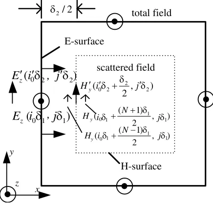
Figure 2. Diagram of nodes located on the TSS surface in TM mode.
the first simulation, the computation space, shown in Fig. 1(a), is meshed in a fine cell size in order to simulate the excited source precisely. In the second simulation the space is meshed in a coarse cell size in order to calculate radiated fields going through a long distance. Each computation space is surrounded by a convolution perfectly matched layer (CPML) absorbing boundary condition [14, 15] to model the open environment.
In a two-dimensional case, the TSS surface is an enclosed rectangular curve, illustrated in Fig. 2. For further conveniently stating the proposed method, we assume that the ratio of a coarse cell size to a fine cell size is set as N. The formula forN gives
δ2 δ1 =
Δt2
Δt1 =N (3)
whereδ1 and Δt1 are the spatial and time increments in the first simulation. Similarly,δ2 and Δt2 are the spatial and time increments in the second simulation.
The valueN takes on either an odd or even integer. We found that whenN is an even integer, the update equations of TSS FDTD are more complex than those whenN is an odd integer. Therefore, we emphasize how to implement the update equations whenN is an even integer.
currents on the TSS surface are obtained as
J−x
s =n×H =−x×(Hx, Hy,0) =−Hyz
J−x
ms =−n×E =x×(0,0, Ez) =−Ezy (4)
According to Fig. 2, assume that the variablesE and H with the symbol ‘’ are defined in the second simulation, and similarly, the variablesE and H without the symbol ‘’ are used in the first simulation. In Fig. 2, the arrow symbol ‘→’ stands for the nodes of magnetic field, and the circle symbol ‘•’ denotes the nodes of electric field. Seen from Fig. 2, the electric field node of Ez(i0δ2, jδ2) on the TSS surface belongs to the total-field zone. Referring to Equation (1), if we want to calculate the value of Ez(i0δ2, jδ2) on time instant (n+ 1)Δt, the update equation includes four magnetic field nodes. However, the node ofHy(i0δ2+δ2/2, jδ2) belongs to the scattered-field zone, and the other three nodes are located at the total-field zone. Therefore, in order to keep the same property of fields at both ends of equation, the update equation of Ez(i0δ2, jδ2) needs to introduce the incident fields at proper time instant and spatial position. According to the idea, the update equation of En+1
z (i0δ2, jδ2) can be
modified as
En+1
z i0δ2, jδ2= CA(m)Ezni0δ2, jδ2
+ CB(m)∇ ×Hnz+1/2 +CB(m)
4δ2 H
N(n+1/2)−1/2
y
i0δ1+ (N + 1)δ1 2 , jδ1
+HyN(n+1/2)+1/2
i0δ1+(N + 1)δ1 2 , jδ1
+HyN(n+1/2)−1/2
i0δ1+(N −1)δ1 2 , jδ1
+HyN(n+1/2)+1/2
i0δ1+(N−1)δ1 2 , jδ1
(5)
where the last four terms on the right-hand side of equation are the values of incident fields transformed from the radiated fields recorded in the first simulation. Note that in (5) the algorithm of central interpolation is used to introduce the incident fields at proper time instant and spatial position according to the previous fields recorded in the first simulation. As we all know, the algorithm of central interpolation has the second order accuracy. Meanwhile, the FDTD algorithm has also the second order accuracy. Therefore, according to the total-field scattered field technique, we can implement the field transformation at the TSS surface while maintaining the grid truncation errors within a proper acceptance.
In a similar manner, consider the H-surface parallel to y direction when x = (i0 + 1/2)δ1. Calculating the magnetic field node of Hy(i0δ2 + δ2/2, jδ2) in the scattered-field zone relates to
Ez(i0δ1, jδ1) in the total-field zone. So, the updated equation of Hyn+1/2(i0δ2 +δ2/2, jδ2) can be modified as
Hn+1/2
y
i0δ2+δ2 2, j
δ2 = CP(m)Hn−1/2
y
i0δ2+δ2 2, j
δ2
+CQ(m)∇ ×ENy + CQ(m)EzNn(i0δ1, jδ1)/δ2 (6) where the coefficients CP(m) and CQ(m) are functions of position analogous to coefficients CA(m) and CB(m). Note that the positions of nodes for the first and second simulations are related by
i0δ2 =i0δ1, jδ2 =jδ1 (7)
Similarly, the same processing is also taken for other nodes on the TSS surface. Limited space forbids further listing all update equations here.
3. VERIFICATION OF THE ACCURACY
3.1. Radiated Fields of Line Current
In this section, we verify the accuracy of the TSS FDTD method. Numerical results simulated by TSS FDTD are compared with the analytic solution and the conventional FDTD results.
Seen from Fig. 3, the calculation space is filled with a uniform water medium with εr = 80 and
(a) (b)
absorbing boundary
TSS surface
monitor line
A
4m
water water
source
x y
Figure 3. Diagrams of the problem space. (a) In the first simulation. (b) In the second simulation.
source is an electric dipole located atx=−0.5 m. The monitor point A away from the source is set as
lA = 1.0 m in the +x direction. The dashed-line rectangle presents the TSS surface with the physical dimensions 1.0 m×1.0 m. In the first simulation, the computation space with dimensions 1.1 m×1.1 m is meshed in a fine cell size, as shown in Fig. 3(a). With the help of the first simulation, we record the radiated fields of the excited source on the TSS surface. Then, the recorded fields are transformed as the equivalent electromagnetic currents which are used in the second simulation, in which the computation space with dimensions 4 m×4 m is meshed in a coarse cell size, as shown in Fig. 3(b).
The line current source with a Gaussian pulse type is defined as
I(t) = 10−10exp
−
t−T
T 2
T = 50 ns. (8)
Solving for radiation fields of a line current source polarized in the +zdirection, an analytic solution is given in [16]. Then, the formula for Ez component is given by
Ez(ρ, ω) = ˜k
2
4 IH
(2) 0
˜
kρ (9)
where H0(2) is the zeroth order of Hankel function of second kind, and ρ is the distance of the monitor point away from the line current source. The variable ˜kin (9) denotes the complex wave number.
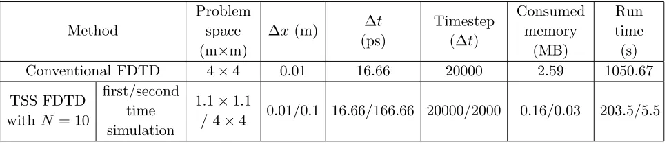
The related computation parameters are listed in Table 1 in detail. The computation environment is the PC HP Pro3380 CPU2.4 GHz MEM2.0 GB. The consumed memory and run time are also listed in Table 1. An inspection of Table 1 shows that the consumed run time in TSS FDTD is decreased to one-fifth of those spent by the conventional FDTD. In addition, the consumed memory is also greatly reduced in contrast to the conventional FDTD.
Table 1. Parameters used in the line current case.
Method
Problem space (m×m)
Δx(m) Δt (ps)
Timestep (Δt)
Consumed memory
(MB)
Run time (s) Conventional FDTD 4×4 0.01 16.66 20000 2.59 1050.67 TSS FDTD
with N = 10
first/second time simulation
1.1×1.1
/ 4×4 0.01/0.1 16.66/166.66 20000/2000 0.16/0.03 203.5/5.5
0 50 100 150 200 250 300 -3
-2 -1 0 1 2 3 4
Ez
/(V/m)
t/ns
Conventional FDTD TSS FDTD with N=10
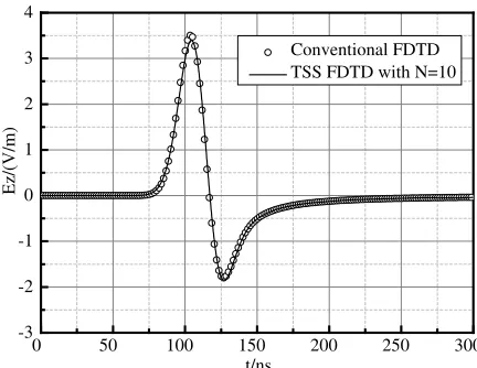
Figure 4. Radiation fields of a line current at the monitor point A.
0.0 0.4 0.8 1.2 1.6 2.0 2.4
0 2 4 6 8 10
Ez
/(mV/m)
Distance/m
Analytical solution Coventional FDTD TSS FDTD with N=10
0.5 1.0 1.5 2.0 2.5
0.00 0.05 0.10 0.15 0.20 0.25 0.30
Er
ror (m
V
/m
)
The conventional FDTD method The TSS FDTD method
(a) (b)
Distance/m
Figure 5. Amplitude distributions of Ez fields. (a) In the operating frequency f = 1 kHz. (b) The errors of these two methods.
the conventional FDTD simulation, and the solid line represents the results of TSS FDTD withN = 10. It is noted that the radiated fields in TSS FDTD are in well agreement with those in the conventional FDTD method.
Figure 5(a) represents the amplitude distributions ofEzcomponent along thexaxis in the working frequency f = 1 kHz. The horizontal coordinate axis represents the distance away from the source in thexaxis, and the vertical coordinate axis shows amplitudes of theEz field. The discrete star ‘*’ stands for the results with the conventional FDTD. Similarly, the circle ‘o’ represents the results simulated by the TSS FDTD with N = 10. For comparison, the analytic solution is also plotted in Fig. 5(a), marked by the solid line. By comparing these curves in Fig. 5(a), we find that the simulated results are in well agreement with analytic solution. In particular, the ratio of cell size in TSS FDTD to that in the conventional FDTD is set as N = 10. Seen from Fig. 5(a), zero values appear in the range of (0, 0.4 m) according to the TSS FDTD simulation, which imply no fields propagating inside the TSS surface, which means that in the second simulation of TSS FDTD the radiated fields only propagate out of the TSS surface and no incident fields inside of the TSS surface.
Figure 5(b) gives the absolute error distributions of these two methods at the monitor line. The error formula which we used is
which is the difference between the simulated results and the analytic solution. An inspection of Fig. 5(b) shows that at the range of interest, the absolute error of TSS FDTD withN = 10 is less than that of the conventional FDTD. The maximum absolute error of TSS FDTD withN = 10 is about 0.20 mV/m, which is within proper acceptance. An analysis of the error shows that the TSS FDTD method can reduce the run time and consumed memory while maintaining the absolute error within acceptance range.
3.2. Verifying the Scattered Fields
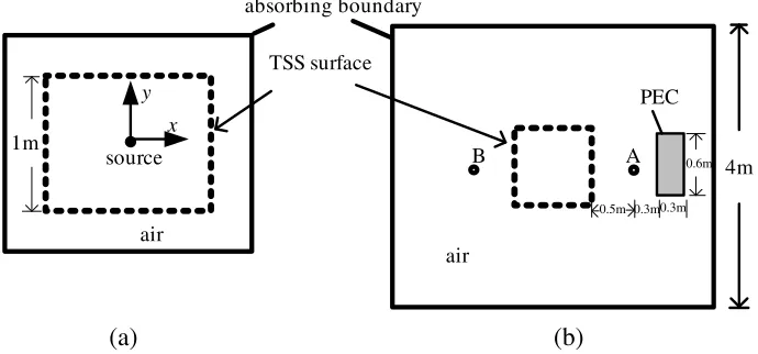
Another typical case with scattered object located in the problem space is discussed. The goal is to prove that the establishment of a suitable TSS surface has no impact on the propagation of scattered fields. In Fig. 6 the calculation space is filled with a uniform air medium withεr= 1.0 andσ = 0 S/m. A perfect electric conductor (PEC) slab with dimensions 0.6 m×0.3 m is symmetrically placed in thex axis, as sketched in Fig. 6. The PEC slab is located away from the source with the distance l= 1.3 m along the +x direction. The source is a line current with a Gaussian type waveform located at the center of the computation space. The monitor points A and B are symmetrically placed in the x axis. The distance between each monitor point and the origin is set as 1 m. In Fig. 6, the dashed-line square presents the TSS surface with the length 1.0 m. In this case, we use the TSS FDTD with N = 10 to calculate scattered fields caused by the PEC slab.
source
TSS surface
air air
absorbing boundary
0.6m
0.3m 0.5m
PEC
A
x y
0.3m
1m
4m B
(a) (b)
Figure 6. Diagrams of the calculation space of TSS FDTD. (a) In the first simulation. (b) In the second simulation.
The related computation parameters in TSS FDTD are listed in Table 2. In order to verify the results with TSS FDTD, and we also use the conventional FDTD to deal with the same case.
Table 2. Computation parameters in the case.
Method Problem space (m ×m) Timestep (Δt) Δx (m) Δt(ps)
Conventional FDTD 4×4 12000 0.01 16.6
TSS FDTD withN = 10
first/second
0 10 20 30 40 -60
-40 -20 0 20 40 60
Ez
/(V/m)
t/ns
Conventional FDTD TSS FDTD with N=10
0 10 20 30 40
-50 -25 0 25 50 75
Ez
/(V/m)
t/ns
Conventional FDTD TSS FDTD with N=10
0 10 20 30 40
-1.5 -1.0 -0.5 0.0 0.5 1.0 1.5
Er
ro
r(
V
/m
)
t/ns
Error at A Error at B
(a) (b)
(c)
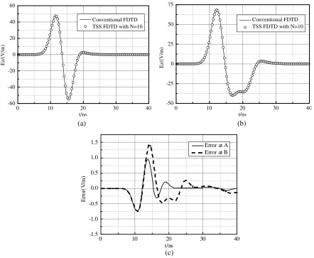
Figure 7. Comparison of the results of these two methods. (a) Point A. (b) Point B. (c) The errors.
electromagnetic fields between these two simulations with the central interpolation technique. The second-order accurate method of central interpolation will cause a little error into the numerical results. Nevertheless, from Fig. 7(c), the maximum absolute error of point B is equal to 1.4 V/m occurring on
t= 14.2 ns, which is to say that the maximum relative error of point B is equal to 2%, within proper acceptance. The absolute error of point A is less than that of point B at each time instant.
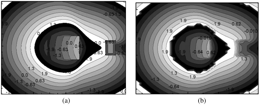
In order to graphically display how scattered fields propagate through the TSS surface, phase snapshots are recorded and drawn in Fig. 8. The recorded time instant is t = 26.66 ns, and the operating frequency is f = 200 MHz. Seen from Fig. 8, the phase distributions inside of TSS surface satisfy the characteristic of a propagating wave of scattered fields, which means that the scattered fields go through the TSS surface and spread without non-physical reflection caused by the existence of TSS surface. An inspection of Figs. 8(a) and (b) shows that the phase snapshots obtained by TSS FDTD are consistent with those by the conventional FDTD. Therefore, this example also verifies the validity of the TSS surface in TSS FDTD.
In summary, an analysis of these two cases verifies that the TSS surface is valid and available to simulate the original excited source.
4. DISTINGUISHING OBSTACLES UNDERWATER
(a) (b)
Figure 8. The phase snapshots ofEz-field in thexoy plane. (a) The conventional FDTD. (b) The TSS FDTD withN = 10.
source
observation points
200m air
400m water
underwater ground obstacle A
20m
700m
y
x TSS surface
obstacle B
700m
0
20m
Figure 9. The geometry model of the example.
Table 3. Properties of the materials in the example.
Material εr σ (S/m)
air 1 0
water 80 0.018
underwater ground 6 0.33 high resistivity body 1 0
low resistivity body 4 100
Table 4. Three cases in the example.
@
@@ obstacle A obstacle B
Case 1 underwater ground
underwater ground
Case 2 high resistivity body
low resistivity body
Case 3 low resistivity body
high resistivity body
There are two obstacles within the range of underwater ground. In order to keep unit consistence with the previous cases, we still use the International System of units in this section. The water layer is 400 m thick. The sizes of these two obstacles are the same as 200 m×700 m. For the TSS FDTD method with
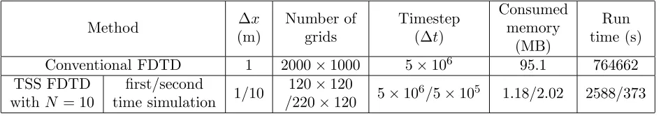
Table 5. Comparison of these two methods.
Method Δx
(m)
Number of grids
Timestep (Δt)
Consumed memory
(MB)
Run time (s)
Conventional FDTD 1 2000×1000 5×10⁶ 95.1 764662 TSS FDTD
with N = 10
first/second
time simulation 1/10
120×120
/220×120 5×10
6/5×105 1.18/2.02 2588/373
The excited source is a line current source with a Gaussian pulse type placed in water with the distancey= 200 m from the most upper interface. Establish the Cartesian coordinate system, as shown in Fig. 9. The source position is assumed to set as the origin of system. There are total 12 observation points to be recorded, marked by integer numbers from 1 to 12. These observation points are linearly equally distributed with the spacial increment Δx = 100 m along the x axis. The first point is set as the location with the distancey=−180 m directly below the excited source. The distance between the plane containing these observation points and the upper surface of obstacles is 40 m. The observation points 1 to 4 are located above obstacle A, and observation points 5 to 12 are above obstacle B.
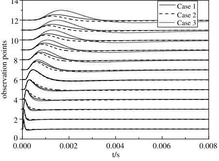
Due to the dispersion characteristics of water and ground, it takes millions of time-steps to record the entire pulse at these observation points. Table 5 lists many parameters used in these two methods. An inspection of Table 5 shows that it takes almost 764662 seconds to deal with the case, if we use the conventional FDTD method, which is unacceptable. If we use the proposed method, however, only 2961 seconds for the two-step simulation are required to calculate the same case. The run time in TSS FDTD is 0.4% less than that in the conventional FDTD. Therefore, comparing the conventional FDTD method, a lot of run time and consumed memory are greatly saved by using TSS FDTD with N = 10. Figure 10 shows the normalized waveform recorded at the 12 observation points. Seen from Fig. 10, it is noted that different constitutive parameters cause different waveforms at each observation point. In Fig. 10, the solid line denotes field distributions versus time at observation points when there are no obstacles inside of the underwater ground, as marked by Case 1. The dashed line stands for field distributions versus time when obstacle A and obstacle B are designated as the high resistivity body and low resistivity body, respectively, as marked by Case 2. The dotted line is the case when obstacle A and obstacle B are assigned as the low resistivity body and high resistivity body, respectively, as marked by Case 3. By comparing these curves for different cases, it is known that field intensities for observation points 1 to 4 in Case 2 are stronger than those in Case 3. This is the reason that in Case 2 there is a high resistivity body below observation points 1 to 4, but a low resistivity body in Case 3 below these observation points. On the contrary, for observation points 7 to 12, field intensities in Case 3 are stronger than those in Case 2. It is the reason that below observation points 7 to 12, there is a high resistivity body in Case 3, but a low resistivity body in Case 2. Due to radiated fields obliquely propagating through observation points 5 and 6, the field intensity differences are gradually diminished. Therefore, we can clearly distinguish types of obstacle underwater by analyzing the characteristic of field intensity.
In order to further clearly express characteristics of scattered fields from different types of obstacles, we consider the difference of field intensities between Case 2 or Case 3 and in Case 1. As shown in Fig. 11 in detail, the dashed line represents the difference of field intensity between Case 2 and Case 1, and the solid line stands for the difference between Case 3 and Case 1. By analyzing these two curves in Fig. 11, it is found that the sign of difference is reversed from observation points 1 to 12. Moreover, for observation points 1 to 5 the differences marked in solid line take on the minus sign in the first peak, while the difference in dashed line is the positive sign in the first peak. Similarly, for observation points 7 to 12 the difference in solid line takes on the positive sign in the first peak, while the difference in dashed line is the minus sign. The reason for the special phenomenon is that the obstacles in Case 3 are aligned in a proper order with the low resistivity body and the high resistivity body along the x axis, while Case 2 are the high resistivity body and the low resistivity body along the x axis.
0.000 0.002 0.004 0.006 0.008 0
2 4 6 8 10 12 14
observation points
t/s
Case 1 Case 2 Case 3
Figure 10. Normalized waveform at the
observation points.
0.000 0.002 0.004 0.006 0.008
0 2 4 6 8 10 12
-+ + + + + +
+ + + + +
observation points
t/s
Case 3-Case 1 Case 2-Case 1
+
Figure 11. Normalized amplitude differences at the observation points.
that for observation points 1 to 5 the phase in Case 3 of phase lags compared with that in Case 2. On the contrary, the phase in Case 3 for observation points 7 to 12 are of phase advance compared with that in Case 2, which means that the waveform of scattered fields in Case 2 first propagates through observation points 1 to 5 compared with that in Case 3. On the contrary, the waveform in Case 3 first propagates through observation points 7 to 12 compared with that in Case 2. It is the reason that the alignment of obstacles A and B is in a different order within underwater ground. The phase difference of scattered fields between Case 2 and Case 3 implyies that the velocity of propagating wave is different through different media. Fig. 10 and Fig. 11 show that the propagating velocity in high resistivity body is faster than that in low resistivity body. This conclusion is consistent with the rule of electromagnetic wave propagation [16].
5. CONCLUSION
A two-dimensional TSS FDTD method has been proposed for detecting obstacles underwater with low frequency electromagnetic wave in this paper. With the dual discretization technology, the TSS FDTD method includes a two-step procedure to simulate the electromagnetic field problems. The space including the excited source is meshed in a fine cell size. The remaining space including the obstacles is meshed in a coarse cell size. The spatial increment ratio of a coarse cell size to a fine cell size can be set as an arbitrary integer, such as N = 10. These two simulations are related by the TSS surface. We verify the validity of the TSS FDTD by two cases. One case is to simulate the radiated fields of line current source. The other is to show the scattered fields from obstacles can properly propagate through the connecting TSS surface. An analysis of the absolute error shows that the establishment of TSS surface is valid and suitable. Finally, a case of detecting obstacles within underwater ground is presented. Numerical results show that by analyzing the magnitude and phase of scattered fields from obstacles underwater, we can distinguish the category of the obstacles which is either a high resistivity body or a low resistivity body. For the low resistivity body, it may be a kind of metal underwater, and the high resistivity body probably is a kind of oil-gas underwater. For example, we can use the proposed method to analyze scattered fields underwater for distinguishing the oil-gas resource from the metal obstacles. Therefore, the proposed method provides us an effective tool for analyzing the electromagnetic response of materials underwater.
ACKNOWLEDGMENT
REFERENCES
1. Allen, T., Computational Electrodynamics: The Finite-difference Time-domain Method, 2nd Edition, Boston, 2000.
2. Yee, K., “Numerical solution of initial boundary value problems involving maxwell’s equations in isotropic media,”IEEE Transactions Antennas and Propagation, Vol. 14, 6–10, 1966.
3. Xia, Y. and D. M. Sullivan, “Underwater FDTD simulation at extremely low frequencies,” IEEE Antennas and Wireless Propagation Letters, Vol. 7, 661–664, 2008.
4. Furse, C. M., “Faster than Fourier: Ultra-efficient time-to-frequency-domain conversions for FDTD simulations,” IEEE Antennas and Propagation Magazine, Vol. 42, 24–34, 2000.
5. Loach, P. D., J. J. Kazik, and R. C. Ireland, “Numerical modelling of underwater electromagnetic propagation,” Recent Advances in Applied and Theoretical Mathematics, 220–225, 2000.
6. Chen, J. and A. Zhang, “A subgridding scheme based on the FDTD method and HIE-FDTD method,”Applied Computational Electromagnetics Society Journal, Vol. 26, No. 1, 1–7, 2011. 7. Yu, W. and R. Mittra, “New subgridding method for the finite-difference time-domain (FDTD)
algorithm,”Microwave and Optical Technology Letters, Vol. 21, No. 5, 330–333, 1999.
8. Mock, A., “Subgridding scheme for FDTD in cylindrical coordinates,” PIERS Proceedings, 1053– 1057, Suzhou, China, Sep. 12–16, 2011.
9. Berenger, J. P., “A Huygens subgridding for the FDTD method,”IEEE Transactions on Antennas and Propagation, Vol. 54, No. 12, 3797–3804, 2006.
10. Berenger, J. P., “Extension of the FDTD huygens subgridding algorithm to two dimensions,”IEEE Transactions on Antennas and Propagation, Vol. 57, No. 12, 3860–3867, 2009.
11. Berenger, J. P., “The Huygens subgridding for the numerical solution of the Maxwell equations,” Journal of Computational Physics, Vol. 230, No. 14, 5635–5659, 2011.
12. Abalenkovs, M., “Huygens subgridding for 3-D frequency-dependent finite-difference time-domain method,”IEEE Transactions on Antennas and Propagation, Vol. 60, No. 9, 4336–4344, 2012. 13. Xia, Y. and D. M. Sullivan, “Dual problem space FDTD simulation for underwater ELF
applications,” IEEE Antennas and Wireless Propagation Letters, Vol. 8, 498–501, 2009.
14. Sullivan, D. M. and Y. Xia, “A perfectly matched layer for lossy media at extremely low frequencies,”2009 IEEE International Symposium on Antennas and Propagation and USNC/URSI National Radio Science Meeting, Institute of Electrical and Electronics Engineers Inc., North Charleston, SC, United States, Jun. 1–5, 2009.
15. Roden, J. A. and S. D. Gedney, “Convolution PML (CPML): An efficient FDTD implementation of the CFS-PML for arbitrary media,” Microwave and Optical Technology Letters, Vol. 27, No. 5, 334–339, 2000.