Multi-Look SAR ATR Using Two-Level Decision Fusion of Neural
Network and Sparse Representation
Xuan Li, Chunsheng Li, and Pengbo Wang*
Abstract—As for the lack of the contribution by decision fusion in pose estimation and the demand for the combination of the feature fusion and the decision fusion in SAR ATR, in this paper, with the help of pose estimation, a new multi-look SAR ATR method is proposed in order to improve the performance, which is based on two-level decision fusion of neural network and sparse representation. The first-level decision fusion is acted for the combination of the pose estimation result by neural network and sparse representation. Based on the constraint of pose, these two models are exerted for the multi-look SAR ATR, and the second-level decision fusion is used to achieve the final recognition result. Several experiments based on MSTAR are conducted, and experimental results show that our method can achieve an acceptable result.
1. INTRODUCTION
As an active microwave sensor, Synthetic Aperture Radar (SAR) can observe the target all-time and overcome the constraint of weather and illumination. Thus, the Automatic Target Recognition (ATR) based on SAR image plays a crucial role in the real-world applications, such as military reconnaissance, geographic information interpretation, and disaster estimation. Compared with the optical image, the strong multiplicative speckle noise and vulnerability to the interference of outer conditions pose great difficulty on SAR ATR.
SAR images are highly sensitive to the target aspect [1, 2]. Therefore, the exploitation of multiple looks of the same target from different aspect angles may boost the performance than only using a single look [2]. In addition, the classifier fusion strategy is an effective way to improve the recognition rate [3], and it has been adopted in SAR ATR [4, 5]. Thus, the information fusion is a key point in SAR ATR, which mainly lies on two aspects: feature fusion and decision fusion. For feature fusion, a multi-look averaging scheme is proposed [6]. HMM has been utilized to model features of multi-look SAR images [7, 8]. The Joint Spares Representation (JSR) method has also been developed to bind results of different looks in order to exploit the interrelation [9]. For decision fusion, Bayes rule has been widely applied in SAR ATR [10]. The method of combining results from sparse representation and SVM by the Bayes rule is exerted to improve recognition rate [4]. SVM, KNN and MINACE are used to classify the feature of EFDs, PCA and 2D-DFT respectively. Then, D-S theory of evidence is exerted to fuse results of the three classifiers [5]. The hypothesis-level fusion by finding the optimal template that matches the whole looks has been introduced [11]. Other fusion strategies, such as PCA based data fusion [12], ranking based decision fusion [13] are also been evaluated.
Apart from that, another way to improve the performance is to add constraint on the input data. The most common one is on aspect angle constraint, which can improve the recognition rate to some extent [14]. In this sense, the acquirement of the target’s aspect angle by pose estimation is vital for recognition. Nowadays, techniques for pose estimation can be classified into two classes [15]: One
Received 23 September 2015, Accepted 17 December 2015, Scheduled 27 January 2016 * Corresponding author: Pengbo Wang ([email protected]).
achieves its goals by extracting some information on orientation of the target. Four criteria on target-to-background ratio are defined [16], which are perimeter, edge, pixel-count and hough transform, to find the aspect angle. A fast approximation to the 2-D CWT to provide precise target orientation information has been suggested [15]. A pose estimation method via edge detection is adopted [17], and the other trains a classifier by images with known aspect angle to predict the pose. For example, Principe et al. develop a training method on neural network for angle prediction [18].
Aiming at combining advantages of pose estimation, feature fusion and decision fusion, we propose a new method of multi-look SAR ATR using two-level decision fusion of Neural Network (NN) and Sparse Representation (SR) in this paper. Firstly, NN and SR are exerted for pose estimation respectively, and their results are combined via the first-level decision fusion. With the combined result of aspect angle, these two models are also used for classification. The second-level decision fusion is utilized to make the final recognition result. Here, the decision fusion method is exploited twice. One is in the combination of pose result, and the other is in the combination of recognition rate. The experimental result shows that there is an obvious improvement of recognition rate compared with other methods.
The rest of the paper is organized as follow. Section 2 illustrates the basic information of NN and its use in SAR ATR. It also introduces the SR and JSR for multi-look SAR ATR. Section 3 mainly focuses on the two-level decision fusion method. Section 4 shows the experimental setup and results. Then Section 5 gives the conclusion of this work.
2. SAR ATR BASED ON NEURAL NETWORK AND SPARSE REPRESENTATION 2.1. Neural Network
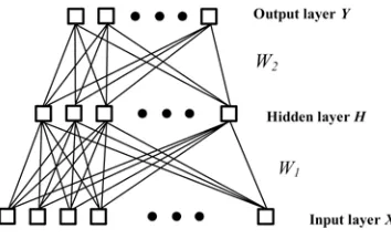
Since the NN has an advantage on the fitting of non-linear function, NN has been widely used in SAR ATR [19]. Fig. 1 shows a typical three-layer NN structure.
Figure 1. Architecture of neural network.
In Fig. 1, X is the input layer, H the hidden layer, representing the intermediate result of the NN, and Y the output layer. When training a NN, the input data should contain two parts: one is the input feature, whose dimension is the same as the input layer; the other is the ideal output, which constructs the label for the training. Loss function is essential for the training of NN, which measures the difference between the practical output (the value of the output layer) and the ideal output (the label). It is common to adopt the gradient descent (GD) to optimize the NN. The derivate of the loss function with respect to parameters of NN will be used in GD.
θnew=θ−α∂J(θ)
∂θ (1)
In Eq. (1), J(θ) is the loss function, θ the parameter of NN, and α the learn rate. Through the iterated utilization of Eq. (1), the value of the loss function will decrease, and the network will reach the global optima if the loss function is the convex function. Although it sometimes may not be convex, this method works fairly well in real-world application [21]. Other optimization algorithms, such as CG, Hessian-free, BFGS, can also be exerted to train the NN.
high accuracy [18]. However, it also brings some disadvantages when applied in practical situation: Firstly, non-parameter learning strategy is adopted in this method, indicating that large number of training samples must be stored to calculate the loss function, which will cost considerable memory. Moreover, the Havrda-Charvat entropy is used to build the loss function, whose calculation is O(N2), indicating a great burden on its practical use, especially when the amount of training data is large since it is necessary for the improvement of recognition rate. The performance of this method is tested as “PE by MI” in 4.3.
2.2. Sparse Representation
Suppose a dictionary matrix D, whose every column is the normalization result of training data, and the training data belonging to the same class are arranged together. On the other hand, the test sample y can be considered as the result of the linear combination of training samples:
y=x1d1+x2d2+· · ·+xNdN+ (2)
In Eq. (2), d1, d2, . . . , dN are normalization results of training data, x1, x2, . . . , xN the sparse coefficients, andis the residual error. Meanwhile, Eq. (2) can be changed into the following form:
y=Dx+ (3)
Here,D= [d1, d2, . . . , dN] andx= [x1, x2, . . . xN]T. For the sparse representation, the dictionaryD should be over-complete, which means the number of training samples is larger than its dim. Thus, in order to recover the optimal sparse representation ˆx, the sparse inducing norm, such asl1-norm, will be introduced. It meets the following requirements.
ˆ
x= arg min
x y−Dx 2 2
s.t.x1 ≤K (4)
K is the sparse level in (4). The optimal sparse representation ˆx can be induced by MP, OMP and some other methods. For the classification, the class of the test sample will be figured out by Eq. (5)
ˆi= arg min
i y−Dδ i(ˆx)
2 (5)
In Eq. (5),δi(ˆx) means that units in ˆx, corresponding to the training data of the classiin D, are reserved, while other units are set to 0. In this way, the class of the test sampley is defined as the one that can reach the minimal reconstruction error with respect to certain sparse level.
In order to boost performance, a strategy to introduce the target’s pose in SR is provided in [20], in which the test sample is represented by the training data with similar aspect angles. According to the analysis in [20], the disturbance of some highly-correlated samples attached to other classes can be removed and an obvious improvement of recognition rate will be witnessed in this way.
In terms of the multi-look SAR ATR, the JSR method is proposed in [9]. Here, test data with consecutive aspect angles are jointed into a matrixY = [y1, y2, . . . , ym], wheremis the number of looks, to replace they in Eq. (4). Apart from that, new requirement for the sparse representation ˆX is defined as follow:
ˆ
X= arg min
X Y −DX
2 F
s.t.Xl0\l2 ≤K (6)
Here,X is composed by the sparse representation of y1, y2, . . . , ym. Xl0\l2 means the mix-norm
of X obtained by first applying l2-norm on its every row and thenl0-norm are exerted on the result.
3. MULTI-LOOK SAR ATR VIA TWO-LEVEL DECISION FUSION
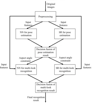
Figure 2. Method frameworks.
fusion. For the pose estimation, a new method based on decision fusion is also proposed in this paper. Here, we choose NN and SR as basic classifiers since they have been widely used in multi-look SAR ATR and achieve high performance.
The frame of our method is showed in Fig. 2. Firstly, NN and SR are exerted for the pose estimation based on features extracted by the preprocessing. The first-level decision fusion is acted to combine their results in order to improve the accuracy of the aspect angle prediction. Then, NN and JSR are used for the multi-look SAR ATR with the help of pose estimation results. Finally, the second-level decision fusion is applied to acquire the final recognition result.
3.1. Neural Network for the Pose Estimation
In our method, the non-parametric learning strategy in [18] is modified to the parametric learning. The data are classified into several categories, each one corresponds to a certain range of aspect angle with the same length. For example, when the length of the range is set toδ , data whose angles fall in [0, δ] are in class 1 and the data of [δ,2δ] are in class 2, and so on. Every unit in the output layer is related to one class. In this way, the continuous aspect angle of input image is discretized into several classes making the problem become a multi-class one. Since the soft-max regression is a common multi-class classifier [22]. It is adopted for the training of last layer in NN and the loss function of NN is replaced by the cross entropy, that is:
J(θ) =− C
i=1
lilogpi (7)
output layer, meaning the conditional probability pi =p(ci|s), where s is the input and ci the classi. C is the number of classes. The derivation of this equation is as follows:
∂J(θ)
∂oi =pi−li (8)
Here,oi in the equation is the activation of the unitiin output layer. It can be concluded that the calculations of Eqs. (7) and (8) are tremendously less than the Havrda-Charvat entropy in [18].
However, if the common label structure is adopted to define labels, which contain only 0 and 1, labels of the data that lie on the boundary of adjacent classes will fail to represent aspect angles of the data in the process of discretization. For example, suppose the class i and class i+ 1 correspond to the aspect angle range of [δi, δi+δ] and [δi+δ, δi+ 2δ], training sample s1 and s2 with aspect angle of δi + 0.5δ and δi+δ−, where is a small variable, will own the same label via the common label structure. Obviously, this label doesn’t have the ability to show the different positions of s1 and s2. Moreover,s2 is relatively near the class i+ 1. But the unit corresponding to class i+ 1 in its label is 0, which is the same as some data that may be far from the classi+ 1. Thus, the common label structure cannot reflect the data’s position, especially for the data near the boundary. To attain this goal, label l is changed as follows:
l =
0,0,· · ·, ti+1 ti+ti+1,
ti
ti+ti+1,· · ·, 0
1×C
ti = |a−ai|, ti+1 =|a−ai+1| (9)
In Eq. (9),ameans the aspect angle of the sample, andai and ai+1 are centers of the aspect angle range of class i and i+ 1, which refer to δi + 0.5δ and δi + 1.5δ. For the new label l, only the two nearest classes are considered. Because even if we take other classes into account, their corresponding unit values are relatively small, which will not pose obvious effects on the training of NN.
3.2. Sparse Representation for the Pose Estimation
The process of SR can be explained as the transformation of the test data to the space defined by the training data. The correlation coefficient of training sample di to the test sample y can be calculated asy, di.
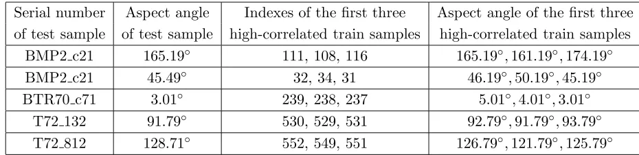
Table 1. Information of the first three highly-correlated train samples.
Serial number Aspect angle Indexes of the first three Aspect angle of the first three of test sample of test sample high-correlated train samples high-correlated train samples
BMP2 c21 165.19◦ 111, 108, 116 165.19◦,161.19◦,174.19◦ BMP2 c21 45.49◦ 32, 34, 31 46.19◦,50.19◦,45.19◦ BTR70 c71 3.01◦ 239, 238, 237 5.01◦,4.01◦,3.01◦
T72 132 91.79◦ 530, 529, 531 92.79◦,91.79◦,93.79◦ T72 812 128.71◦ 552, 549, 551 126.79◦,121.79◦,125.79◦
From Table 1, it can be discovered that some highly-correlated training samples’ aspect angles are close to the test sample. Thus, these high-correlated samples have the potential to estimate the aspect angle. Details about the experiment of Table 1 can be found in 4.1.
So, we can try to achieve pose estimation by SR with the following steps: Firstly, according to the correlation coefficient, for the test sampley, the firstktraining data in the dictionary are chosen. Then, these data are classified according to their aspect angles by the way of discretization in 3.1. Suppose the data classified to the class iared(1i), d
(i) 2 , . . . , d
(i)
n , which can be combined to the matrix D(i). Thus y will be represented by (10).
In Eq. (10), w is the coefficient and e the error. Here, Eq. (10) can be treated as the linear regression, and Normal equation will be used to getw which is able to minimizee. The class with the lowest error is regarded as the result of the test sample.
w= (D(i)TD(i))−1D(i)Ty (11)
The method of sparse representation for the pose estimation is performed as follows:
1. Calculate the correlation coefficient between the test sample and every train sample in the dictionary.
2. Choose some training data which have the first largest correlation coefficients.
3. Combine these chosen training data into several sub-dictionary D(i) according to their aspect angles. The training data belonging to the same angle class are combined into the same dictionary.
4. Reconstruct the test sample by Eq. (11). The test sample belongs to the angle class, whose sub-dictionary has the least reconstruction error.
3.3. Decision Fusion for the Pose Estimation
From 3.1 and 3.2, it can be concluded that the output of the pose estimation by NN, P ENN = [p1, p2, . . . , pC], is the probability that the input belongs to each class. On the other hand, the result of SR is just the most likely class. Due to the difference between these two output forms, it is necessary to change the output of SR into the probability vector similar to NN.
ri = e
−1 i C
j=1 e−j1
(12)
ei is the reconstruct error for class i, which can be obtained by Eqs. (10) and (11). Thus, the output vector of the pose estimation by SR, P ESR= [r1, r2, . . . , rC], can be deduced.
The common method for decision fusion is based either on Bayes rule or on D-S theory of evidence. However, the Bayesian fusion mostly relies onp(ci|s) =p(ci)p(s|ci)/p(s), wheresis the input andci the classi. The accurate values ofp(ci) andp(s|ci) can be obtained only if we know the actual result of the test image, which is impossible in real-world application. Besides, there are only two classifiers in our paper, meaning that the number of evidences is relative small from the view of D-S theory. Therefore, the fusion result of D-S theory is the same as the most likely class obtained by the summation of these two probability vector. It is obvious that the calculation of the latter method is simpler than the former one, so the fusion strategy by summation is adopted in our paper. Since there exist no striking performance gap and correlation between NN and SR, weights of these two classifiers are equal when fusing. If more classifiers provide materials for decision fusion, every output vector can be regarded as the Basic Probability Assignment (BPA), and it is feasible for the D-S theory of evidence to be exploited.
3.4. Neural Network for Multi-Look SAR ATR with Aspect Angle Constraint
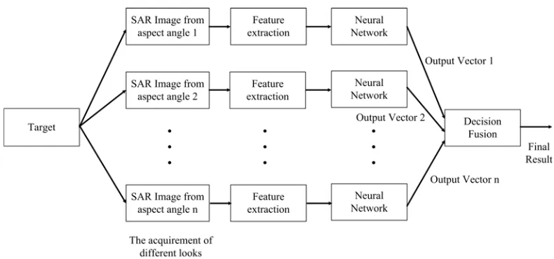
In the multi-look SAR ATR, all looks belong to the same target. A common joint recognition method for NN is to concatenate input features of all looks into a single large-dim vector, acting as the input for the NN training, which has been widely used in the sensor fusion by NN [23]. However, this method will cause the dimension of the vector enormously large after the concatenation, and it is more likely to face the curse of dimensionality. With the increase of the number of looks, the situation will be more serious, which totally decrease the viability of this method. Furthermore, the number of looks may be varied with targets. Thus, different NN structures are required to be trained for the recognition. In a word, an effective joint recognition method for multi-look SAR ATR is in demand.
Figure 3. Neural Network for Multi-look SAR ATR.
Here, the D-S theory of evidence is exerted to combine results and every look’s output vector is treated as BPA. Although, this method only regards every look as individual input and doesn’t exploit the interrelation among these looks, the effect is acceptable especially when the number of looks is small. Furthermore, this method operates quite fast, which perfectly meets the requirement of SAR ATR.
To improve the recognition performance, the result of pose estimation should also be applied in the recognition process. In the process of angle discretization, training data and test data are divided into several classes. For the test data, we try to classify them by training the NN with the training data in the same angle class. Thus, for the NN, aspect angles of the training data and the test data lie in the same angle range, which will remove the interference of aspect angle and make the network focus on the learning of other discriminative features related to the target.
Meanwhile, during the aspect angle discretization, the range of every class is non-lapped and the test sample lying near the class boundary is readily to be classified as other classes. Consequently, the aspect angle range of the training set for the NN may not cover the aspect angle of the test sample. The advantage of the pose estimation will not be exploited since the aspect angle constraint is invalid. To avoid this situation, for the test data belonging to classi, whose aspect angle range is [δi, δi+δ] , the training data in the range of [δi−0.5δ, δi + 1.5δ] are used for the training of NN. In this way, the data near the class boundary are also concerned and the correct aspect angle constraint can be introduced. This idea of how to introduce aspect angle constraint is similar to the method in [24, 25].
3.5. Sparse Representation for Multi-Look SAR ATR with Aspect Angle Constraint
The conclusion from [20] verifies that the introduction of aspect angle constraint can lead to an improvement of recognition rate for SR. For the JSR in [9], all looks are considered as a whole for recognition. This method doesn’t include the information of aspect angle. Here, we try to introduce the constraint of aspect angle for the multi-look SAR ATR.
The process of aspect angle discretization in 3.1 makes all training samples and test samples classified into a certain range of aspect angle. A simple way to achieve the angle constraint is to use train samples which lie in the same angle class as test sample to build the dictionary for SR. However, since the number of train samples of each aspect angle class will drop a lot when the range of aspect angle class decreases. It will be likely to break the foundation of SR that is the dictionary should be over-complete. So, Eq. (6) is adopted first to calculate the sparse coefficients. Then, Eq. (13) is used to get the recognition result.
ˆi= arg min i
Y −Dδia( ˆX)
2 (13)
to not only class i, but also the same angle class as the test data Y, are retained. However, since test sample Y contains many looks, whose aspect angles are different, a comprehensive aspect angle for the whole looks needs to be estimated in order to be applied to multi-look SAR ATR. Because the method in this paper focuses on the pose estimation of single image, and the gap of aspect angle between consecutive looks is considerably small in JSR, the aspect angle of the image in the middle of the test image sequence can be regarded as the angle of the whole looks.
Furthermore, to cover the data lying near the boundary, the same aspect angle range enlarge strategy as 3.4 is utilized for the definition ofδia( ˆX). Thus, the training data of the same angle class, in which the test sample lies, and some data of the adjacent range are both included. After the classification by NN and JSR, decision fusion by summation, which is illustrated in 3.3, is exerted to obtain the final recognition result.
4. EXPERIMENTAL RESULTS
4.1. Experimental Setup and Preprocessing Process
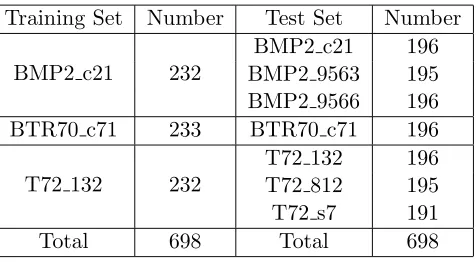
In our experiment, 3 classes (BMP2, BTR70 and T72) of the MSTAR database are used to make up the training set and test set. The MSTAR database consists of X-band images with resolution of 0.3 m ×0.3 m. The training set is captured with depression angle of 17◦, while the depression angle of the test set is 15◦. The training set includes sn c21 for BMP2, sn c71 for BTR70 and sn 132 for T72, and the test set includes all the 7 variants for these three classes. Details about the training and test sets are given in Table 2. Our experiment is run on a 4-core Intel(R) Core(TM) [email protected] GHz CPU with Matlab 2011a.
Table 2. Training set and test set.
Training Set Number Test Set Number
BMP2 c21 232
BMP2 c21 196 BMP2 9563 195 BMP2 9566 196
BTR70 c71 233 BTR70 c71 196
T72 132 232
T72 132 196
T72 812 195
T72 s7 191
Total 698 Total 698
The size of the image in MSATR is 128×128, which is too large to be trained. Firstly, these images are cut into the size of 64×64, which contains only the information of the target. Then, PCA is utilized to reduce the dimension further, in which 99% of variant is kept. After the PCA processing, the original image is transformed into a 540-dim vector, whose size is smaller than the number of training samples. Thus, SR can be applied since the dictionary is over-complete.
4.2. Influence of the Range of Aspect Angle Class
The discretization of aspect angle is a vital process in our paper, which not only provides a rough pose estimation result, but also offers aspect angle constraints for the recognition. The range of aspect angle classes is closely related to the pose estimation accuracy. This experiment evaluates the influence of the range of classes
same NN structure expected for the output layer, which has only 3 units, is utilized. The JSR requires that consecutive looks have little pose differences. Here, the gap is set to 1◦. The number of looks is set to 3 in this experiment. All NNs in our method are optimized by the L-bfgs method.
Table 3. Pose estimation by different method.
The Range of Class PE by NN PE by SR PE by DS PE by DS of Enlarged Range
60◦ 96.70% 94.21% 97.07% 100.00%
45◦ 89.67% 91.94% 92.82% 98.61%
30◦ 85.27% 88.21% 90.04% 97.73%
20◦ 82.05% 85.12% 88.28% 94.65%
10◦ 78.39% 75.82% 80.73% 90.47%
In Table 3, PE is short for “Pose Estimation”. DS is short for “Decision fusion”. “PE by DS of Enlarged Range” means the accuracy of pose estimation when the range of aspect angle class is enlarged by the way in 3.4. It can be seen from Table 3 that the accuracy of pose estimation is reduced with the decrease of the range of aspect angle class. On the one hand, the smaller the range is, the harder it can be classified correctly. On the other hand, the number of data belonging to each class will drop dramatically with the decrease of the range. Thus the size of the training set is relatively small, and the model, especially for NN, cannot be fully trained in this situation. In addition, Table 3 also shows that there are more than 90% of test data, whose aspect angles can be included when the range of corresponding angle class is enlarged. Consequently, it is reliable to treat the pose estimation result as the aspect angle constraint.
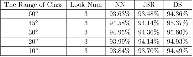
Table 4. Recognition rate with different range of aspect angle class.
The Range of Class Look Num NN JSR DS
60◦ 3 93.63% 93.48% 94.36%
45◦ 3 94.58% 94.14% 95.37%
30◦ 3 94.95% 94.36% 95.60%
20◦ 3 93.99% 94.14% 94.93%
10◦ 3 93.84% 93.70% 94.49%
It can be figured out from Table 4 that our method can reach its best performance when the range of aspect angle class is 30◦. For larger angle range, although the accuracy of pose estimation is high, the constraint of aspect angle is so mild that the classifier will be interfered by samples of other angles, leading the effect of aspect angle constraint to decrease. For smaller angle range, the low accuracy of pose estimation and the lack of training data for each aspect angle class bring down the recognition rate.
4.3. Comparison with Other Pose Estimation Methods
recognition. In the recognition, for the “PE By ED” , the aspect angle range is enlarged to the same extend as ours, that is 15◦ on both sides of the range. For “PE By MI”, the range is enlarged by 10◦ on both sides. For “AAAC”, there is no need to enlarge the range of aspect angle class since the aspect angle of each test sample is precise.
Table 5. Recognition rate with different pose estimation method.
Method Non-PE PE By ED[17] PE By MI[18] Our Method AAAC
PE Accuracy — 90.22% 94.80% 90.04% 100.00%
NN 93.40% 94.80% 95.09% 94.95% 95.31%
JSR 93.18% 94.65% 94.73% 94.51% 94.87%
DS 94.00% 95.60% 95.76% 95.60% 96.04%
PE Time (s) — 16.38 41.91 9.34 —
In Table 5, we can find that all methods with constraints of aspect angle are superior to the method without, pointing out that the inclusion of the information of aspect angle can obviously boost the recognition performance. Besides, the accuracy of pose estimation by our method is inferior to other methods. However, the gap of the final recognition rate between our method and other methods is considerably narrower, which can be ignored, than the gap of the pose estimation accuracy. Thus, it can be concluded that the prediction of aspect angle by our pose estimation method is reliable enough to meet the requirement of the recognition process. In addition, the pose estimation via our method is about 2 times faster than the way of ED and 4.5 times faster than the way of MI. Although in this experiment, no matter which method is adopted, the time of pose estimation is less than 1 minute, the training set and test set in practical situation will be dramatically larger than in our experiment, indicating that large amounts of time will be consumed, and consequently, our method will be strikingly significant with more time saved.
4.4. Comparison with Other Multi-Look SAR ATR Methods
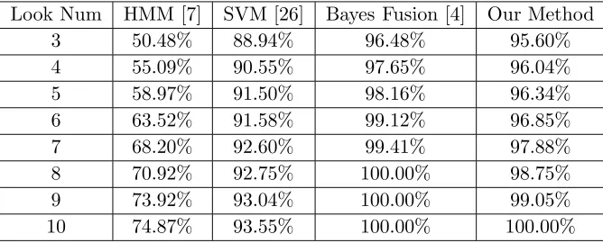
In this experiment, with the increase of number of looks, two multi-look SAR ATR methods, i.e., HMM [7] and SVM [26], are evaluated based on the same feature as our paper. In our method, the range of aspect angle class in discretization is fixed to 30◦. Moreover, another decision fusion method, which is based on Bayes rule [4], is adopted to fuse the recognition result by NN and JSR in our method. From Table 6, it can be figured out that our method outperforms HMM and SVM, and the recognition rate is obtained as 100% via our method when the number of looks is 10. Meanwhile, the result of Bayesian fusion is superior to our method, but it demands the correct class of every test sample, which definitely decreases its practical value.
Table 6. Recognition rate with different number of looks.
Look Num HMM [7] SVM [26] Bayes Fusion [4] Our Method
3 50.48% 88.94% 96.48% 95.60%
4 55.09% 90.55% 97.65% 96.04%
5 58.97% 91.50% 98.16% 96.34%
6 63.52% 91.58% 99.12% 96.85%
7 68.20% 92.60% 99.41% 97.88%
8 70.92% 92.75% 100.00% 98.75%
9 73.92% 93.04% 100.00% 99.05%
5. CONCLUSION
In SAR ATR, it is a common way to boost recognition rate by introducing the information of pose. Existing methods for pose estimation lack the contribution of decision fusion. Besides, for SAR ATR, there is a demand for the combination of the feature fusion and the decision fusion. As for these problems, a two-level decision fusion of NN and SR for multi-look SAR ATR is proposed in this paper to combine these advantages. Firstly, NN and SR are exploited to evaluate aspect angles of the test data. Then, first-level decision fusion is acted to combine these results. Based on the introduction of aspect angle constraint, multi-look SAR ATR is completed by these two classifiers respectively. After that, second-level decision fusion is exerted to obtain the final result. Experimental results show that our method can outperform some other pose estimation methods and multi-look SAR ATR methods.
For the method of multi-look SAR ATR by NN in our paper, the recognition of every look is individual, and the fusion is applied after all looks finishing their recognition processes. This method does not depend on the interrelation among different looks. In the future, we will explore a new method for multi-look SAR ATR based on NN via the interrelation
REFERENCES
1. O’Sullivan, J. A., et al., “SAR ATR performance using a conditionally Gaussian model,” IEEE Transactions on Aerospace and Electronic Systems, Vol. 37, No. 1, 91–108, 2001.
2. Brown, M. Z., “Analysis of multiple-view Bayesian classification for SAR ATR,” AeroSense 2003. International Society for Optics and Photonics, 265–274, 2003.
3. Ruta, D. and B. Gabrys, “An overview of classifier fusion methods,” Computing and Information Systems, Vol. 7, No. 1, 1–10, 2000.
4. Liu, H. and S. Li, “Decision fusion of sparse representation and support vector machine for SAR image target recognition,” Neurocomputing, Vol. 113, 97–104, 2013.
5. Yu, X., Y. Li, and L. C. Jiao, “SAR automatic target recognition based on classifiers fusion,”2011 International Workshop on Multi-Platform/Multi-Sensor Remote Sensing and Mapping (M2RSM), IEEE, 1–5, 2011.
6. Ranney, K. I., H. Khatri, and L. H. Nguyen, “SAR prescreener enhancement through multi-look processing,” Defense and Security. International Society for Optics and Photonics, 1065–1072, 2004.
7. Albrecht, T. W. and S. C. Gustafson, “Hidden Markov models for classifying SAR target images,”
Defense and Security. International Society for Optics and Photonics, 302–308, 2004.
8. Albrecht, T. W. and K. W. Bauer, Jr., “Classification of sequenced SAR target images via hidden Markov models with decision fusion,” Defense and Security. International Society for Optics and Photonics, 306–313, 2005.
9. Zhang, H., et al., “Joint sparse representation based automatic target recognition in SAR images,”
SPIE Defense, Security, and Sensing. International Society for Optics and Photonics, 805112– 805112, 2011.
10. Morgan, D. R. and T. D. Ross, “A Bayesian framework for ATR decision-level fusion experiments,”
Defense and Security Symposium. International Society for Optics and Photonics, 65710C–65710C, 2007.
11. Ettinger, G. J. and W. C. Snyder, “Model-based fusion of multi-look SAR for ATR,” AeroSense 2002. International Society for Optics and Photonics, 277–289, 2002.
12. Huan, R. and Y. Pan, “Decision fusion strategies for SAR image target recognition,” IET radar, Sonar &Navigation, Vol. 5, No. 7, 747–755, 2011.
13. Huan, R.-H. and Y. Pan, “Target recognition for multi-aspect SAR images with fusion strategies,”
Progress In Electromagnetics Research, Vol. 134, 267–288, 2013.
15. Kaplan, L. M. and R. Murenzi, “Pose estimation of SAR imagery using the two dimensional continuous wavelet transform,”Pattern Recognition Letters, Vol. 24, No. 14, 2269–2280, 2003. 16. Voicu, L. I., R. Patton, and H. R. Myler, “Multicriterion vehicle pose estimation for SAR ATR,”
AeroSense’99. International Society for Optics and Photonics, 497–506, 1999.
17. Sun, Y., et al., “Adaptive boosting for SAR automatic target recognition,” IEEE Transactions on Aerospace and Electronic Systems, Vol. 43, No. 1, 112–125, 2007.
18. Principe, J. C., D. Xu, and J. W. Fisher, III, “Pose estimation in SAR using an information theoretic criterion,”Aerospace/Defense Sensing and Controls. International Society for Optics and Photonics, 218–229, 1998.
19. Roberts, D. J., “Applications of artificial neural networks to synthetic aperture radar for feature extraction in noisy environments,” Diss. California Polytechnic State University San Luis Obispo, California, 2013.
20. Xing, X., et al., “SAR vehicle classification based on sparse representation with aspect angle constraint,” Eighth International Symposium on Multispectral Image Processing and Pattern Recognition. International Society for Optics and Photonics, 89180K–89180K, 2013.
21. Ng, A., “Sparse autoencoder,” CS294A Lecture notes, Vol. 72, 2011.
22. Rennie, J. D. M., “Pose estimation in SAR using an information theoretic criterion,” Diss. Massachusetts Institute of Technology, 2001.
23. Azouzi, R. and M. Guillot, “On-line prediction of surface finish and dimensional deviation in turning using neural network based sensor fusion,” International Journal of Machine Tools and Manufacture, Vol. 37, No. 9, 1201–1217, 1997.
24. Principe, J., Q. Zhao, and D. Xu, “A novel ATR classifier exploiting pose information,”Proceedings of Image Understanding Workshop, 833–836, 1998.
25. Zhao, Q. and J. C. Principe, “Support vector machines for SAR automatic target recognition,”
IEEE Transactions on Aerospace and Electronic Systems, Vol. 37, No. 2 643–654, 2001.