Analysis of Step-Loaded Open Rectangular Grating Slow-Wave
Structures for MM-Wave Traveling-Wave Tubes
Chengfang Fu1, *, Yanyu Wei2, Bo Zhao1, Yudong Yang1, and Yongfeng Ju1
Abstract—The open rectangular grating with step-loaded slow-wave structure (SWS), a type of all-metal SWS for high power wide band mm-wave wave traveling wave tubes (TWT) is presented in this paper. By using the jumping conditions at the interface of two neighboring steps and single-mode approximation (SMA) field matching theory, the dispersion equation and coupling impedance of this SWS were obtained. Then the obtained complex dispersion equation was numerically calculated, and the slow-wave characteristics of the fundamental wave of this structure were discussed. Moreover, the calculation results by our theory were accordant with the simulation data obtained by the 3D electromagnetic simulation software HFSS. The numerical calculation results show that the dispersion characteristics and coupling impedance are notably improved by loading the steps. And the working bandwidth may be the widest when the thickness of the step is about equal to the thickness of the groove depth. The proper design parameters can be optimized to meet the needs of high frequency characteristics with wide bandwidth and high output power. The present study will be useful for further research and design of this kind of high frequency system.
1. INTRODUCTION
With the rapid development of electronic counter, radar, space research, etc., the millimeter (mm) and sub-mm wave frequencies have come to be a hot research band for channel capacity. Traveling wave tubes (TWT), which is a kind of important microwave source both in military and civil areas for possessing advantages of wide bandwidth and high power, cannot be replaced in the mm wave band [1, 2]. Slow-wave structure (SWS) is a key part in TWT because it directly determines the TWT’s properties. But the physical dimension of SWS for mm wave devices becomes too small to manufacture easily, which makes it a current research topic to find a new type of SWS for mm wave TWT. The rectangular grating is an ideal candidate SWS for mm wave TWT for the advantages of the scalability to smaller dimension, interaction with sheet beam, which may reach the peak powers as high as several hundreds of kilowatts in high frequency band (100 to 300 GHz). The open rectangular grating is a deformation of rectangular grating by disposing the metal short circuit side plates, which is open in the transverse direction. This kind of SWS has attracted much interest due to its all-metal structure features: super thermal capacity, low loss, high precision of manufacturing and assembling, high power capacity, compact dimension, which make it to be applied as interaction circuits for mm wave frequency especially. It is proved in [3–6] that the larger the groove depth is, the slower the phase velocity of the electromagnetic wave is. In other words, the groove depth should be increased to obtain slow electromagnetic wave which should be synchronous with the electron beam inside TWT, but this may cause remarkable skin dissipation, which will decrease the output power of the open rectangular grating TWT. To improve the high frequency characteristics of open rectangular grating SWS in the case of
Received 8 October 2015, Accepted 27 November 2015, Scheduled 14 December 2015 * Corresponding author: Chengfang Fu (fchff[email protected]).
1 Faculty of Electronic Information Engineering, Huaiyin Institute of Technology, Huai’an 223003, China. 2 School of Physical
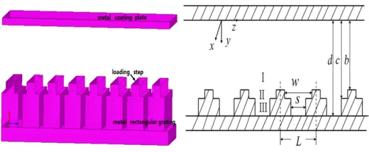
Figure 1. 3D Model and dimensional parameters of an open step-loaded rectangular grating SWS.
certain groove depth, considering of the advantages of loading steps, an open step-loaded rectangular grating structure is presented, illustrated in Fig. 1 [7, 8].
This paper is arranged as follows. Section 1 present a brief introduction. In Section 2, the field expressions, dispersion equation and coupling impedance expression are derived. In Section 3, the theoretical results are compared with those by HFSS (Ansoft Corporation). The numerical calculation and discussions are shown in Section 4. Finally, a short conclusion is given.
2. ANALYSIS
2.1. Dispersion Characteristics of the Open Step-Loaded Rectangular Grating
The open step-loaded rectangular grating SWS is shown in Fig. 1. In Fig. 1, the structure should be divided into three regions: interaction regionI (0≤y≤b), gap region II (b≤y≤c) and groove region III (c≤y≤d). b,c and dare the distances of the top surface of the step, bottom surface of the step, and groove bottom to the top metal plate, respectively. L, s and w are the structure period, groove width and step gap, respectively, andais the width of the rectangular waveguide. The electromagnetic wave propagates along the step-loaded groove and is slowed down inz-direction. When the velocity of the wave is synchronous with the sheet beam, the electromagnetic energy is transferred from the beam to the slow wave, and the wave is amplified.
2.1.1. Field Distributions
For the structure shown in Fig. 1, the widthais much larger than the heightb, and they are both much smaller than the wavelength in the vacuumλ0. The structure should be treated to be infinitely wide,
and the end-effect should be omitted [4]. The slow-wave mode supported by this structure is TM (that is, mode E) which does not vary with x. Both slow and fast waves are excited due to the closeness of the structure. Each of these waves consists of an infinite sum of space harmonics on account of the periodicity of the structure. Omitting the time dependence exp(jωt), whereω is the angular frequency, according to Floquent’s theorem, the fields in region I can be written as followings under Cartesian coordinates (x,y,z):
⎧ ⎪ ⎪ ⎪ ⎪ ⎪ ⎪ ⎪ ⎪ ⎪ ⎨ ⎪ ⎪ ⎪ ⎪ ⎪ ⎪ ⎪ ⎪ ⎪ ⎩
HxI(y, z) = ∞
n=−∞
AInFnI(y) +BInGIn(y)e−jβnz
EIz(y, z) = jωμ0 k02
∞
n=−∞
AInFnI(y) +BnIGnI(y)
e−jβnz
EIy(y, z) =−ωμ0 k02
∞
n=−∞
βnAInFnI(y) +BnIGIn(y)e−jβnz
(1)
where AIn and BnI are the amplitude factors of the nth space harmonic, where k0 is the propagation
permittivity of free space and μ0 the permeability of free space. If ξ2n = βn2 −k02 > 0, the field
represents the slow-wave mode, while FnI(y) = sinh(ξny), GIn(y) = cosh(ξny), FnI(y) = ξncosh(ξny), GnI(y) = ξnsinh(ξny); If ζn2 = βn2 − k02 < 0, the field represents the fast wave mode, while
FnI(y) = sin(ζny),GnI(y) = cos(ζny), FnI(y) =ζncos(ζny),GnI(y) =−ζnsin(ζny).
In gap and groove regions (II and III), we assume that the electric field has a component in the z-direction only and is homogenous across the breadth of the gap and groove. According to the single-mode approximation (SMA) [4, 5], it is reasonable to treat the waves as standing waves on conditions that the groove width and step gap are much smaller than the wavelength in vacuum, so the axial propagation constants are zero, i.e., γi =k0 (i=II orIII). Then, the field expressions may be written
as follows: ⎧
⎪ ⎪ ⎨ ⎪ ⎪ ⎩
Hxi =Ai0sin(k0y) +B0icos(k0y)
Ezi = jωμ0 k0
Ai0cos(k0y)−B0isin(k0y)
Eyi =Hyi=Exi=0
(2)
whereAi0 and B0i (i= II orIII) are the amplitude factors of the field expressions.
2.1.2. Dispersion Equation
The boundary conditions at the metal surface require that the tangential component of the electric field must vanish, i.e.,
(1)
At y= 0 : EzI = 0; (3)
(2)
At y=d: EzIII = 0; (4)
(3) The matching conditions aty=bare that the tangential electric and magnetic fields are continuous across the gapy=b, 0< z < w, and the tangential electric field vanishes on the upper faces of the teeth, i.e., at y=b forw < z < L, orNL+w < z <(N + 1)L in general. Thus the conditions at the interface of regionI and region II can be described as [4]:
EzI|y=b =
EzII|y=b
0
N L < z < N L+w
N L+w < z < N L+L (5) HxI|y=b =HxII|y=b N L < z < N L+w (6)
(4) The electromagnetic fields matching method cannot directly be applied aty=c, because only the Ez component of the electrical field is considered in region II and III. Furthermore, the width of these two regions varies fromwto s, which will cause the high order decay modes, and these modes mainly exist at the interface. So the matching conditions should be substituted for the ones that voltage and current is continuous [9]
VzII = VzIII (7) JyII = JyIII −B1·VzIII (8)
where [10],
B1 = jωC1 (9)
C1 = ε 0
2π
α2+ 1 α ln
1 +α 1−α −2 ln
4α 1−α2
(10)
α = w/s (11)
To utilize the above matching condition, s < 0.2λ0 should be satisfied. C1 is the discontinuity
unit length can be described as in Eqs. (12) and (13)
VzII =EzII·w
VzIII =EzIII ·s (12)
JyII =HxII
JyIII =HxIII (13) So, the matching conditions at the interface of regionII and III can be described as:
EzII|y=c w=EzIII|y=cs (14)
HxII|y=c =HxIII|y=c −jωC1EzIII|y=c (15)
Substituting the field expressions of each region into the above boundary conditions (3)–(15) to eliminate the amplitude constants, we obtain the dispersion equation of the open step-loaded rectangular grating slow-wave structure: ∓w L ⎧ ⎪ ⎪ ⎪ ⎨ ⎪ ⎪ ⎪ ⎩
n=∞
n=−∞
k0 ξn ⎛ ⎜ ⎜ ⎝ sin βnw 2
βnw 2 ⎞ ⎟ ⎟ ⎠ 2
GIn(ξnb) GnI(ξnb)
⎫ ⎪ ⎪ ⎪ ⎬ ⎪ ⎪ ⎪ ⎭
AII0 cos(k0b)−B0IIsin(k0b)
=AII0 sin(k0b) +BII0 cos(k0b) (16)
where
AII0 = B0III
s w
GII0 (γ2c)
F0III(γ3d)
P0(c, d)− G
II
0 (γ2c)
F0III(γ3d)
Q0(c, d)−wsC1Z0 G
II
0 (γ2c)
F0III(γ3d)
P0(c, d)
B0II = B0III
−s
w
F0II(γ2c)
F0III(γ3d)
P0(c, d)− F
II
0 (γ2c)
F0III(γ3d)
Q0(c, d) +wsC1Z0 F
II
0 (γ2c)
F0III(γ3d)
P0(c, d)
P0(c, d) = G
III
0 (γ3c)F
III
0 (γ3d)−F
III
0 (γ3c)G
III
0 (γ3d)
Q0(c, d) = GIII0 (γ3c)F
III
0 (γ3d)−F0III(γ3c)G
III
0 (γ3d)
where upper and lower signs “±” in Eq. (16) represent the slow-wave and fast-wave modes, respectively. If w/s = 1, i.e., there is no step loaded in this structure, Eq. (16) can be reduced to the dispersion equation of the open rectangular grating structure [11].
2.2. Coupling Impedance
From Pierce’s theory [12],Kc(n) is the coupling impedance for thenth space harmonic wave and defined as
Kc(n) =Ezn·Ezn∗ /
2 (βn)2P
(17) where, Ezn is the longitudinal component of the electric field of the nth space harmonic wave at the position of the electron beam, andE∗zn is its conjugate component. We can obtain
Ezn·Ezn∗ = ω
2μ2 0
k40
γn2(BnI)2(GmI(γnye))2 (18)
Define P as the total flow along thez-axis through the whole circuit system P =
n
PnI+PII+PIII (19)
region I and can be written as
P = n
PnI = aωμ0 2k20
∞
n=−∞
βn(BnI)2Int(I) (20)
where, Int(I) =
⎧ ⎪ ⎪ ⎨ ⎪ ⎪ ⎩
2 b +
sinh(2ξnIb) 4ξnI
ξnI2 >0 2
b +
sin(2ζnIb) 4ζnI
ζnI2<0
(21)
Using the results of the dispersion relations and putting expressions (18) and (21) to (17), we may get the coupling impedance. Here the coupling impedance is calculated by assuming that a sheet beam passes through the surfaces of the steps, i.e., the position of the electron beam is aty=b.
3. 3D SIMULATION
In order to check the theory above, the three-dimensional electromagnetic simulation software HFSS is used to simulate a certain structure for comparison. Fig. 2 shows the dispersion characteristics and coupling impedance of the fundamental space harmonic wave of a step-loaded open rectangular grating SWS. The smooth curve represents the theoretical results; the square points denote the results obtained from HFSS in Fig. 2. It is obvious that the HFSS simulation data are in good agreement with the theoretical calculations in higher frequency, which verifies that our theoretical method is effective. On the other hand, in lower frequency band there is a certain discrepancy between the theory and simulation data, which is caused by the treatment of the infinite width of the rectangular cross-section in the theoretical analysis, while in the software simulation the width is finite. And research shows that the results converge when the SWS’s width is 8 times of the grating period [11]. Here the width in our simulation is applied as 8 times of period. In the whole frequency band, the results calculated by the theory method and simulation differ from each other by a maximum of 5%, which justifies that our theoretical method is correct.
(a) (b)
Figure 2. (a) Dispersion characteristics. (b) Coupling impedance of an open step-loaded rectangular grating SWS with dimensions (unit: mm): d= 7.2,c= 4.8, b= 4, L= 2, w= 1.2, s= 0.4,a= 16.
4. NUMERICAL CALCULATIONS AND DISCUSSION
The dispersion Eq. (16) is a complex transcendental equation including the sum of infinite series, which can be solved by numerical calculation. It can be proved that the series converges rapidly as the term number n increases. A sufficiently accurate solution with the relative error less than 10−6 can be
seven terms (n <=3 ) are kept in the summations of Eq. (16). In the following discussion, we consider the β0L/πas independent variable, andk0a,vp/c,Kc(n)are dependent variables. Fig. 3–6 are the numerical
calculation results using above method to resolve the dispersion relations and coupling impedance of the fundamental space harmonic wave.
Figures 3(a)–(b) show the effects of gap widthwon the dispersion curves and coupling impedance. It is obvious that the dispersion curves become flatter, and the operating band moves to the higher frequency range as the gap width w increases, but the coupling impedance decreases clearly. In other words, the bandwidth increases with increasingw. When gap width w is equal to the groove width, as curve A shown in Figs. 3(a)–(b), the structure represents a step-unloaded one, and the dispersion curve is the steepest and the working band the narrowest, but the coupling impedance is the largest. Generally speaking, loading steps can weaken the dispersion and increase the bandwidth, but the corresponding coupling impedance is decreased.
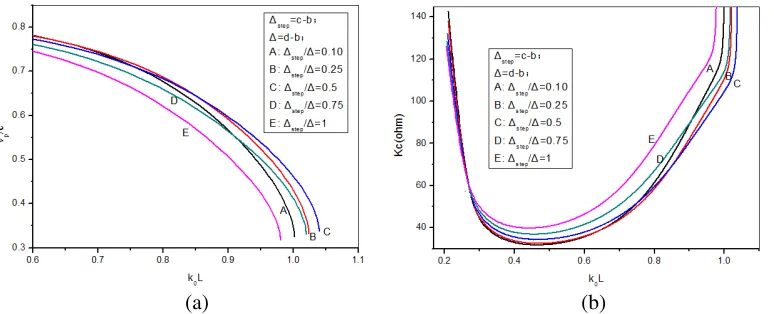
Figures 4(a)–(b) show the influence of the thickness (c−b)/(d−b) of the loading steps on the slow-wave characteristics. It can be drawn from Fig. 4(a) that the phase velocity becomes larger, and the bandwidth increases as the thickness of the loading steps increases under certain (d−b), when a certain thickness of the loading steps is reached, the phase velocity changes oppositely. In Fig. 4(b) it is obvious
(a) (b)
Figure 3. (a) Effect of gap width w on the normalized phase velocity of the fundamental wave. (b) Effect of gap width w on the coupling impedance. Calculation parameters: d/L = 3.6, c/L = 2.4, b/L= 2,s/L= 0.2.
(a) (b)
(a) (b)
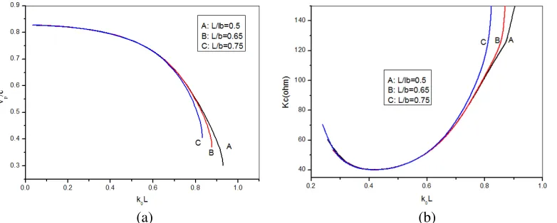
Figure 5. (a) Effect of grating periodLon the normalized phase velocity of the fundamental wave. (b) Effect of grating period L on the coupling impedance. Calculation parameters: d/b = 1.8, c/b = 1.2, s/b= 0.25, w/b= 0.3.
(a) (b)
Figure 6. (a) Effect of grating depth on the normalized phase velocity of the fundamental wave. (b) Effect of grating depth on the coupling impedance. Calculation parameters: b/L= 2.0, c= (b+d)/2, s/L= 0.6, w/L= 0.5.
that the coupling impedance decreases firstly then increases. In Figs. 4(a)–(b), curve E is the dispersion and coupling impedance of the open rectangular grating unloaded step, which is the (c−b)/(d−b) = 1. Compared with the unloaded step open rectangular grating, loading step to the open rectangular grating can broaden the working bandwidth notably, and the coupling impedance is decreased correspondingly. Furthermore, there is an optimal thickness of the loading step ((c−b)/(d−b))∼0.5 to achieve the high frequency characteristics with the widest bandwidth.
Figures 5(a)–(b) show the phase velocity and coupling impedance with frequency on variant grating periodL, respectively. To simplify the analysis, the loaded steps thickness (c−b) is kept equal to the groove thickness (d−c). It is clear that the grating periodLhas no obvious influence on the dispersion and coupling impedance except for the central frequency moving towards the lower frequencies with increasing grating periodL, and the corresponding coupling impedance increases a little.
5. CONCLUSIONS
In this paper, the step-loaded open rectangular grating SWS has been presented for mm-wave TWT. The slow-wave characteristics including dispersion relation and the expression of the coupling impedance are derived applying SMA. Then the dispersion equation and coupling impedance are numerically calculated with varied physical dimensions, and the numerical results are in good agreement with the data obtained from HFSS, which supports the theory. It can be concluded from the theoretical analysis that loading-step will flatten the dispersion to a certain degree and broaden the working bandwidth compared with the structure unloading steps. And the step thickness (c−b) is about equal to the groove depth (d−c) to achieve the high frequency characteristics with the widest working bandwidth. The study will provide a theoretical basis for further research and design of this kind of slow-wave structure for mm-wave TWT.
ACKNOWLEDGMENT
This work was supported by the National Natural Science Foundation of China (Grant No. 61401173).
REFERENCES
1. Fu, C., H. Zhu, and Y. Wei, “The small signal analysis of a thicker helix traveling-wave tube under the helical coordinate system,” High Power Laser and Partical Beams, Vol. 26, No. 3, 033002(6), 2014.
2. Kory, C., L. Ives, J. Booske, et al., “Novel TWT interaction circuits for high frequency application,” International Vacuum Electron Conference 2004, 51–52, 2004.
3. Louis, L. J., J. E. Scharer, and J. H. Booske, “Collective single pass gain in a tunable rectangular grating amplifier,”Physics of Plasmas, Vol. 5, No. 5, 2797–2805, 1998.
4. Collin, R. E., Foundations for Microwave Engineering, 2nd Edition, 571-580, Wiley-IEEE Press, New York, 2001.
5. Maragos, A. A., Z. C. Ioannidis, and I. G. Tigelis, “Dispersion characteristics of a rectangular waveguide grating,”IEEE Trans. on Plasma Science, Vol. 31, No. 3, 1075–1082, 2003.
6. Gong, Y.-B., Z.-G. Lu, G.-J. Wang, et al., “Study on mm-wave rectangular grating traveling wave tube with sheet-beam,” J. Infrared Millim. Waves, Vol. 25, No. 3, 173–178, 2006.
7. Lu, Z.-G., Y.-Y. Wei, Y.-B. Gong, et al., “Study on step-loaded rectangular waveguide grating slow-wave system,” J. Infrared Millim. Waves, Vol. 25, No. 3, 349–354, 2006.
8. Yue, L., W. Wnag, Yu. Gong, et al., “Analysis of coaxial ridged disk-loaded slow-wave structures for relativistic traveling wave tubes,”IEEE Trans. on Plasma Science, Vol. 32, No. 3, 1086–1092, 2004.
9. Wang, W. X., G. F. Yu, and Y. Y.Wei, “Study of the ridge-loaded helical groove slow-wave structure,” IEEE Trans. Microwave Theory Tech., Vol. 45, No. 8, 1689–1695, 1997.
10. Ramo, S., J. Whinnery, and T. V. Duzer, Fields and Waves in Communication Electronics, 573– 579, Wiley, New York, 1965.
11. Liao, M.-L., Y.-Y. Wei, Y. Huang, et al., “Study on mm band open rectangular waveguide grating,”The 17th Annual Seminar Conference on Military Microwave Tube, 272–276, The Chinese Electronic Society, Yichang, 2009.