Robust Adaptive Sidelobe Canceller Using SV Mismatch Estimation

Robust Adaptive Sidelobe Canceller Using SV Mismatch Estimation

Zhen Tao1, 2, *, Mingwei Shen1, 2, Chao Liang2, Di Wu3, and Daiyin Zhu3

Abstract—In this paper, to overcome signal-to-interference-and-noise ratio (SINR) performance degradation in the presence of steering vector (SV) mismatch between beam pointing and desired signal’s SVs, we study the mismatch of SV with adaptive uncertainty level. This estimation is derived based on the geometrical interpretation of the mismatch and can be expressed as a simple closed-form expression as a function of the presumed SV and the signal-subspace projection. Then, the adaptive uncertainty algorithm self-adjusts the uncertainty sphere according to the estimated mismatch SV at each iteration. Finally, the robust adaptive sidelobe canceller (R-IASLC) algorithm can accurately evaluate the mismatches between the actual and presumed SVs and improve the target SINR. Simulation results verify the effectiveness of this method.

1. INTRODUCTION

Adaptive digital beamforming (ADBF) [1, 2] is an important technique for narrowband noise jamming suppression in digital array applications. Jamming signals are the result of intentional introduction of a noise-like waveform into the receiver. For most ADBF algorithms, the adaptive weight is calculated for maximizing the output signal-to-noise-ratio (SNR), which is able to null out the jamming sufficiently, but meanwhile may result in a disadvantage of high sidelobe level of the adaptive beam pattern. In [3], an improved adaptive sidelobe canceller (IASLC) method can not only suppress the sidelobe level, but also reduce the processor’s degrees of freedom, which consequently results in a fast convergence rate and a much lower computation load. However, traditional ADBF techniques are sensitive to mismatches between the presumed and actual SVs and may result in substantial degradation in their performance [4, 5], and IASLC method is no exception. Additionally, the mismatch of SV will induce gain loss of the desired signal which brings about the dramatic degradation of the output SINR.

In these years, improving the robustness of the beamformer against the mismatch of SV is becoming an essential requirement, and several contributions have been proposed to work on it [6, 7]. Against the direction of arrival (DOA) [8, 9] mismatch, the most common technique is to delimit one set of unity-gain constraints for a small range of angles around the presumed look direction. Nevertheless, this technique critically degrades the anti-interference performance. Therefore, to improve the IASLC performance in the presence of SV mismatch between beam pointing and desired signal’s SVs, we study the mismatch of SV with adaptive uncertainty level. At each iteration, the uncertainty level is readjusted, and the estimation SV is updated according to the new uncertainty level. The iteration converges when the uncertainty level approximates zero. The estimation is based on the idea that the mismatch vector can be decomposed into components that lie in the signal-plus-interference subspace and the noise subspace. The signal component is conveniently calculated as a function of the signal-subspace projection of the presumed SV, while the noise component is calculated from its orthogonal projection. Ultimately, the optimum weights of arrays can be worked out thereafter.

Received 8 January 2018, Accepted 2 February 2018, Scheduled 12 March 2018

* Corresponding author: Zhen Tao ([email protected]).

1 _{College of Computer and Information Engineering, Hohai University, Nanjing 211100, China.} 2 _{Science and Technology on}

This paper is organized as follows. In Section 2, we formulate the principle of IASLC. In Section 3, we study the improved R-IASLC algorithm. The validity of the method is confirmed by the simulation results in Section 4. Finally a brief conclusion is drawn in Section 5.

2. PRINCIPLE OF IASLC

Let us consider a uniform linear array (ULA) [10] with M sensors impinged by K + 1 narrowband uncorrelated signals (one desired signal and K interferences). The signal received can be written as

X=S+i+n. Where S=a(θ0)s0,i=

K

k=1

a(θ_k)s_k, andn denote M×1 vectors of the desired signal,

interference, and noise, respectively. Moreover,a(θ0) and {a(θk)}Kk=1 are, respectively, steering vectors

of the desired signal and interferences. a(θ) = [ 1, ej2πλ−1dsinθ, . . . , ej2πλ−1(M−1)dsinθ ]T withλ,d, andθdenoting the carrier wavelength, inter-sensor spacing, and direction-of-arrival (DOA) respectively, [·]T donating the matrix transpose.

The auxiliary measurements are weighted and combined to form the high gain sum beam output, Z=a(θ0)HX. Assuming that there areK noncoherent jamming sources, the outputs of auxiliary beams

can be expressed as

C=FH_KX (1)

where FK = [ SK1 SK 2 · · · SK K ] comprises the auxiliary beamforming weights, and SK i = [ 1 ej2πdλ sinθK i · · · ej2πdλ (M−1) sinθK i ]T is theith auxiliary beam steering vector with respect to the direction of the ith jamming source. The outputs of auxiliary beams can be employed to cancel the sidelobe interference received in the quiescent sum beam. The adaptive weight can be solved as

WRD =R−_C1RCZ (2)

whereRC =E[CHC],RCZ =E[ZHC], which are usually obtained by the sample average in the actual radar or communication system.

We can see that when there is a mismatch between beam pointing and actual SVs [11, 12], the output SNR of the target will have a huge loss in Fig. 1. To improve the output SNR of IASLC, we need to further modify the SV of IASLC to correct weight vector. An improved IASLC algorithm will be shown in the following parts.

6 6.2 6.4 6.6 6.8 7 7.2 7.4 7.6 7.8 8 0

10 20 30 40 50 60 70 80

beam pointing (°)

output SNR (dB)

Figure 1. Mismatch output versus beam

pointing.

3. STEERING VECTOR MISMATCH ESTIMATION FOR R-IASLC ALGORITHM

The adaptive beamforming problem [6, 13, 14] is essentially to design the optimal weight vector wthat minimizes the interference-plus-noise output power while maintaining unity response of the desired signal.

min

w w

H_{Rw subject to w}H_{a(t) = 1 (3)}

where a(t) = [ 1 ej2πdλ sint · · · ej2πdλ (M−1) sint ]T, a(t) is the desired signal steering vector, t the desired signal DOA, and R the interference-plus-noise covariance matrix.

When there is a match between the actual and presumed SVs (denoted as ¯a(t)), the signal subspace is the subspace that is spanned by the q principal eigenvectors of R, and the projection matrix to the subspace can be expressed as U_rUH

r , where q denotes the total number of signal-plus-interference impinging on the array. However, when there is a mismatch between the actual and presumed SVs [15– 18] as shown in Fig. 2, the proposed estimate of the signal subspace is given by

Ur(Δ) = [P{Q(Δ)}[ u1 . . . uq ]] (4) where the additional eigenvector is calculated from the principal eigenvector of Q(Δ) : P{Q(Δ)}. Let Q(Δ) denote the positive definite matrix

Q(Δ) =

Δ 2

−Δ 2

¯

a(ϕ+φ)¯aH(ϕ+φ)dφ (5)

where ϕ denotes the look-direction; Δ defines the spatial sector assumed to represent the range of the angular location of the desired signal; u_m(1 ≤ m ≤ q) is the mth eigenvectors of R with the corresponding eigenvalues sorted in decreasing order. When the SNR is sufficiently high, Δ = 0 and U_r(Δ) reverts to U_r. Therefore, the beamformer’s weight can be designed given the norm of the mismatch vector by solving

min

a a(t)

H_R−1_{a(t) subject to a(t)−¯a(t)}

2 ≤ε (6)

where ε specifies the uncertainty level, and ₂ defines the l2 norm. In order to avoid convergence

of formulation in Eq. (6) to zero, we must comply with ε ≤ a¯(t)2₂. The solution to Eq. (6) can be obtained using the Lagrangian multiplier method,

L(a(t), μ) =aH(t)R−1a(t) +μ

a(t)−¯a(t)2₂−ε

subject to ∂L(a(t), μ)

∂a(t) = 0 (7)

Then we get the optimal desired signal SV,

ˆ a(t) =

R−1 μ +I

−1

¯

a(t) = ¯a(t)−(I+μR)−1a¯(t) (8)

where the Lagrange multiplier μis obtained by solving: g(μ)≡ (I+μR)−1¯a(t)2₂=ε.

Let ˆedenote the mismatch vector between the presumed and actual SVs, defined as ˆe=a(t)−a¯(t). It is shown that ˆecan be estimated as the decomposition into nonzero pairwise orthogonal vectors that lie in the signal and noise subspace, denoted as ˆe_Ur and ˆe_⊥Ur, respectively. Thus, we can deduce a closed-form expression of the mismatch estimate ˆe,

ˆ

e= ˆe_Ur + ˆe_⊥Ur =

_√

M

U_rUH

r a¯(t)2

−2 U_rUH_r a¯(t) + ¯a(t) (9)

If Δ is set correctly,U_r(Δ) will include both the desired signal and interferences components, and the length of the mismatch vector is minimum. Thus, Δ can be found from minimizing the length of ˆe

Δ = arg minˆe(U_r(Δ))₂ Δ≥0 (10)

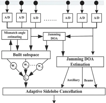
The main idea of the proposed R-IALSC method is to build the mismatch vector, which can be decomposed into components that lie in the signal-plus-interference subspace and noise subspace. Then, R-IASLC algorithm uses auxiliary beams instead of auxiliary elements for adaptive sidelobe jamming cancelation, and some a prior knowledge about jamming sources, such as the interference number and locations, is also required to adaptively construct the auxiliary beams. The principle of robust ADBF algorithm is illustrated in Fig. 3.

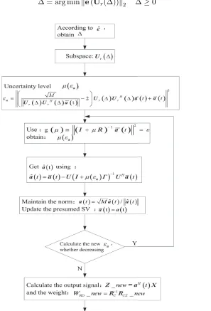
The flowchart of R-IASLC is shown in Fig. 4 for matching between the actual and presumed SV, whereμ(ε_a) denotes the Lagrange multiplier, and diag{Γ}are the eigenvalues of R. The columns ofU contain eigenvectors ofR, and Znew is a new sum beam output and W_RD new a weight of R-IASLC.

4. SIMULATION RESULTS AND ANALYSIS

In this section, we show numerical examples based on the simulated airborne radar clutter data, and the radar system parameters are listed in Table 1.

Table 1. Parameters of radar simulation.

Number of elements 64

Elements spacing 1/2

Bandwidth 5 MHz

Interference to noise ratio 20 dB DOA of the desired signal 7◦

Range of main beam 4◦ ∼10◦

snapshot 200

DOA of jamming source −60◦,−40◦, 60◦

A uniform linear array with 64 half-wavelength spaced elements is used. Spatially Gaussian white noise is assumed with unity variance. The DOAs of three jamming sources are set to−60◦,−40◦, and 60◦, respectively. The root mean square error (RMSE) is also used to quantitatively analyze the angular

accuracy of the proposed adaptive monopulse processor, which is defined asθRMSE=

1

Y Y

y=1

(ˆθ_y−θ)2_,

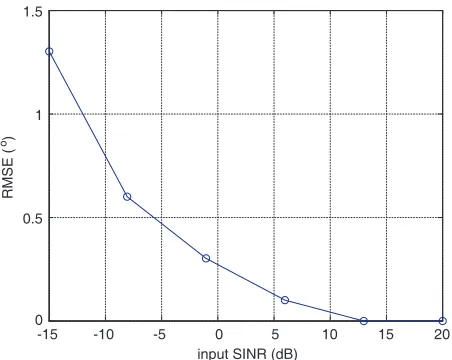
where Y is the number of the Monte Carlo trials, ˆθy the estimated target angle, and θ the real target angle. The results below were from average of 200 independent Monte Carlo experiments. We vary the SINR from−15 dB to 20 dB. It can be clearly observed that using a higher SINR can improve arithmetic precision in Fig. 5, and R-IASLC algorithm performs well at SINR>0 dB.

The resulting plot of output SNR versus look-direction is shown in Fig. 6 for both R-IASLC and IASLC algorithms. From Fig. 6, we can see that the output SNR of R-IASLC is better than IASLC, which is stable at 28 dB. As the look-direction mismatch increases, the IASLC algorithm requires more iterations while the R-IASLC algorithms maintain good convergence. The reason for this is that a large DOA mismatch for IASLC algorithm will result in more interference and noise components in the beamformer output.

To demonstrate the interference suppression capability of R-IASLC algorithms, we plot the normalized beampattern in comparison with IASLC. As shown in Fig. 7, the normalized beampattern of each algorithm can be expressed. The DOA of the desired signal is assumed to be 7◦while the presumed one is 6◦. IASLC algorithm has its main beam pointing to the presumed direction of the desired signal rather than the actual one which will cause the degradation of the output SNR. However, the R-IASLC utilizes iteration algorithm to recover the interference-and-noise suppression capability while maintaining its robustness. It is worth stressing that the R-IASLC method with one cycle iteration or multiple cycle iterations leads to a similar performance in this scenario.

-15 -10 -5 0 5 10 15 20 0

0.5 1 1.5

input SINR (dB)

RMSE ( )

o

Figure 5. RMSE versus input SINR.

4 5 6 7 8 9 10

0 10 20 30 40 50 60 70 80 look-direction (°)

output SNR (dB)

R-IASLC IASLC

Figure 6. Output SNR versus look-direction.

-30 -20 -10 0 10 20 30

-80 -70 -60 -50 -40 -30 -20 -10 0

Normalized Gain (dB)

IASLC R-IASLC

Azimuth Angle ( )o

Figure 7. Normalized gain versus azimuth angle.

-10 -5 0 5 10 15 20

0 10 20 30 40 50 60 70

input SINR (dB)

output SNR (dB)

Optimal IASLC R-IASLC

Figure 8. Output SNR versus input SINR.

The beamformers under comparison are R-IASLC, IASLC as well as optimal SNR. It can be seen from Fig. 8 that the R-IASLC algorithm with cyclic iteration outperforms the IASLC in terms of the output SNR due to its ability to accurately estimate the SV. With the increase of SINR, the performance of R-IASLC is increasingly better than IASLC. The R-IASLC algorithm is almost superimposable with optimality at input SINR>0 dB and obtains about 5 dB superior performance over IASLC when SINR is 0 dB. Therefore, it can be found that R-IASLC offers no mismatch between the actual and presumed SV.

5. CONCLUSION

ACKNOWLEDGMENT

This work was supported in part by the National Natural Science Foundation of China (No. 61771182, No. 61601243, No. 61601167), Aeronautical Science Foundation of China (No. 20162052019), Natural Science Foundation of Jiangsu Province (No. BK20160915) and Science and Technology on Electronic Information Control Laboratory.

REFERENCES

1. Khedekar, S. and M. Mukhopadhyay, “Digital beamforming to reduce antenna side lobes and minimize DOA error,”International Conference on Signal Processing, Communication, Power and

Embedded System, IEEE, 1578–1583, 2017.

2. Quan, G. and G. Li, “A high performance beam forming method based on the secondary combination array,” Advanced Information Management, Communicates, Electronic and

Automation Control Conference, IEEE, 1058–1061, 2017.

3. Shen, M., D. Wu, and D. Zhu, “An ultra-low sidelobe ADBF algorithm for digital array,” Journal

of Electromagnetic Waves and Applications, Vol. 26, Nos. 11–12, 1611–1618, 2012.

4. Cox, H., “Resolving power and sensitivity to mismatch of optimum array processors,” Journal of

the Acoustical Society of America, Vol. 54, No. 3, 771–785, 1973.

5. Krolik, J. L., “The performance of matched-field beamformers with Mediterranean vertical array data,” IEEE Transactions on Signal Processing, Vol. 44, No. 7, 2605–2611, 1996.

6. Lie, J. P., W. Ser, and M. S. S. Chong, “Adaptive uncertainty based iterative robust capon beamformer using steering vector mismatch estimation,” IEEE Transactions on Signal Processing, Vol. 59, No. 6, 4483–4488, 2011.

7. Ke, Y., C. Zheng, R. Peng, et al., “Robust adaptive beamforming using noise reduction preprocessing-based fully automatic diagonal loading and steering vector estimation,”IEEE Access, Vol. 5, No. 99, 12974–12987, 2017.

8. Donelli, M. and P. Febvre, “An inexpensive reconfigurable planar array for Wi-Fi applications,”

Progress In Electromagnetics Research C, Vol. 28, 71–81, 2012.

9. Viani, F., L. Lizzi, M. Donelli, et al., “Exploitation of parasitic smart antennas in wireless sensor networks,”Journal of Electromagnetic Waves and Applications, Vol. 24, No. 7, 993–1003, 2010. 10. Veen, B. D. V. and K. M. Buckley, “Beamforming: A versatile approach to spatial filtering,”IEEE

ASSP Magazine, Vol. 5, No. 2, 4–24, 2002.

11. Yu, K. B. and D. J. Murrow, “Adaptive digital beamforming for angle estimation in jamming,”

IEEE Transactions on Aerospace & Electronic Systems, Vol. 37, No. 2, 508–523, 2002.

12. Liao, B., S. C. Chan, and K. M. Tsui, “Recursive steering vector estimation and adaptive beamforming under uncertainties,”IEEE Transactions on Aerospace&Electronic Systems, Vol. 49, No. 1, 489–501, 2013.

13. Wang, X., J. Xie, Z. He, et al., “A robust generalized sidelobe canceller via steering vector estimation,” Eurasip Journal on Advances in Signal Processing, Vol. 2016, No. 1, 59, 2016.

14. Ke, Y., C. Zheng, R. Peng, et al., “Robust adaptive beamforming using noise reduction preprocessing-based fully automatic diagonal loading and steering vector estimation,”IEEE Access, Vol. 5, No. 99, 12974–12987, 2017.

15. Zhang, T., “Research on robust adaptive beamforming in the presence of array steering vector mismatch,” University of Science and Technology of China, 2014.

16. Shen, F., F. Chen, and J. Song, “Robust adaptive beamforming based on steering vector estimation and covariance matrix reconstruction,”IEEE Communications Letters, Vol. 19, No. 6, 1636–1639, 2015.

17. Li, Y., F. Duan, and J. Jiang, “Robust adaptive beamforming algorithm based on an enhanced diagonal loading method and steering vector estimation,”International Conference on Management

18. Li, J., P. Stoica, and Z. Wang, “On robust Capon beamforming and diagonal loading,” IEEE