A New Analytical Method for Studying Higher Order Modes
of a Two-Wire Transmission Line
Mehdi Gholizadeh* and Farrokh Hojjat Kashani
Abstract—Regarding the increasing application of trahertz (THz) technology, the interest in using two-wire waveguides is getting more and more popular due to their favorable propagation properties. Therefore, a more accurate analysis of these structures is very important. In this paper, a simple analysis of the guided waves in a two-wire waveguide based on Bipolar Coordinate System (BCS) has been investigated. The structure under study is two infinite, perfect electric conductor (PEC) cylinders inz direction, whose axes are positioned at a distance dfrom each other. The solution of TE and TM modes is sought by the aid of electromagnetic formulation, and an analytical expression is proposed for electromagnetic fields and cutoff wavenumbers, which have not been present in any of the previous studies. In this study, for the first time a BCS is used to formulate two-wire waveguide problem, and the validity range of the answer is discussed. The values of the cutoff wavenumbers are calculated for the first few modes of TE and TM, using both the proposed method and Finite Difference Method (FDM). The precise correspondence of the obtained values with the proposed method with those of FDM, along with the high speed and simplicity in implementation, introduces the present method as an appropriate candidate for analyzing transmission lines using parallel cylinders.
1. INTRODUCTION
With the rapid progress of THz technology in recent years, THz waveguides, which are the main components of a THz system, have gained a lot of attention [1]. Several microwave and optical waveguide structures have been used for THz applications such as coplanar strip line, metal pipes, and dielectric fibers. But they all suffer from high loss or high dispersion [2]. It has been demonstrated both experimentally and numerically that two-wire waveguide can be used at THz frequency region successfully with many advantages such as no dispersion, low loss, easy fabrication, and good coupling with common THz sources [3–8]. Besides, there have been lots of work based on this type of waveguide which shows its high importance in microwave and THz frequencies [9–14]. From the point of view of physics, theoretical studies on two-wire waveguide have been based on traditional electrostatic methods, such as image method, distributed parameter theory with equivalent L and C parameters, mapping approach, and approximate field analysis [15–19]. These approaches have been available for solving the problems of its low frequency applications, and they assume only the dominant mode (TEM) on a given structure more often, but for its modern applications of THz or even higher frequencies, a more accurate analysis is necessary. Although there have been some efforts to investigate the higher order modes in two-wire waveguides, they were either unsuccessful or substantially inaccurate [20, 21].
In [20], a method of transforming an eccentric coaxial as well as a double wire line of parallel cylinders into coaxial configuration was used with the aid of the bilinear transformation expressed in terms of mutually inverse points. The cutoff wavelength for TM and TE modes are found from the solution of weighted Helmholtz equation. The weighted Helmholtz equation resulting from the
Received 20 August 2019, Accepted 15 December 2019, Scheduled 27 December 2019 * Corresponding author: Mehdi Gholizadeh (mehdi [email protected]).
transformation was used for finding cutoff wavelengths. This eigenvalue equation was similar to that for a coaxial line except for the presence of a multiplication factor which made the dielectric inhomogeneous. The cutoff wavelengths for TM and TE modes were found from the solution of the weighted Helmholtz equation. The most important point regarding this work is that the numerical data for the two-wire waveguide were not accurate because of the approximations mode in the numerical computation.
In [21], an analytical method was given to study the TEM mode of a two-wire waveguide using a BCS. Considering the finite conductivity of the gold two-wire waveguide in the THz frequency, the equivalent impedance and ohmic loss of two-wire waveguide were calculated. One of the important shortcomings of this paper is the lack of the analysis of TE and TM modes.
Having said that, the features of the dominant mode of the two-wire waveguide can be obtained easily by using conformal mapping. However, for higher-order modes (TE and TM), this method cannot be used. Considering the geometry of the problem and features of the BCS, one can expect that the BCS is very useful in the theoretical investigation of two-wire waveguides. It is noteworthy that Gholizadeh et al. have recently applied a BCS to the analysis of an eccentric coaxial waveguide successfully [22]. Considering the shortcomings in the previous works, this study investigates the higher order modes of a two-wire waveguide. The cutoff wavenumbers of TM and TE modes are determined by enforcing the boundary conditions at the boundaries of the two-wire waveguide, and an analytical expression is proposed for electromagnetic fields. There has been no numerical analysis of the higher order modes of two-wire waveguides. However, in this paper, rather than the proposed analytical solution, the values of cutoff wavenumbers are obtained using FDM in BCS. Zhou et al. have recently applied FDM in BCS to the analysis of an eccentric cable successfully [23]. We have applied the same approach as [23] to calculate the cutoff wavenumbers of TM and TE modes of a two-wire waveguide.
This paper is organized as follows. Section 2 presents the formulation of the problem and its solution. The obtained results are discussed in Section 3. Finally, Section 4 concludes this research.
2. GENERAL ANALYSIS
2.1. Defining the Structure in BCS
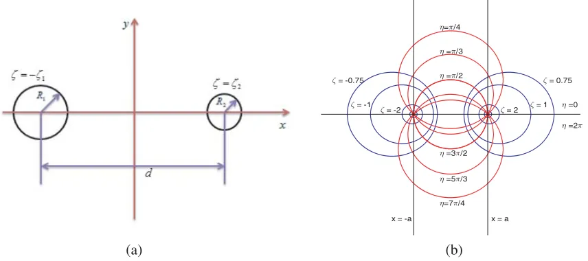
The schematic of a two-wire waveguide is shown in Figure 1(a). It contains two PEC cylinders with radii ofR1 and R2, wheredis the distance between their centers. This type of waveguide can be easily described using BCS (ζ, η, z) as shown in Figure 1(b). The coordinates ζ and η are both dimensionless and change as−∞ ≤ζ ≤ ∞and 0≤η≤2π, respectively. The equations describingζ and η circles are
x = a x = -a
= 0.75 = -0.75
= 1 = -1
= 2 = -2
= /4
= /3
= /2
=7 /4 =5 /3 =3 /2
=2 =0
(a) (b)
as follows:
(x−xc)2+y2 =R2, xc= tanh (a ζ), R= |sinh (a ζ)| (1)
x2+ (y−yc)2=r2, yc = tan (a
η), r =
a
|sin (η)|. (2) where a is an arbitrary positive real number, and 2a shows how far apart the poles of the BCS lie. Moreover, the relation between the BCS and the Cartesian coordinate system is as follows:
x=h1sinh(ζ)
y=h2sin(η)
z=h3z .
(3)
The transversal scale factors are defined as:⎧
⎨ ⎩
h1=h2 = a
cosh (ζ)−cos (η) =h
h3= 1
(4)
From Eqs. (1), (2), and Figure 1, we have:
R1 = a
|sinh(ζ1)|, R2=
a
|sinh(ζ2)| (5)
d = a×(cothζ1+ cothζ2). (6) It is obvious that ζ =−ζ1 and ζ =ζ2 show the surface of the conductors in the BCS.
2.2. The Helmholtz Equation and Boundary Conditions The Helmholtz equation in the BCS can be written as:
∂2ϕ(ζ, η)
∂ζ2 +
∂2ϕ(ζ, η)
∂η2 +
a2k2−kZ2ϕ(ζ, η)
(coshζ−cosη)2 = 0 (7)
and its answer for |ζ| ≥3 is as follows:
ϕ(ζ, η) = (A1sinnη+A2cosnη)×
B1Jn
2aKce−|ζ| +B2Yn
2aKce−|ζ|
(8) where ϕ represents the scalar function that illustrates the longitudinal component of the field (ez in
TM modes and hz in TE modes),kc =k2−k2z and k=ω/c[22].
2.2.1. TM Modes
By employing the Dirichlet boundary condition ϕ(−ζ1, η) = ϕ(ζ2, η) = 0 for TM modes, we have the following equations:
B1Jn2akce−ζ1+B2Yn2akce−ζ1 = 0
B1Jn2akce−ζ2+B2Yn2akce−ζ2 = 0 (9)
By omitting B1 and B2 in Eq. (9), the dispersion equation for TM modes can be obtained as follows:
Jn
2akce−ζ1 Yn2akce−ζ2 −Jn2akce−ζ2 Yn
2akce−ζ1 = 0. (10) Equation (10) can be reformulated as follows:
Jn(bp)Yn(p)−Jn(p)Yn(bp) = 0 (11) whereb=eζ2−ζ1 andp= 2akce−ζ2.
Consequently, the cutoff wavenumbers of TM modes can be derived from the following expression:
kc =
p nm
2a e
ζ2 (12)
2.2.2. TE Modes
By employing the Neumann boundary condition ∂ϕ(ζ1, η)/∂ζ =∂ϕ(ζ2, η)/∂ζ = 0 for TE modes, we have the following equations:
B1Jn 2akce−ζ1+B2Yn2akce−ζ1= 0
B1Jn 2akce−ζ2+B2Yn2akce−ζ2= 0 (13) By omitting B1 and B2 in Eq. (13), the dispersion equation for TE modes can be obtained as follows:
Jn
2akce−ζ1 Yn
2akce−ζ2 −Jn
2akce−ζ2 Yn
2akce−ζ1 = 0. (14) Equation (14) can be reformulated as follows:
Jn bpYnp−Jn pYnbp= 0 (15)
whereb=eζ2−ζ1 andp= 2akce−ζ2.
As a result, the cutoff wavenumbers of TE modes are obtained from the following expression:
kC =
pnm
2a
eζ2 (16)
wherepnm denotes themth root of Eq. (15).
It is clear that the characteristic equations of TE and TM modes (Eqs. (10) and (14), respectively) do not have a unique answer for ζ1 = ζ2. Hence, the condition ζ1 = ζ2 must be considered. In this paper, we have supposedζ1 < ζ2.
2.3. The Solution of the Electric and Magnetic Fields
To obtain an explicit solution for electric and magnetic fields of TE modes in a two-wire waveguide, we have:
H2 = (A1sinnη+A2cosnη)
B1Jn
2aKce−|ξ| +B2Yn
2aKce−|ξ|
e−jβz (17)
Therefore, for electric fields:
Eζ = h(ω−2μεjωμ−β2) ∂
∂η(HZ) =
−jωμ
h(ω2με−β2)(nAcosnη−nBsinnη)
B1Jn
2aKce−|ζ| +B2Yn
2aKce−|ζ|
e−jβz, −ζ1 < ζ < ζ2, 0< η <2π (18)
Eη = h(ω2jωμμε−β2) ∂ ∂ζ(Hz)
= ⎧ ⎪ ⎪ ⎪ ⎪ ⎪ ⎪ ⎪ ⎨ ⎪ ⎪ ⎪ ⎪ ⎪ ⎪ ⎪ ⎩ jωμ
h(ω2με−β2)(A1sinnη+A2cosnη)
−2aKce−ζB1Jn 2aKce−ζ
−2aKce−ζB2Yn2aKce−ζe−jβz, 0< ζ < ζ2, 0< η <2π
jωμ
h(ω2με−β2)(A1sinnη+A2cosnη)
2aKceζB1Jn 2aKceζ
+ 2aKceζB2Yn2aKceζe−jβz, −ζ1 < ζ <0, 0< η <2π
(19)
And for magnetic fields:
Hη = h(ω2−μεjβ−β2) ∂
∂η(Hz) =
−jβ
h(ω2με−β2)(nA1cosnη−nA2sinnη)
B1Jn
2aKce−|ζ| +B2Yn
2aKce−|ζ|
Hζ = h(ω2−μεjβ−β2) ∂ ∂ζ (HZ)
= ⎧ ⎪ ⎪ ⎪ ⎪ ⎪ ⎪ ⎪ ⎨ ⎪ ⎪ ⎪ ⎪ ⎪ ⎪ ⎪ ⎩ −jβ
h(ω2με−β2)(A1sinnη+A2cosnη)
−2aKce−ζB1Jn 2aKce−ζ
−2aKce−ζB2Yn2aKce−ζe−jβz, 0< ζ < ζ2, 0< η <2π
−jβ
h(ω2με−β2)(A1sinnη+A2cosnη)
2aKceζB1Jn 2aKceζ
+2aKceζB2Yn2aKceζe−jβz, −ζ1 < ζ <0, 0< η <2π
(21)
The solution for electric and magnetic fields of TM modes can be obtained similarly.
2.4. FDM
To apply the FDM to the Helmholtz equation, firstly, according to the Taylor series ofϕi,j in the BCS,
we can write:
∂2ϕ
i,j
∂ζ2 =
ϕi+1,j−2ϕi,j+ϕi−1,j
(Δζ)2 +o[(Δζ)
2] (22)
∂2ϕi,j
∂η2 =
ϕi,j+1−2ϕi,j +ϕi,j−1
(Δη)2 +o[(Δη)
2] (23)
Considering Eqs. (7), (22), and (23), we can simply extract the differential form of the Helmholtz equation in the BCS on an orthogonal mesh. Accordingly, using the equation and boundary conditions, a differentiation matrix (X) can be derived to solve the eigenvalue problem:
Xψ =k2cψ=λψ (24)
whereψrepresents the eigenvector of ϕvalues, and λ=kc2 is the required eigenvalue [23]. It is obvious that the entire region of the two-wire waveguide in the BCS can be defined as −ζ1 ≤ ζ ≤ ζ2 and 0 ≤ η ≤ 2π. Hence, rather than the Dirichlet and Neumann boundary conditions (for TM and TE modes, respectively) atζ =−ζ1 andζ =ζ2, the periodic boundary conditions should be applied at the boundaries η= 0 and η= 2π. Also, we can write the parameters of the BCS based on the dimensions of the two-wire waveguide as follows:
a =
(R1+R2)2−d2 ×(R1−R2)2−d2
2d (25)
ζ1 = arcsinh (a/R1) (26)
ζ2 = arcsinh (a/R2) (27)
In order to be convenient for comparison and conversion, we have consideredα=R2/R1 andβ=d/R1. Hence, Equations (25)–(27) can be reformulated as follows:
a =
((1 +α)2−β2)×((1−α)2−β2)
2β (28)
ζ1 = arcsinh(a) (29)
ζ2 = arcsinh(a/α) (30)
The main parameters used in the calculations are summarized in Table 1.
3. NUMERICAL RESULTS AND DISCUSSION
3.1. Evaluation of the Proposed Method
Unlike the introduced parameters ζ1 and ζ2 which are dimensionless, the waveguide has physical dimensions that can be expressed in cm, mm, inch, wavelength, etc. The relationship between ζ1
and ζ2 with physical dimensions of the waveguide is illustrated in Figure 2. Looking at this figure, it is clear that asζ1 increases, the value ofβ increases, too. Obviously, |ζ| ≥3 meansβ ≥20. The values of
Table 1. Main parameters for the calculations using FDM.
Parameters Values
R1 1
R2 α
d β
Range of ζ −ζ1≤ζ ≤ζ2;ζ1 andζ2 calculated from Equations (28)–(30)
Range of η 0≤η ≤2π
Δζ 0.01
Δη 0.01
Figure 2. The values of β against α.
3.2. Investigating the Accuracy of the Proposed Method
The answers of Eqs. (11) and (15) are calculated using MATLAB software, and the values ofpnm and
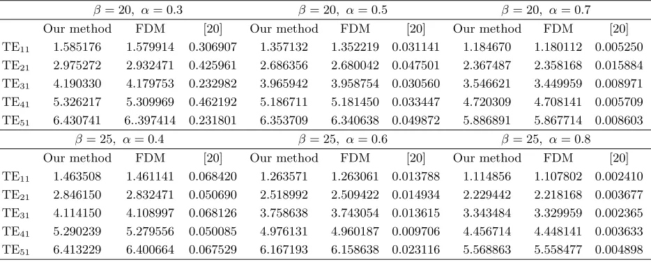
pnm are given in Table 2. Moreover, the cutoff wavenumbers (knm) of TE and TM modes are given
in Table 3 and Table 4, respectively. In these tables, the cutoff wavenumbers are calculated using our analytical method, and the results are compared with those given in [20]. Due to the complexity of the manufacturing process of the structure and the lack of a precise solution for it, we have used the FDM as a reference for the comparison between the two methods. Considering Eqs. (22) and (23), since we chose Δζ = Δη= 0.01 for these calculations, an accuracy of 0.0001 can be achieved.
From the tables we can find that our analytical results coincide with those of the FDM. Our results, both analytical and numerical ones, do not agree with those given in [20]. This is predictable, since in [20] the authors have clearly mentioned that the numerical data for the two-wire waveguide were not accurate because of the approximations mode in the numerical computation. In other words, for solving the weighted Helmholtz equation resulting from the bilinear transformation for the two-wire waveguide, they considered a baseless assumption (w=ρ1ρ2) in order to just obtain a final expression for the cutoff wavenumbers, no matter how the results would be accurate.
Finally, a comparison between the cutoff wavenumber of TE11predicted by our analytical method
Table 2. The values ofpnm andpnm for TE and TM modes, respectively.
p
nm pnm
m m
n 1 2 3 4 5 1 2 3 4 5
β= 20,
α= 0.3
0 1.416120 2.740029 4.079102 5.423540 6.770382 1.328114 2.688640 4.043420 5.396343 6.748453 1 0.475445 1.545459 2.801154 4.118196 5.452276 1.416120 2.740029 4.079102 5.423540 6.770382 2 0.892379 1.886231 2.983809 4.235345 5.538347 1.645554 2.888773 4.184711 5.504586 6.835915 3 1.256814 2.321038 3.284045 4.430800 5.681553 1.952933 3.120060 4.356072 5.637897 6.944302 4 1.597504 2.751540 3.680303 4.706136 5.882286 2.292225 3.413173 4.586522 5.820931 7.094348 5 1.928786 3.149435 4.119634 5.060624 6.142400 2.640368 3.745977 4.867034 6.050206 7.284453
β= 20,
α= 0.5
0 3.208332 6.335964 9.479927 12.628506 15.778995 3.134891 6.297118 9.453717 12.608763 15.763169 1 0.678140 3.294034 6.376742 9.506739 12.648508 3.208332 6.335964 9.479927 12.628506 15.778995 2 1.342334 3.542342 6.497992 9.586832 12.708365 3.418422 6.451185 9.558174 12.687576 15.826395 3 1.981725 3.930427 6.696694 9.719213 12.807638 3.740117 6.639044 9.687341 12.785502 15.905127 4 2.591726 4.427961 6.968510 9.902333 12.945620 4.144478 6.893925 9.865658 12.921522 16.014796 5 3.174859 5.002306 7.308540 10.134236 13.121377 4.606183 7.209022 10.090826 13.094616 16.154869
Table 3. The cutoff wavenumbers (knm) for TE modes. Comparison with [20] and the results of the FDM.
β= 20, α= 0.3 β= 20, α= 0.5 β= 20, α= 0.7
Our method FDM [20] Our method FDM [20] Our method FDM [20]
TE11 1.585176 1.579914 0.306907 1.357132 1.352219 0.031141 1.184670 1.180112 0.005250
TE21 2.975272 2.932471 0.425961 2.686356 2.680042 0.047501 2.367487 2.358168 0.015884
TE31 4.190330 4.179753 0.232982 3.965942 3.958754 0.030560 3.546621 3.449959 0.008971
TE41 5.326217 5.309969 0.462192 5.186711 5.181450 0.033447 4.720309 4.708141 0.005709
TE51 6.430741 6..397414 0.231801 6.353709 6.340638 0.049872 5.886891 5.867714 0.008603
β= 25, α= 0.4 β= 25, α= 0.6 β= 25, α= 0.8
Our method FDM [20] Our method FDM [20] Our method FDM [20]
TE11 1.463508 1.461141 0.068420 1.263571 1.263061 0.013788 1.114856 1.107802 0.002410
TE21 2.846150 2.832471 0.050690 2.518992 2.509422 0.014934 2.229442 2.218168 0.003677
TE31 4.114150 4.108997 0.068126 3.758638 3.743054 0.013615 3.343484 3.329959 0.002365
TE41 5.290239 5.279556 0.050085 4.976131 4.960187 0.009706 4.456714 4.448141 0.003633
TE51 6.413229 6.400664 0.067529 6.167193 6.158638 0.023116 5.568863 5.558477 0.004898
3.3. Investigating the CPU Computation Time of Our Method and the FDM
In Table 5, the CPU computation times of our analytical method and the FDM are compared. The time is measured using the Tic-Toc functions in MATLAB software. For this measurement, a personal computer with the following specifications is used:
• CPU: Core i5, 2.5 GHz.
• RAM: 4 GB
Table 4. The cutoff wavenumbers (knm) for TM modes. Comparison with [20] and the results of FDM.
β= 20, α= 0.3 β= 20, α= 0.5 β= 20, α= 0.7
Our method FDM [20] Our method FDM [20] Our method FDM [20]
TM1 4.428049 4.419144 0.309592 6.273724 6.265761 0.032054 10.512977 10.509137 0.019137
TM11 4.721467 4.716471 0.077735 6.420697 6.419422 0.047687 10.579667 10.564593 0.015933
TM21 5.486420 5.479753 0.306804 6.841142 6.838305 0.031000 10.777206 10.770177 0.005177
TM31 6.511249 6.498556 0.462487 7.484935 7.471189 0.047314 11.098452 11.015836 0.015836
TM41 7.642479 7.630664 0.232542 8.294166 8.280638 0.050324 11.532820 11.518840 0.008840
β= 20, α= 0.4 β= 20, α= 0.6 β= 20, α= 0.8
Our method FDM [20] Our method FDM [20] Our method FDM [20]
TM1 5.196193 5.188441 0.041146 7.853183 7.848336 0.014108 15.759716 15.750012 0.002481
TM11 5.404252 5.398924 0.064944 7.954753 7.945631 0.010197 15.799131 15.788168 0.003691
TM21 5.979003 5.965097 0.068348 8.251627 8.245937 0.013746 15.916786 15.909959 0.002399
TM31 6.813000 6.806675 0.050491 8.722939 8.714211 0.014855 16.110951 16.100981 0.003662
TM41 7.803645 7.789206 0.067904 9.340856 9.329724 0.013482 16.378881 16.364771 0.004925
Table 5. The CPU computation time comparison of using our analytical method and FDM.
β= 20, α= 0.3 β= 20, α= 0.5
Our analytical method FDM Our analytical method FDM
TE11 0.014512 5.765457 0.038425 8. 357141
TE21 0.018874 5.835261 0.063325 8.397877
TE31 0.023345 5.884356 0.081732 8.463256
TE41 0.031149 5.953547 0.095671 8.537683
TE51 0.038892 5.995379 0.117438 8.638943
Average time 0.025354 5.886800 0.079318 8.478980
Figure 3. The cutoff wavenumber of TE11, comparison with its value using FDM at different values
4. CONCLUSIONS
The problem has been investigated in a fully analytical manner, and analytical expressions have been obtained for the electric and magnetic field functions and cutoff wavenumbers. The presented method gives accurate results for β ≥ 20. An excellent agreement between the calculated cutoff wavenumbers and those obtained by the FDM is observed. The combination of accuracy, analyticity, and ease of implementation makes this method an appropriate option for analysis of transmission lines using parallel cylinders. Future steps of this study can fall into the following subjects: analysis of circular waveguides which are loaded with eccentric dielectric materials, analysis of dielectric coating on the inner conductor of an eccentric coaxial waveguide, and analysis of scattering of electromagnetic waves from an eccentrically coated circular PEC cylinder.
REFERENCES
1. Mbonye, M. K., V. Astley, W. L. Chan, J. A. Deibel, and D. M. Mittleman, “A THz dual wire waveguide,” Conf. Lasers Electro-Optics (p. CThLL1). Opt. Soc. Am., 2007.
2. Zhong, R. B., M. Hu, Y. Zhang, and S. G. Liu, “Theoretical study on dual-wire waveguide,”
Infrared, Millimeter, THz Waves, 2009. IRMMW-THz 2009. 34th Int. Conf. (1-2). IEEE, 2009, DOI: 10.1109/ICIMW.2009.5324777.
3. Mbonye, M., R. Mendis, and D. Mittleman, “A THz two-wire waveguide with low bending loss,”
Appl. Phys. Lett., Vol. 95, 233506, 2009.
4. Pahlevaninezhad, H. and T. E. Darcie, “Coupling of THz waves to a two-wire waveguide,” Opt. Express, Vol. 18, No. 22, 22614–22624, 2010.
5. Pahlevaninezhad, H., T. Darcie, and B. Heshmat, “Two-wire waveguide for THz,” Opt. Express, Vol. 18, 7415–7420, 2010.
6. Dickason, J. and K. W. Goosen, “Loss analysis for a two wire optical waveguide for chip-to-chip communication,” Opt. Express, Vol. 21, 5226–5232, 2013.
7. Markov, A. and M. Skorobogatiy, “Two-wire THz fibers with porous dielectric support,” Opt. Express, Vol. 21, No. 10, 12728-43, May 2013.
8. Gao, H., Q. Cao, D. Teng, M. Zhu, and K. Wang, “Perturbative solution for THz two-wire metallic waveguides with different radii,”Opt. Express, Vol. 23, No. 21, 27457-73, Oct. 19, 2015.
9. Hinds, E. A., C. J. Vale, and M. G. Boshier, “Two-wire waveguide and interferometer for cold atoms,” Physical Review Letters, Vol. 86, No. 8, 1462, Feb. 19, 2001.
10. Markov, A., H. Guerboukha, and M. Skorobogatiy, “Hybrid metal wire-dielectric THz waveguides: Challenges and opportunities,”JOSA B, Vol. 31, No. 11, 2587–600, Nov. 1, 2014.
11. Teng, D., Q. Cao, S. Li, and H. Gao, “Tapered dual elliptical plasmon waveguides as highly efficient THz connectors between approximate plate waveguides and two-wire waveguides,” JOSA A, Vol. 31, No. 2, 268-73, Feb. 1, 2014.
12. Markov, A., G. Yan, and M. Skorobogatiy, “Low-loss THz waveguide Bragg grating using a two-wire waveguide and a paper grating,”Infrared, Millimeter, THz waves (IRMMW-THz), 2014 39th Int. Conf. on. IEEE, Vol. 38, No. 16, 3089–3092, 2014.
13. Mridha, M. K., et al., “Active THz two-wire waveguides,” Opt. Express, Vol. 22, No. 19, 22340, 2014.
14. Zha, J., G. J. Kim, and T. I. Jeon, “Enhanced THz guiding properties of curved two-wire lines,”
Opt. Express, Vol. 24, No. 6, 6136-44, Mar. 21, 2016. 15. Schelkunoff, A. S.,Electromagnetic-Waves, 1943.
16. Lee, K. S. H., “Two parallel terminated conductors in external fields,”IEEE Trans. Electromagn. Compat., Vol. 20, No. 2, 288–296, 1978.
18. Paul, C. R., Analysis of Multiconductor Transmission Lines, 2nd Edition, John Wiley & Sons, 2008.
19. Tannouri, P., M. Peccianti, P. L. Lavertu, F. Vidal, and R. Morandotti, “Quasi-TEM mode propagation in twin-wire THz waveguides,”Chin. Opt. Lett., Vol. 09, 110013, 2011.
20. Das, B. N. and O. J. Vargheese, “Analysis of dominant and higher order modes for transmission lines using parallel cylinders,” IEEE Trans. Microw. Theory Tech., Vol. 42, No. 4, 681–683, 1994. 21. Zhong, R., J. Zhou, W. Liu, and S. Liu, “Theoretical investigation of a THz transmission line in
bipolar coordinate system,”Sci. China Inf. Sci., Vol. 55, No. 1, 35–42, Jan. 2012.
22. Gholizadeh, M., M. Baharian, and F. H. Kashani, “A simple analysis for obtaining cutoff wavenumbers of an eccentric circular metallic waveguide in bipolar coordinate system,”IEEE Trans. Microw. Theory Tech., Vol. 67, No. 3, 837–844, Mar. 2019.

![Table 4. The cutoff wavenumbers (knm) for TM modes. Comparison with [20] and the results of FDM.](https://thumb-us.123doks.com/thumbv2/123dok_us/1965139.1259158/8.612.167.436.459.701/table-cuto-wavenumbers-knm-modes-comparison-results-fdm.webp)
