Spatial and Polarization Angle Estimation of Mixed-Targets
in MIMO Radar
Srinivasarao Chintagunta1, * and Palanisamy Ponnusamy2
Abstract—This paper proposes an approach for estimating the spatial and polarization angles of mixed-targets in bistatic MIMO radar. Mixed-targets mean the combination of uncorrelated, partially correlated, and groups of coherent targets. The approach resolves rank deficiency of received signal covariance matrix and then exploits the ESPRIT-based method for estimating the angles of direction-of-departure (DOD) and direction-of-arrival (DOA). This paper also presents an analytical review and necessary conditions for resolving the rank deficiency under various scenarios of the MIMO radar. Simulation results show the effectiveness of the proposed approach.
1. INTRODUCTION
Multiple-input multiple-output (MIMO) radar has been receiving much attention for localization of the targets over the conventional phased array radar [1]. For localization of the targets, direction estimation is a key issue and has found many investigations in the literature [2–9]. Majority of these investigations focus on the estimation of direction-of-departure (DOD) and direction-of-arrival (DOA) of uncorrelated targets [2–7] and coherent targets [8, 9]. Two-dimensional (2D) DOD and 2D-DOA estimation have also been investigated for the case of uncorrelated targets [10–12]. 2D means azimuth and elevation angles of a target. The 2D DOD/DOA estimation is important specifically when the targets are resolvable in azimuth angles but not resolvable in elevation angles, and vice-versa.
Moreover, in a stringent scenario where the targets are closely spaced and cannot be resolvable with spatial angles, the polarization estimation may be required for localizing and distinguishing the targets. Though the estimation of signal parameters via rotational invariance technique (ESPRIT) based method in [12] estimates both spatial and polarization angles, estimation performance is shown only for the spatial angles. However, this ESPRIT-based method fails under the coherent target scenario due to the rank deficiency of received signal covariance matrix. In practice, the received signals are coherent or partially correlated or may be a combination of coherent and partially correlated [13–15]. Therefore, in this paper, we formulate a model for mixed targets which are the combination of uncorrelated, partially correlated, and groups of coherent targets, and estimate both spatial and polarization angles. The methodology of this paper resolves the rank deficiency of mixed targets using spatial smoothing and then estimates the angles employing the ESPRIT-based method [12]. This paper also presents an analytical discussion and necessary conditions of the smoothing for decorrelating the mixed targets under different scenarios of the MIMO radar.
Notation: Vectors and matrices are represented by lowercase and uppercase bold characters,
respectively. (·)T denotes the transpose, and (·)H indicates the conjugate-transpose. Symbols ⊗, , and ⊕ denote the Kronecker product, Khatri-Rao product, and Hadamard product, respectively. In,
0m×n, and 0n denoten×nidentity matrix,m×nzeros matrix, andn×nzeros matrix, respectively. In
particular, diag{·}and blkdiag{·}represent the diagonal matrix and block diagonal matrix, respectively. [J]k,k selects the entry in the kth row andkth column of matrixJ.
Received 17 April 2019, Accepted 5 June 2019, Scheduled 20 June 2019 * Corresponding author: Srinivasarao Chintagunta ([email protected]).
2. SIGNAL MODEL
Consider a bistatic MIMO radar that comprises uniform linear arrays of M electromagnetic vector sensors (EVSs) and N EVSs at the transmitter and receiver, respectively. Each EVS consists of three orthogonally oriented electric-dipoles and three orthogonally oriented magnetic-loops. The inter-sensor spacing of the transmit array isdt, and the receive array isdr. Suppose that there areK targets present
in the same range cell. Then, deploying the arrays along the y-axis, steering vectors of the transmit array at and receive arrayar towards thekth target direction can be expressed as
atk =btk(θtk,φtk)⊗ctk(θtk,φtk,γtk,ηtk)
ark =brk(θrk,φrk)⊗crk(θrk,φrk,γrk,ηrk)
(1)
where btk = [1,αk,. . .,α M−1
k ]T in which αk = e−j2πdtsinθtksinφtk/λ with λ being the wavelength, and
brk = [1,βk,. . .,β N−1
k ]
T in whichβ
k=e−j2πdrsinθrksinφrk/λ. ct
k/crk denotes the spatial response vector
of the transmitting/ receiving EVS. The subscript tk/rk indicates that the concerning parameter or
vector belonging to the transmitter/receiver associated with the kth target. Thus, the spatial response vector ci,i= tk, rk, of an EVS can be expressed as
ci=F(θi,φi)g(γi,ηi) =
⎡ ⎢ ⎢ ⎢ ⎢ ⎢ ⎣
cosθicosφi −sinφi
cosθisinφi cosφi −sinθi 0 −sinφi −cosθicosφi
cosφi −cosθisinφi
0 sinθi
⎤ ⎥ ⎥ ⎥ ⎥ ⎥ ⎦
sinγiejηi
cosγi (2)
where φi ∈ [0, 2π), θi ∈ [0,π), γi ∈ [0,π/2), and ηi ∈ [−π,π) respectively denote the azimuth angle,
elevation angle, auxiliary polarization angle, and the polarization phase difference of the concerning target (i.e., i= tk, rk).
Assume that the elements of the transmit-array transmit orthogonal coded vector signals V = [v1,1,. . .,v1,6,. . .,vM,1,. . .,vM,6]T, wherevm,idenotes theP×1 coded vector signal by theith element
of themth EVS. The transmitted signals are reflected at K far-field targets. Then the received signal at thelth snapshot can be expressed as
X(l) =
K
k=1
arksk(l)a T
tkV+W(l) (3)
In practice, vectorization of the output of matched filters matched to the transmission signal is used for processing the signal [5, 6]. The output of the matched filter bank is represented by Xout(l) =
X(l)VH/√P. Then the vectorization of Xout(l) can be expressed as [12]
y(l) = vec(Xout(l)) =
K
k=1
(atk⊗ark) √
P sk(l) +z(l) =As(l) +z(l) (4)
whereA= [at1⊗ar1,. . .,atK ⊗arK],s(l) = [ √
P s1(l),. . .,
√
P sK(l)]T denotes the reflectivity vector at
output of the matched filters, andz(l) = √1
Pvec(W(l)V
H) is the output noise vector.
3. PROPOSED APPROACH
3.1. Problem Formulation
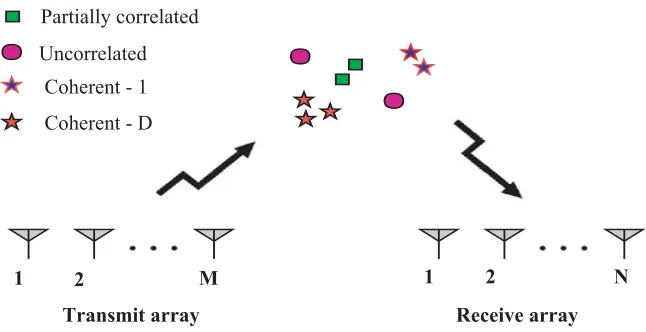
In a practical scenario, as the model shown in Fig. 1, the nonzero reflectivities {sk(l)}Kk=1 are the
combination of uncorrelated, partially correlated, and groups of coherent. Without loss of generality, assume that the firstKutargets (in fact, target reflectivities) are uncorrelated, nextKptargets partially
correlated, and the remaining areDclusters of Kc=
D
1 2 M 1 N
Transmit array Receive array
Coherent - 1 Coherent - D Partially correlated Uncorrelated
2
Figure 1. Model map of the scenario considered in problem formulation.
are coherent and uncorrelated with the targets in other clusters as well asKu uncorrelated targets and Kp partially correlated targets. Under this scenario, the signal model in Eq. (4) can be written as
y(l) =Ausu(l) +Apsp(l) +Acsc(l) +z(l) = [Au, Ap, Ac]
s
u(l)
sp(l)
sc(l)
+z(l) (5)
whereAu= [at1⊗ar1,. . .,atKu ⊗arKu] represents the steering matrix of all uncorrelated targets;Ap =
[atKu+1⊗arKu+1,. . .,atKu+Kp ⊗arKu+Kp] denotes the steering matrix of all partially correlated targets,
Ac = [Ac1,. . .,AcD] in which Acd = [atd,1⊗ard,1,. . .,atd,Qd ⊗ard,Qd], d= 1,. . .,D, being the steering
matrix concerning with all coherent targets in thedth cluster;su(l) = [
√
P s1(l),. . .,
√
P sKu(l)]T denotes
the reflectivity vector of uncorrelated targets; sp(l) = [
√
P sKu+1(l),. . .,
√
P sKu+Kp(l)]T represents the
reflectivity vector of all partially correlated targets; and sc(l) = [sTKu+Kp+1(l),. . .,sTKu+Kp+D(l)]T in
which sKu+Kp+d(l) being the reflectivity vector of all coherent targets in dth cluster. Further, the
coherent reflectivity vectorsKu+Kp+d(l) can be decomposed assKu+Kp+d(l) = √
P sKu+Kp+d(l)ρd, where
sKu+Kp+d(l) is the common reflectivity of the dth cluster, and ρd = [ρd,1,. . .,ρd,Qd]
T denotes the
complex coefficient vector of dth cluster. The coefficients in ρd represent the magnitude and phase
relationship of Qd coherent targets in the dth cluster.
Therefore, the covariance matrix of the signaly(l) in Eq. (5) is given by
Ry =E
y(l)y(l)H=ARsAH+Rz (6)
whereA= [Au, Ap, Ac],Rs = blkdiag{Ru,Rp,Rc}in whichRu= diag{σ12,. . .,σK2u}is the covariance
matrix of su(l); Rp is the covariance matrix of sp(l); Rc = blkdiag{Rc1,. . .,RcD} is the covariance
matrix ofsc(l);Rcd(d= 1,. . .,D) denotes the covariance ofsKu+Kp+d(l); andRzis the noise covariance
matrix.
For mixed targets, the rank ofRsis less than the number of targets present, and thus rank(Ry)< K
under the noise-free condition. Consequently, the ESPRIT-based method in [12] fails to resolve the targets as the angle estimates of DODs and DOAs are inaccurate.
3.2. Construction of a Full-Rank Covariance Matrix
The spatial smoothing of the MIMO radar divides the transmit array and receive array into Pt and Pr numbers of uniformly overlapped subarrays, respectively. Each transmitting subarray comprises Mt EVSs, and each receiving subarray has Nr EVSs. Considering the maximum overlapping of the
subarrays, we can obtain Pt = M −Mt + 1 and Pr = N −Nr + 1 numbers of subarrays. In fact,
the mth (m = 1,. . .,Pt) transmitting subarray and the nth (n = 1,. . .,Pr) receiving subarray be
denoted withR[ym,n]∈C36MtNr×36MtNr. Then the subarrays covariance matricesR[ym,n]can be obtained
from Ry as R[ym,n] = (J1 ⊗J2)Ry(J1 ⊗J2)T, where J1 = [06Mt×6(m−1) | I6Mt | 06Mt×6(Pt−m)] and
J2 = [06Nr×6(n−1) |I6Nr | 06Nr×6(Pr−n)]. Now, as the conventional forward-only spatial smoothing, the
smoothed covariance matrixRfoy can be expressed as
Rfoy = 1
PtPr
Pt
m=1
Pr
n=1
R[ym,n]=AR˜ fos A˜H+Rfoz (7)
whereA˜ = [˜at1 ⊗˜ar1,. . .,˜atK ⊗˜arK] in which˜atk and ˜ark,∀k= 1,. . .,K, represent the first 6Mt and
the first 6Nr rows of atk and ark, respectively; the matrix Rfos , given in Eq. (8), is the modified and
smoothed version ofRs in which the modification is performed by the joint transmitting and receiving
array spatial phase-shift factors; andRfoz is the smoothed noise covariance matrix. The matrix Rfos can be expressed as
Rfos = 1
PtPr
Pt
m=1
Pr
n=1
Φmt −1Φnr−1RsΦ1t−mΦ1r−n (8)
whereΦt= blkdiag{Φtu,Φtp,Φtc}in whichΦtu= diag{α1,. . .,αKu},Φtp= diag{αKu+1,. . .,αKu+Kp},
and Φtc = blkdiag{Φtc1,. . .,ΦtcD} with Φtcd = diag{αd,1,. . .,αd,Qd},∀ d = 1,. . .,D; and Φr =
blkdiag{Φru,Φrp,Φrc} in which Φru = diag{β1,. . .,βKu}, Φrp = diag{βKu+1,. . .,βKu+Kp}, and
Φrc = blkdiag{Φrc1,. . .,ΦrcD} with Φrcd = diag{βd,1,. . .,βd,Qd},∀ d = 1,. . .,D. The factors αk (k = 1,. . .,Ku), αKu+p (p = 1,. . .,Kp) and αd,q (q = 1,. . .,Qd) denote the spatial phase-shift
between the consecutive subarrays of the transmit array associated with the kth uncorrelated target, the pth partially correlated target, and the qth coherent target in the dth cluster, respectively. Se-quentially, βk,βKu+p, andβd,q are the spatial phase-shift factors of the consecutive subarrays of receive
array.
The matrixRfos in Eq. (8) is now full-rank, i.e., rank(Rfos ) =K, subject to satisfying the following conditions:
Condition 1: The coherent targets within the cluster should consist of either different azimuth angles or different elevation angles associated with both the DODs and DOAs.
Condition 2: The total number of subarrays should be greater than the maximum of the targets number in all clusters, i.e.,PtPr≥Q, where Q= max(Q1,. . .,QD).
3.3. Validation of the Full-Rank of Smoothed Covariance Matrix
For uncorrelated or partially correlated targets, the reflectivity covariance matrix has a full-rank, i.e., rank(Ru) =Ku and rank(Rp) =Kp. Thus, the rank deficiency of Rs has occurred due to the weaker
rank of Rc, i.e., rank(Rc) = D < Kc, where Kc =
D
d=1Qd with Qd≥2,∀ d= 1,. . .,D. Besides, the
smoothing does not reduce the rank ofRu andRp. Therefore, the task is now to show that the rank of
Rfoc isKc.
Upon substitutingRs = blkdiag{Ru,Rp,Rc} in Eq. (8), the segment with only the termRc can
be expressed as
Rfoc = 1
PtPr
Pt
m=1
Pr
n=1
Φmtc−1Φnrc−1RcΦ1tc−mΦ1rc−n (9)
Further, from the definition ofRc= blkdiag{Rc1,. . .,RcD}, Eq. (9) can be simplified as
Rfoc = blkdiag
Rfoc1,. . .,RfocD
(10)
where
Rfocd= 1
PtPr
Pt
m=1
Pr
n=1
Φtcmd−1Φrcn−d1RcdΦ1tc−dmΦ
1−n
Equation (10) shows that rank(Rfoc) = Kc, if, and only if, the rank(Rfocd) =Qd, ∀ d= 1,. . .,D. Now,
upon substituting Rcd =σ
2
Ku+Kp+dρdρHd in Eq. (11), Rfocd can be expressed as
Rfoc
d =
σK2u+Kp+d
PtPr
Pt
m=1
Pr
n=1
Φmtc−1
d Φ
n−1 rcd ρdρ
H
dΦ1tc−dmΦ
1−n
rcd = Λd
˜
BdΨdB˜HdΛdH, ∀ d= 1,. . .,D, (12)
where Λd diag{ρd,1,. . .,ρd,Qd} ∈ C
Qd×Qd, Ψ
d diag{
σ2Ku+Kp+d PtPr ,. . .,
σ2Ku+Kp+d PtPr } ∈ R
PtPr×PtPr, and
˜
Bd = (B˜td B˜rd)
T ∈ CQd×PtPr in which B˜t
d = [˜bt(θtd,1,φtd,1),. . .,b˜t(θtd,Qd,φtd,Qd)] ∈ C Pt×Qd
and B˜rd = [˜br(θrd,1,φrd,1),. . .,b˜r(θrd,Qd,φrd,Qd)] ∈ C
Pr×Qd. Besides, the vectors b˜
t(θtd,k,φtd,k) and
˜
br(θrd,k,φrd,k) denote the first Pt rows of bt(θtd,k,φtd,k), and the first Pr rows of br(θrd,k,φrd,k),
respectively. Clearly, from the above definition, rank(Λd) = Qd and rank(Ψd) = PtPr provided that ρd,k= 0, ∀ k= 1,. . .,Qd andσK2u+Kp+d= 0, ∀d= 1,. . .,D, respectively.
The matrices B˜td and B˜rd comprise the Vandermonde structures. Thus, if satisfying either θtd,k = θtd,p or φtd,k = φtd,p, ∀ k = p, k,p ∈ (1,. . .,Qd), then the rank(B˜td) = min(Pt,Qd).
Likewise, if satisfying either θrd,k = θrd,p or φrd,k = φrd,p, ∀ k = p, k,p ∈ (1,. . .,Qd), then the
rank(B˜rd) = min(Pr,Qd). Besides, the DODs and DOAs are different because the system model
is bistatic MIMO radar, i.e., θtd,k = θrd,k or φtd,k = φrd,k, ∀ k = 1,. . .,Qd. Thus, the matrix
˜
Bd consists of 2Qd generators of B˜td and B˜rd. This condition assures the rank of B˜d is full, i.e.,
rank(B˜d) = min(PtPr,Qd). This holds forCondition 1.
From the matrix form of Rfocd in Eq. (12), the rank of Rfocd is Qd when PtPr ≥ Qd. Consequently,
from Eq. (10), rank(Rfoc) = Kc can be obtained intuitively when we choose PtPr ≥ Q, where Q= max(Q1,. . .,QD) with any choice of Pt≥1 andPr≥1. This holds forCondition 2.
In the above-said conditions, the first condition can be relaxed, but it restricts more on the minimum subarrays required (i.e., second condition) to attain the full-rank. These are described as the following notes:
Note 1: In the case of monostatic MIMO radar (i.e., DODs and DOAs are identical), the matrixB˜d
contains onlyPt+Pr−1 different elements in each row. Thus, rank(B˜d) is limited by min(Pt+Pr−1,Qd),
and rank(Rfoc ) =Kc is achieved only whenPt+Pr−1≥Q.
Note 2: If θtd,k =θtd,p and φtd,k = φtd,p with satisfying either θrd,k =θrd,p or φrd,k =φrd,p ∀ k = p, k,p= 1,. . .,Qdand∀d= 1,. . .,D, then the rank ofB˜d= min(Pr,Qd) which is due to rank(B˜td) = 1
and rank(B˜rd) = min(Pr,Qd). Thus, the rank(R
fo
c) = Kc is fulfilled only when Pr ≥Q irrespective of
any Pt.
Note 3: If θrd,k = θrd,p and φrd,k = φrd,p with satisfying either θtd,k = θtd,p or φtd,k = φtd,p ∀ k = p, k,p = 1,. . .,Qd and ∀ d = 1,. . .,D, then the rank of B˜d = min(Pt,Qd) as the
rank(B˜td) = min(Pt,Qd) and rank(B˜rd) = 1. Thus, rank(R
fo
c ) = Kc is attained only when Pt ≥ Q
irrespective of anyPr.
3.4. Estimation of the Spatial and Polarization Angles
After obtaining the smoothed covariance matrix as described in Section: 3.2, angles are estimated using the ESPRIT-based method [12]. The algorithmic steps of the overall approach are as follows:
(i) Compute the snapshot covariance matrix ofy(l) in (5) usingLsnapshots asRˆy= L1
L
l=1y(l)yH(l).
(ii) Compute the smoothed covariance matrixRfoy by Eq. (7).
(iii) EigendecomposeRfoy for obtaining the signal-subspace Es and the noise-subspace En.
(iv) PartitionEsintoEt=J3EsandEr=J4Es, whereJ3 =I6Mt⊗eTq1,q1∈(1,. . ., 6Nr) in whicheq1 is
theq1th column ofI6Nr, andJ4 = [06Nr×6q2Nr |I6Nr |06Nr×(36MtNr−6(q2+1)Nr)],q2∈(0,. . ., 6Mt−1).
where J5 = [I6(Mt−1) | 06(Mt−1),6], J6 = [06(Mt−1),6 | I6(Mt−1)], J7 = [I6(Nr−1) | 06(Nr−1),6], and
J8= [06(Nr−1),6 |I6(Nr−1)].
(v) Estimate {ctk} K
k=1 as [ˆct1,. . .,ˆctK] =
1
Mt
Mt
i=1(E˜tiT−
1
cr Λ1t−i), where Λtand Tcrare the eigenvalues
and the right-eigenvectors of {(EHt1EHt1)−1EHt1Et2}, respectively, and E˜ti represents (6i-5)th row to
(6i)th row ofEt.
(vi) Compute the cross product between the first three and the conjugate of remaining three components ofˆctk for each k= 1,. . .,K, which obtains (ˆutk, ˆvtk, ˆwtk) = (sin ˆθtkcos ˆφtk, sin ˆθtksin ˆφtk, cos ˆθtk).
Thus, ˆθtk = sin−1(
ˆ
u2t k+ ˆv
2
tk) and ˆφtk = tan−1( ˆ
vtk ˆ
utk), k= 1,. . .,K.
(vii) From Eq. (2), ˆgk
ˆ
g1k
ˆ
g2k
= (FH(ˆθtk, ˆφtk)F(ˆθtk, ˆφtk))−
1FH(ˆθ
tk, ˆφtk)ˆctk. Thus, ˆγtk = tan−
1(|gˆ1k
ˆ
g2k|)
and ˆηtk =∠(
ˆ
g1k
ˆ
g2k), k= 1,. . .,K.
(viii) For estimating θrk, φrk, γrk and ηrk, repeat the steps v, vi, and vii with Er, Er1 and Er2 instead
Et,Et1 andEt2.
(ix) Let ˆΦt and ˆΦr denote the parameters {θˆt, ˆφt, ˆγt, ˆηt} and {θˆr, ˆφr, ˆγr, ˆηr}, respectively. Thus, thekth
column ofA˜ can be denoted as˜a( ˆΦtk, ˆΦrk) =˜atk( ˆΦtk)⊗˜ark( ˆΦrk), k= 1,. . .,K. From step vi and
step vii, the parameters within ˆΦt of a particular target are paired automatically. Likewise, the
parameters within ˆΦr of a particular target are also automatically paired. Then, based on the fact
that the columns ofA˜ are orthogonal to the columns ofEn, pairing between ˆΦtand ˆΦrof a particular
target can be obtained by findingf( ˆΦtk, ˆΦrp)˜a H( ˆΦ
tk, ˆΦrp)EnE H
n˜a( ˆΦtk, ˆΦrp), k,p= 1,. . .,K, and
selecting the minimum value concerning ˆΦrp for each ˆΦtk.
3.5. Complexity Analysis
Computational complexity of the proposed approach depends mainly on the computation of step i, step ii, step iii, DODs estimation (step v–step vii), DOAs estimation, and the pairing between DODs and DOAs (step ix). The complexity of step i, step ii, and step iii is O{(6M)2(6N)2L},
O{(6Mt)2(6Nr)2}, and O{(6Mt)3(6Nr)3}, respectively. The DODs estimation requires the complexity
ofO{2K26(Mt−1) + 3K3+ 7MtK2}for step v,O{6K}for step vi, andO{48K} for step vii. Likewise,
DOAs requires the complexity of O{2K26(Nr −1) + 3K3+ 7NrK2+ 54K}. Finally, pairing between
the DODs and DOAs requiresO{(36MtNr(36MtNr−K) + (36MtNr−K))K2}.
4. CRAMER-RAO LOWER BOUND
As described the signal model in Section 2, according to [16], the Cramer-Rao bound (CRB) of all parameters to be estimated can be obtained as
J= σ
2
z
2L
Re
EHΠ⊥AE⊕R†sT
−1
(13)
where σz2 is the noise variance, E = [{∂ak
∂θtk}Kk=1,{
∂ak
∂φtk}Kk=1,. . .,{
∂ak
∂ηrk}Kk=1], Π⊥A = I36M N −
A(AHA)−1AH, and Rs† = 18⊗Rs in which 18 is 8×8 unit matrix. The root CRB of particular
parameterψ∈(θt,φt,γt,ηt,θr,φr,γr,ηr) can be obtained as
CRB(ψ) =
1
K
K
k=p+1
[J]k,k (14)
5. SIMULATION RESULTS
This section presents the Monte-Carlo simulations to examine the effectiveness of the proposed approach. For all simulations, we considerM =N = 10 EVSs with spacing dt=dr=λ/2,Pt=Pr= 6 subarrays
for performing the smoothing, Hadamard codes of length P = 128 for transmission of the orthogonal waveforms, q1 = 2 in J3 and q2 = 1 in J4 for partitioning Es, and the noise is complex Gaussian with
zero mean. All simulations are executed over Mc= 500 Monte-Carlo runs.
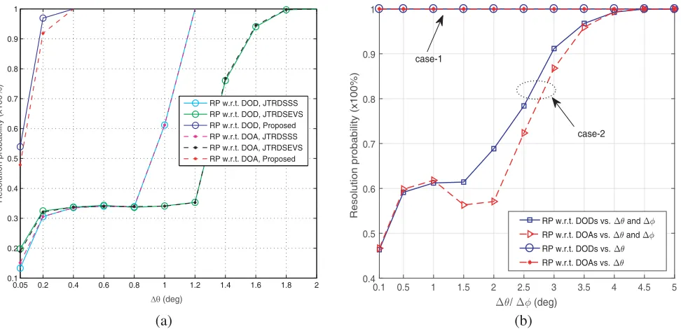
In the first simulation, shown in Fig. 2, we describe the advantage of both spatial and polarization angle estimation by evaluating the resolution probability (RP). The RP for resolving a target concerning with the DODs/DOAs is computed statistically from the successful trials, which accounts when the absolute estimation error is below a thresholdδ. The thresholdδ for multiple parameters of DOD/DOA estimation is defined by
δ= min
(ΔΘk,p)TΔΘk,p, k=p, k,p= 1,. . .,K
(15)
where ΔΘk,p = (Θk −Θp)/(2 √
P) in which Θk = [θk,φk,γk,ηk]T with P = 4 (i.e., the method
estimates four different parameters of DODs/DOAs). If a method estimates only the elevation angle, then Θk = θk and P = 1. Thus, δ = min{|θk−2θp|, for k = p, k,p = 1,. . .,K}. For the
evaluation of Fig. 2, we consider L = 100 snapshots, signal to noise ratio (SNR) is 5 dB, and K = 3 coherent targets (i.e., Ku = 0,Kp = 0,Kc = 3). The reflectivities of the targets are chosen as
sc(l) = s1(l)ρ1, where s1(l) is generated by the complex Gaussian with zero-mean and unit-variance
and ρ1= [1, 0.2 + 0.84j, 0.4 + 0.7j]T.
0.05 0.2 0.4 0.6 0.8 1 1.2 1.4 1.6 1.8 2 0.1
0.2 0.3 0.4 0.5 0.6 0.7 0.8 0.9 1
Δθ (deg)
Resolution probability (x100%)
RP w.r.t. DOD, JTRDSSS RP w.r.t. DOD, JTRDSEVS RP w.r.t. DOD, Proposed RP w.r.t. DOA, JTRDSSS RP w.r.t. DOA, JTRDSEVS RP w.r.t. DOA, Proposed
0.1 0.5 1 1.5 2 2.5 3 3.5 4 4.5 5
/ (deg)
0.4 0.5 0.6 0.7 0.8 0.9 1
Resolution probability (x100%)
RP w.r.t. DODs vs. and RP w.r.t. DOAs vs. and RP w.r.t. DODs vs. RP w.r.t. DOAs vs.
case-1
case-2
(a) (b)
Figure 2. Performance of the targets resolving probability versus the angular deviation. (a) RP based on elevation angle vs Δθ. (b) RP based on all parameters vs Δθ and Δφ.
The methods proposed in [8] (denoted as JTRDS-SS) and in [9] (denoted as JTRDS-EVS) estimate only the elevation angles of targets. Thus, for measuring and comparing the RP, threshold δ is constructed based on a single parameter that is elevation angle, and the performance is depicted in Fig. 2(a). In Fig. 2(a), RP is computed at each value of Δθranging from 0.05◦to 2◦. The target postures are taken asθt = (30◦−Δθ, 30◦, 30◦+Δθ),φt= (14◦, 54◦, 40◦),γt= (70◦, 50◦, 30◦),ηt= (35◦, 11◦, 27◦),
θr = (25◦−Δθ, 25◦, 25◦+ Δθ),φr = (12◦, 24◦, 36◦), γr = (15◦, 35◦, 58◦), and ηr = (59◦, 21◦, 39◦). The
dimension of Rfoy is equal for all the methods underPt=Pr = 6. The results in Fig. 2(a) signify that
the proposed approach exhibits outstanding performance.
In Fig. 2(b), the threshold δ is constructed based on all four parameters and depicts the RP performance versus Δθ (case-1) and both Δθ and Δφ (case-2). For case-1, the target postures are same as in Fig. 2(a). For case-2, θt = (30◦ −Δθ, 30◦, 30◦ + Δθ), θr = (25◦ −Δθ, 25◦, 25◦ + Δθ),
φt= (35◦−Δφ, 35◦, 35◦+ Δφ),φr= (40◦−Δφ, 40◦, 40◦+ Δφ), and the remaining all parameter values
are same as in Fig. 2(a). From case-1, 100% RP is achieved at Δθ= 0.1◦ (even true at Δθ= 0◦), which signifies that the proposed approach resolves the targets having the same elevation angles. Furthermore, from case-2, the proposed approach resolves the targets even if they are closely located in both azimuth and elevation angles, e.g., 99% RP is attained at Δθ, Δφ= 4◦. This attainment is due to the utilization of polarization angle estimation. Thus, both spatial and polarization angle estimations are highly
0 5 10 15 20 25 30
10-4 10-3 10-2 10-1 100 101 102
SNR (dB)
RMSE of
θt
and
φt
(deg)
RMSE(φt), ESPRIT-based RMSE(φt), Proposed RMSE(θt), ESPRIT-based RMSE(θt), Proposed CRB of φt CRB of θt
0 5 10 15 20 25 30
10-3 10-2 10-1 100 101 102
SNR (dB)
RMSE of
γt
and
ηt
(deg)
RMSE(ηt), ESPRIT-based RMSE(ηt), Proposed RMSE(γt), ESPRIT-based RMSE(γt), Proposed CRB of ηt CRB of γt
0 5 10 15 20 25 30
10-3 10-2 10-1 100 101 102
SNR (dB)
RMSE of
θr
and
φr
(deg)
RMSE(φr), ESPRIT-based RMSE(φr), Proposed RMSE(θr), ESPRIT-based RMSE(θr), Proposed CRB of φr CRB of θr
0 5 10 15 20 25 30
10-3 10-2 10-1 100 101 102
SNR (dB)
RMSE of
γr
and
ηr
(deg)
RMSE(ηr), ESPRIT-based RMSE(ηr), Proposed RMSE(γr), ESPRIT-based RMSE(γr), Proposed CRB of ηr CRB of γr
(a) (b)
(c) (d)
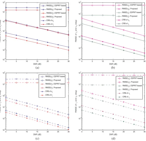
Figure 3. RMSE of the spatial and polarization angles of DOD and DOA. (a) RMSE ofθt andφt. (b)
essential for resolving the closely located targets.
Hereafter, in all the simulations, we considerL= 300 snapshots andK = 6 targets in whichKu= 1, Kp = 2, and D = 1 cluster with Kc = 3. The concerning reflectivities s1(l), sp(l) = [s2(l),s3(l)]T,
and sc(l) = s4(l)ρ1 are generated by the complex Gaussian with zero mean and unit variance. For
partially correlated targets, the correlation coefficient between s2(l) and s3(l) is set to 0.5. For
coherent targets, the correlation coefficient is set to one with ρ1 = [1, 0.2 + 0.84j, 0.4 + 0.7j]T. The
sequential angles are taken as θt = (10◦, 50◦, 45◦, 40◦, 25◦, 20◦), φt = (12◦, 24◦, 36◦, 30◦, 52◦, 48◦), γt =
(70◦, 50◦, 30◦, 20◦, 40◦, 60◦), ηt = (35◦, 11◦, 27◦, 51◦, 19◦, 43◦), θr = (8◦, 17◦, 22◦, 30◦, 42◦, 46◦), φr =
(14◦, 54◦, 40◦, 50◦, 23◦, 28◦), γr= (15◦, 35◦, 58◦, 75◦, 45◦, 25◦), andηr= (59◦, 21◦, 39◦, 49◦, 69◦, 79◦).
In the second simulation, shown in Fig. 3, root-mean-squared-error (RMSE) is measured and compared with the ESPRIT-based method [12] and the root CRB. The RMSE is defined by
RMSE =
1
McK
K k=1 Mc i=1
ψk−ψˆk,i
2
(16)
where ˆψk,i denotes the estimate of ψk ∈ (θtk,φtk,γtk,ηtk,θrk,φrk,γrk,ηrk) in the ith Monte-Carlo run,
andMcdenotes the total number of Monte-Carlo runs. The results in Fig. 3 signify that the performance
of the proposed approach follows the root CRB whereas performance of the ESPRIT-based method [12] is unsatisfactory, and constant floor occurs even at high SNR.
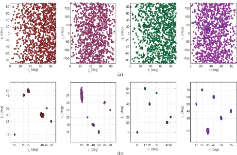
The next simulation illustrates the precision performance of the angle estimates using the scatter plot shown in Fig. 4. In Fig. 4(a), the estimated angles are spread randomly over the entire region. Thus, from Figs. 3 and 4(a), we signify that the ESPRIT-based method [12] fails to resolve the coherent
0 20 40 60 80 -80 -60 -40 -20 0 20 40 60 80
θt (deg)
φt
(deg)
0 20 40 60 80 -150 -100 -50 0 50 100 150
γt (deg)
ηt
(deg)
0 20 40 60 80 -80 -60 -40 -20 0 20 40 60 80
θr (deg)
φr
(deg)
0 20 40 60 80 -150 -100 -50 0 50 100 150
γr (deg)
ηr
(deg)
10 20 25 40 45 50 12 24 30 36 48 52
θt (deg)
φt
(deg)
20 30 40 50 60 70 11 19 27 35 43 51
γ (deg)
ηt
(deg)
8 17 22 30 42 46 14 23 28 40 50 54
θ (deg)
φr
(deg)
15 25 35 45 58 75 21 39 49 59 69 79
γr (deg)
ηr
(deg)
(a)
(b)
or mixed targets. However, in the proposed method shown in Fig. 4(b), the estimated angles of a particular target are close to the actual value.
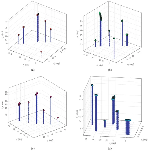
The final simulation, shown in Fig. 5, illustrates the conceivable three-dimensional stem plots for visualizing the pair-matching among all the eight parameters. For clearly identifying the location of the projected stems on the horizontal plane, grid-lines are highlighted only for the actual values of the concerning parameters. From the illuminated results in Fig. 5, one can notice that the spatial and polarization angles of DODs and DOAs of all targets are paired precisely.
50 45 40 46
15
42
t (deg)
25
25 30
r (deg)
20 35
22
r
(deg)
17 45
10 8
58 75
52 48 11
54 19
50 36
t (deg)
27
40 30
t
(deg)
35
r (deg)
24 43
28 24 51
12 14
12
75 24 30
58
t
(deg)
36
70 60
r (deg)
45 48
50 52
t (deg)
35 40
25 30
15 20
51 43 35
t (deg)
27 19 11 8
r (deg)
17
79 69
22
59
r
(deg)
49 39
30
21 42
46
(a) (b)
(c) (d)
Figure 5. Pair-matching among all the eight parameters. (a) Pairing of θt,θr and γr. (b) Pairing of
6. CONCLUSION
This paper constructs a more relevant scenario to the practical one that comprises a combination of uncorrelated, partially correlated, and the groups of coherent targets. In this scenario, we examine the importance of estimating multiple parameters like azimuth, elevation, and polarization angles for localization of the targets in bistatic MIMO radar. The proposed approach can locate any number of targets with pair-matching among all the parameters. Consequently, the proposed approach is practicable for the application where localization of the targets with multiple parameters estimations is essential.
REFERENCES
1. Li, J. and P. Stoica, “MIMO radar with colocated antennas,” IEEE Signal Processing Magazine, Vol. 24, No. 5, 106–114, 2007.
2. Zhang, X., X. Gao, G. Feng, and D. Xu, “Blind joint DOA and DOD estimation and identifiability results for MIMO radar with different transmit/receive array manifolds,”Progress In
Electromagnetics Research B, Vol. 18, 101–119, 2009.
3. Chen, H. W., D. Yang, H. Q. Wang, X. Li, and Z. W. Zhuang, “Direction finding for bistatic MIMO radar using EM maximum likelihood algorithm,”Progress In Electromagnetics Research, Vol. 141, 99–116, 2013.
4. Zheng, G. and B. Chen, “Unitary dual-resolution ESPRIT for joint DOD and DOA estimation in bistatic MIMO radar,” Multidimensional Systems and Signal Processing, Vol. 26, 159–178, 2015. 5. Jiang, H., J. K. Zhang, and K. M. Wong, “Joint DOD and DOA estimation for bistatic MIMO
radar in unknown correlated noise,” IEEE Transactions on Vehicular Technology, Vol. 64, No. 11, 5113–5125, 2015.
6. Wena, F., X. Xiong, J. Su, and Z. Zhang, “Angle estimation for bistatic MIMO radar in the presence of spatial colored noise,” Signal Processing, Vol. 134, 261–267, 2017.
7. Chen, H., X. Zhang, Y. Bai, and J. Ma, “Direction finding for bistatic MIMO radar with non-circular sources,”Progress In Electromagnetics Research M, Vol. 66, 173–182, 2018.
8. Zhang, W., W. Liu, J. Wang, and S. Wu, “Joint transmission and reception diversity smoothing for direction finding of coherent targets in MIMO radar,” IEEE Journal of Selected Topics in Signal
Processing, Vol. 8, No. 1, 115–124, 2014.
9. Srinivasarao, C. and P. Palanisamy, “DOD and DOA estimation using the spatial smoothing in MIMO radar with the EmV sensors,” Multidimensional Systems and Signal Processing, Vol. 29, No. 4, 1241–1253, 2018.
10. Chen, C. and X. Zhang, “A low-complexity joint 2D-DOD and 2D-DOA estimation algorithm for MIMO radar with arbitrary arrays,” International Journal of Electronics, Vol. 100, No. 10, 1455–1469, 2013.
11. Xia, T.-Q., “Joint diagonalization based 2D-DOD and 2D-DOA estimation for bistatic MIMO radar,”Signal Processing, Vol. 116, 7–12, 2015.
12. Srinivasarao, C. and P. Palanisamy, “2D-DOD and 2D-DOA estimation using the electromagnetic vector sensors,” Signal Processing, Vol. 147, 163–172, 2018.
13. Ye, Z., Y. Zhang, and C. Liu, “Direction-of-arrival estimation for uncorrelated and coherent signals with fewer sensors,”IET Microwaves, Antennas and Propagation, Vol. 3, No. 3, 473–482, 2009. 14. Liu, F., J. Wang, C. Sun, and R. Du, “Spatial differencing method for DOA estimation under
the coexistence of both uncorrelated and coherent signals,” IEEE Transactions on Antennas and
Propagation, Vol. 60, No. 4, 2052–2062, 2012.
15. Qin, S., Y. D. Zhang, and M. G. Amin, “DOA estimation of mixed coherent and uncorrelated targets exploiting coprime MIMO radar,”Digital Signal Processing, Vol. 61, 26–34, 2017.