Jamming Method Based on Optimal Power Difference for LMS-GPS
Receivers
Fulai Liu1, 2, Yadong Wang1, 2, *, Ling Yue1, 2, Xiaodong Kan1, 2, and Hui Song1, 2
Abstract—Jamming and anti-jamming techniques for global position systems (GPS) play important roles in electronic countermeasure. Least mean square (LMS)-based anti-jamming algorithm is widely used in GPS receivers, since it can avoid matrix inversion and has low complexity. For convenience, we call them LMS-GPS receivers. To improve the anti-jamming performance of the LMS-GPS receivers, it is very meaningful to study the jamming technique. Considering that existing jamming signals are easily suppressed by LMS-GPS receivers, a new jamming method named as optimal power difference jamming is proposed in this paper to improve the jamming effect further. Specifically, the analytical relationship between jamming-to-signal ratio (JSR) and the power difference of two interference signals is firstly given. Then, the conclusion that there is always an optimal power difference where the JSR can take the extreme value is drawn. Finally, the optimal power difference is derived as about 22 dB for single-tone interference and 29 dB for band-limited Gaussian noise interference. Simulation results show that the proposed method with optimal power difference is able to improve the JSR remarkably.
1. INTRODUCTION
Recently, the global position system (GPS) has become an indispensable part of daily life, which provides the position, velocity and timing information to enable many applications used in our daily life. Since the satellites are over 20,000 km away and are powered by solar cells, GPS signals have very low power to reach earth, thus, it is particularly vulnerable to intentional or unintentional interference [1]. Least mean square (LMS) algorithm is one of the most widely used anti-jamming algorithm because of its low complexity and better convergence performance. For convenience, we refer to a GPS receiver that uses the LMS algorithm for anti-jamming as an LMS-GPS receiver. In order to improve the anti-jamming performance of the LMS-GPS receiver, it is necessary to study the impact of interference.
Several anti-jamming algorithms have been proposed for GPS [2–9]. The affine combination of two LMS filters has a better performance compared to a single LMS filter, however, its computation cost is not attractive [2]. The performance of LMS algorithm without jamming is analyzed for different SNR environment in [3]. Variable step method is used to reach the fast convergence and a low steady state error in [4], which does not consider the interference problem. An approximate expression is presented in [5], which shows that the smaller LMS step size can decrease the mis-adjustment. Unfortunately, it may also cause a longer convergence time. A numerical analysis of the effect of carrier frequency on the signal-tone interference performance is given in [6]. A new variable step-size LMS algorithm is introduced in [7], which can provide fast convergence by adjusting the step size, however, the performance of this algorithm is highly depend on the criterion used to adjust the step size. The proportionate normalized LMS (PNLMS) adaptation algorithm is proposed in [8], which can improve the initial convergence by
Received 13 November 2018, Accepted 22 December 2018, Scheduled 8 January 2019
* Corresponding author: Yadong Wang (wangyadong [email protected]).
adjusting the step size of each filter coefficient. The anti-jamming LMS algorithms mentioned above ignore the influences of the interference signal power on the performance of these algorithms.
Meanwhile, most previous interference methods do not attach enough importance to the LMS-GPS receivers. They concentrate on producing code-tracking error, influencing acquisition performance, etc. For example, the influence of continuous wave (CW) interference on the acquisition performance of GPS receivers is analysed in [9]. Wideband interference has the best jamming effect on signal acquisition and tracking of the GPS receiver, which can cover the received signals and influence the performance of the GPS receiver [10]. In [11], the influence of CW jamming for the GPS receiver is analyzed, and the influence of Doppler frequency and integral duration is considered. The effect of band-limited Gaussian noise interference with different bandwidths, the influence of integration time and early-late spacing is assessed in [12].
In this paper, we propose a novel jamming method for LMS-GPS receivers. Firstly, the characteristics of the LMS anti-jamming algorithm are analyzed. And then, in view of the characteristics that the LMS algorithm will suppress higher power signal preferentially, the power difference between the two suppressed interference signals is adjusted to maximize output jamming-to-signal ratio (JSR) of the LMS-GPS receivers, which can ensure that the two interference signals have higher power in the received data of the LMS-GPS receivers. The proposed jamming method can obtain larger output JSR than one interference signal or two interference signals with the same power.
The rest of the paper is organized as follows. In Section 2, the system model of an LMS-GPS receiver is presented. The proposed jamming method is developed in detail and followed by the problem formulation in Section 3. Simulations have been performed to analyze the impact of different parameters on the power difference between the two suppressed interference signals in Section 4. Section 5 provides a concluding remark to summarize the paper.
2. SYSTEM MODEL
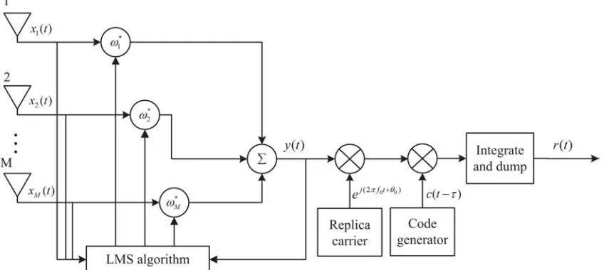
Consider a GPS receiver using the LMS anti-jamming algorithm as shown in Fig. 1, in which
x = [x1(t), x2(t), . . . , xM(t)]T denotes the received signal of array antenna; w = [w1, w2, . . . , wM]T represents the array weight vector;y(t) is the output signal of the received signal processed by the LMS algorithm, which is multiplied by the local carrier and the local C/A code to demodulate and dispread, and the data code of the GPS signal can be recovered by the integrate and dump.
The LMS algorithm is an adaptive beam forming algorithm, which has been widely used in the GPS receivers [13]. The optimal weights are obtained by iterative operations according to the minimum mean square error (MMSE). In general, the progress of the adaptive algorithm can be summarized as
follows: 1) Calculating the output of the array based on the received signal and the current weight vector. 2) Obtain the error between the output signal and the desired signal. 3) Adjusting the weight vector based on a certain rule. The above process is a continuous iterative process until meeting the requirements and reaching the steady state. The LMS algorithm can be described by the following equations
ε(n) = d(n)−wH(n)x(n) (1)
w(n+ 1) = w(n) + 2μx(n)ε(n) (2)
where d(n) is the desired signal; x(n) denotes the input signal vector at sampling timen; ε(n) stands for the deviation error;w(n) represents the filter coefficients vector; andμis equal to variable step [14].
μplays an important role in the performance of the proposed algorithm, which can influence the steady state error and convergence rate of LMS.
3. ALGORITHM FORMULATION
The received signal vector of array x(t) consists of one GPS signal, two interference signals and one noise signal, and it can be represented as
x(t) =a0(θ0)s0(t) +a1(θ1)j1(t) +a2(θ2)j2(t) +v(t) (3)
where a0(θ0), a1(θ1) and a2(θ2) denote the steering vectors of the GPS signal s0(t), two interference
signals j1(t) and j2(t), respectively. v(t) stands for the array noise vector. j1(t) and j2(t) have the
following forms
j1(t) =
P1s1(t) (4)
j2(t) =
P2s2(t) (5)
whereP1 andP2 denote the power ofj1(t) andj2(t), respectively; s1(t) ands2(t) are power normalized
interference signal; j1(t) is uncorrelated with j2(t). Introducing the notation ΔP =P1−P2, j2(t) can
be rewritten asj2(t) =
√
P1−ΔP s2(t).
Considering the relationship between the received signal and ΔP,x(t) can be given by
x(t) =a2
(P1−ΔP)s2(t) +c (6)
wherec=a0s0(t) +a1
√
P1s1(t) +v(t).
Above all, we give the following Theorem.
Theorem 1: For an LMS-GPS receiver, assume that the received signal includes a desired signal with a steering vector a0 and two interference signals with a power difference ΔP. If the receiver’s
weight vectorwsatisfies|wHa0|>0, then, there must be an interference signal power difference ΔPopt
such that the following equation holds
∂OJSR
∂ΔP
ΔP=ΔPopt
= 0 (7)
whereOJSR stands for the JSR of the received signal.
Proof: The desired signal’s output power P0out can be expressed as
P0out = lim T→∞
1
T T
0
|sdout(t)|2 dt
= lim T→∞
1
T T
0
wH(n)a0s0(t) 2
dt
= wH(n)a0 2
lim T→∞
1
T T
0
|s0(t)|2dt
= wH(n)a0 2
where sdout(t) =wH(n)a0s0(t), w(n) denotes the weight vector given by thenth iteration of the LMS
algorithm; a0 represents the desired signal steering vector; P0 stands for the input power of the GPS
signal.
Similarly, the output powers of two interference signals are
P1out =wH(n)a1 2
P1
P2out =wH(n)a2 2
P2. (9)
Combining Eqs. (8) and (9), the output JSR of signal is
OJSR= P1out
+P2out
P0out
= w
H(n)a12P1+wH(n)a22P2
|wH(n)a0|2P0
= w
H(n)a12P1+wH(n)a22(P1−ΔP)
|wH(n)a0|2P0 . (10) Assuming thatP0, P1,a0,a1,a2 are invariant, the relationship between signal output JSR and ΔP
can be expressed as
OJSR =
−aH2 w(n)wH(n)a2ΔP+
wH(n)a1 2
+wH(n)a2 2
P1
|wH(n)a0|2P0 . (11)
Considering the iterative solution process of the LMS algorithm,w(n)wH(n) can be written as
w(n)wH(n) = w(n−1)wH(n−1) + 2με(n−1)x(n−1)wH(n−1)
+2με∗(n−1)w(n−1)xH(n−1)
+4μ2ε(n−1)ε∗(n−1)x(n−1)xH(n−1)
= w(0)wH(0) + n
j=1
f(j) (12)
where
f(j) =A0(j)(P1 −ΔP) +B0(j)
P1−ΔP +C0(j)
A0(j) =
j
i=1
4μ2ε(j−1)ε∗(j−i)a2aH2 s2(j−1)s∗2(j−i)
+ j
i=2
4μ2ε∗(j−1)ε(j−i)a2aH2 s2(j−i)s∗2(j−1)
B0(j) = 2με(j−1)a2s2(j−1)wH(0) + 2με∗(j−1)w(0)aH2 s∗2(j−1)
+ j
i=1
4μ2ε(j−1)ε∗(j−i)a2cHs2(j−1) +ca2Hs∗2(j−i)
+ j
i=2
4μ2ε∗(j−1)ε(j−i)a2cHs2(j−i) +caH2 s∗2(j−1)
C0(j) = 2με(j−1)cwH(0) + 2με∗(j−1)w(0)cH
+ j
i=1
4μ2ε(j−1)ε∗(j−i)ccH+ j
i=2
4μ2ε∗(j−1)ε(j−i)ccH
Substituting Eq. (12) into Eq. (11), we have
OJSR=
A1(n)(P1−ΔP)2+B1(n)(P1−ΔP) 3
2+C1(n)(P1−ΔP)+D1(n)(P1−ΔP) 1
2 +E1(n)
F1(n)(P1−ΔP) +H1(n)(P1−ΔP) 1
2 +M1(n)
(14)
where
A1(n) =aH2
n
m=1
A0(m)a2
B1(n) =aH2
n
m=1
B0(m)a2
C1(n) =aH2 w(0)wH(0)a2+aH1
n
m=1
A0(m)a1P1+aH2
n
m=1
C0(m)a2
D1(n) =aH1
n
m=1
B0(m)a1P1
E1(n) =aH1 w(0)wH(0)a1P1+aH1
n
m=1
C0(m)a1P1
F1(n) =aH0
n
m=1
A0(m)a0P0
H1(n) =aH0
n
m=1
B0(m)a0P0
M1(n) =aH0 w(0)wH(0)a0P0aH0
n
m=1
C0(m)a0P0.
(15)
For convenience, we define P1−ΔP =x2, and OJSR can be rewritten as
OJSR =
A1(n)x4+B1(n)x3+C1(n)x2+D1(n)x+E1(n) F1(n)x2+H1(n)x+M1(n) .
(16)
The derivative ofOJSR can be given by
∂OJSR
∂x =
ax5+bx4+cx3+dx2+ex+f
(F1(n)x2+H1(n)x+M1(n))2
(17)
where
a= 2A1(n)F1(n), b=B1(n)F1(n) + 3A1(n)H1(n), c= 2B1(n)H1(n), d= 2B1(n)H1(n) + 4A1(n)M1(n), e= 2C1(n)M1(n)−2E1(n)F1(n), f =D1(n)M1(n)−E1(n)H1(n).
(18)
Since the denominator in Eq. (17) is always greater than zero, and the highest power of the numerator polynomial is 5, i.e., it must have 5 roots, it is easy to know that the numerator polynomial has at least one real root because the complex roots appear in pairs. Therefore, there is at least one real number in Eq. (17) such that the first-order derivative of OJSR is zero. Thus we have
∂OJSR
∂x
x=x0
= 0 (19)
Owing to ΔP =P1−x2, there must be a ΔP satisfying the following expression
∂OJSR
∂ΔP
ΔP=ΔPopt
This concludes the proof.
Theorem 3.1 shows that in Eq. (16), there must be a ΔPopt satisfying Eq. (20), and the ΔPopt is
called Stationary Point. Therefore, we can reasonably speculate that the stationary point may be a maximum or minimum point.
Next, we will use the simulation to further study the relationship between output JSR and ΔP. Assume that the uniform linear array (ULA) consists of five sensors (M = 5) spaced by half-wavelength, and the number of snapshots isL= 400. Assuming that there are one GPS signal and two single-tone interference signals, their center frequencies and directions are f0 = 1.575 GHz, θ0 = 20◦, f1 = 1.574 GHz, θ1 = −40◦, f2 = 1.5755 GHz, θ2 = 60◦, respectively. In this simulation, the
signal-to-noise-ratio (SNR) is set to −20 dB and 60 dB for the GPS signal and the first interference signal, respectively, and the SNR of the second interference signal changes from 0 dB to 60 dB.
Figure 2 plots the the output JSR versus ΔP. It can be seen that there is a maximum when ΔP
changes from 0 dB to 60 dB, and this result matches Theorem 1. On the other hand, Fig. 2 shows that the optimal power difference of single-tone interference is about 22 dB.
0 10 20 30 40 50 60
25 30 35 40 45 50 55
ΔP/dB
Output JSR/dB
Figure 2. The output JSR versus ΔP.
Through the above theoretical analysis and simulation result of Fig. 3, the following conclusion can be drawn: we can maximize the signal output JSR by finding an optimal power difference ΔPopt. That
is, when two interference signals with different powers are used to interfere with the LMS-GPS receiver, there must be an optimal interference power difference so that the received signal has the largest output JSR after being processed by the LMS algorithm. From the conclusion, we give an interference method named as jamming method based on optimal power difference (OPD-LMS), in which two interference signals are utilized, and the power difference between the two interference signals is set to ΔPopt.
4. SIMULATION RESULTS
In this section, we construct several simulations to demonstrate the effectiveness of the proposed algorithm. Consider a ULA with M antenna elements, in which M = 5, d/λ = 1/2, d is element spacing, and λis wave length. Assuming that there are three signals impinging on the antenna array, the frequency of the desired signal is f1 = 1.575 GHz, and the center frequencies of the two interferer
signals are f2 = 1.574 GHz and f3 = 1.5755 GHz, respectively. Their DOAs are θ1 = 20◦, θ2 = −40◦,
and θ3= 60◦, respectively.
0 10 20 30 40 50 60 70 80 10
20 30 40 50 60 70 80
ΔP/dB
Output JSR/dB
80dB 60dB 40dB 30dB
Figure 3. The output JSR versus single-tone interference’s input power.
interference. We set the first interference power as P1 = 30 dB, 40 dB, 60 dB and 80 dB, respectively,
and the ΔP changes from 0 dB toP1. It is easy to know that for different values of P1, there is always
a maximum in output JSR. Therefore, we can conclude that though P1 affects the output JSR of the
signal processed by the LMS algorithm, the optimal interference power difference ΔPopt is almost not
changed, that is to say,P1 has no effect on ΔPopt.
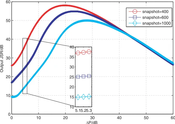
Figure 4 plots the output JSR versus snapshots. In brief, the snapshots impact the output JSR of signal significantly. On the one hand, when the snapshots are 400, 600, 1000, respectively, as the ΔP increases, there is a maximum point in their output JSR, but their value is different. On the other hand, the maximum output JSR depends on the number of snapshots, that is, as the snapshots increase, the maximum JSR decreases. The reason may be that the anti-interference performance of the LMS algorithm significantly increases as the snapshots increase, which causes the output JSR to decrease. Therefore, we can conclude that, as the snapshots increase, the output JSR decreases, and ΔPopt increases, but it can also get an ideal output JSR when ΔP = 22 dB.
Figure 5 gives the output JSR versus band-limited Gaussian noise interference’s input power.
0 10 20 30 40 50 60
0 10 20 30 40 50 60
ΔP/dB
Output JSR/dB
5.15.25.3 10 15 20 25 30 35 40
snapshot=400 snapshot=600 snapshot=1000
0 10 20 30 40 50 60 70 80 20
30 40 50 60 70 80
ΔP/dB
Output JSR/dB
80dB 60dB 50dB 45dB 40dB
Figure 5. The output JSR versus band-limited Gaussian noise interference’s input power.
30 35 40 45 50 55 60 65 70 75 80 0
10 20 30 40 50 60 70 80
input INR/dB
Output JSR/dB
OPD-LMS method
two single tone interferences with same INR one single tone interference
Figure 6. The output JSR versus the input INR in different interference methods.
Similar to Fig. 3, we also considerP1 = 40 dB, 45 dB, 50 dB, 60 dB and 80 dB, respectively, and the ΔP
changes from 0 dB to P1. When the interference signal is band-limited Gaussian noise interference, we
can see that they all have the maximum, but unlike Fig. 3, the optimal power difference is about 29 dB. Therefore, we have the following conclusion: the optimal power difference of band-limited Gaussian noise interference is about 29 dB.
5. CONCLUSION
In this paper, a new interference method for the LMS-GPS receiver is presented. The proposed jamming method includes two interference signals, and they have a optimal power difference ΔPopt. Through
theoretical and simulation analysis, the optimal power difference ΔPopt is derived as about 22 dB for
single-tone interference and 29 dB for band-limited Gaussian noise interference. Compared to one interference signal and two identical power interference signals, the presented method gets a higher JSR and has better jamming performance.
ACKNOWLEDGMENT
This work was supported by the Natural Science Foundation of Hebei Province (No. F2016501139), by the Fundamental Research Funds for the Central Universities under Grant (Grant No. N172302002, Grant No. N162304002), and by the National Natural Science Foundation of China (Grant No. 61501102).
REFERENCES
1. Pinker, A. and C. Smith, “Vulnerability of the GPS Signal to Jamming,” GPS Solutions, Vol. 3, No. 2, 19–27, 1999.
2. Kamatham, Y., B. Kinnara, and M. K. Kartan, “Mitigation of GPS multipath using affine combination of two LMS adaptive filters,” IEEE International Conference on Signal Processing, Informatics, Communication and Energy Systems, Vol. 35, 1–4, 2015.
3. Ahmad, Z., M. Tahir, and I. Ali, “Analysis of beamforming algorithms for antijams,”2013 XVIIIth International Seminar/Workshop on Direct and Inverse Problems of Electromagnetic and Acoustic Wave Theory (DIPED), 89–96, 2013.
4. Chan, S. C. and Y. Zhou, “Improved generalized-proportionate stepsize LMS algorithms and performance analysis,”IEEE International Symposium on Circuits and Systems, 2325–2328, 2006. 5. Gardner, W., “Nonstationary learning characteristics of the LMS algorithm,” IEEE Transactions
on Circuits and Systems, Vol. 34, No. 10, 1199–1207, 2003.
6. Luo, H., “Accurate analysis of processing gain in direct sequence spread spectrum communication systems under single-tone and narrowband interference,”Telecommunication Engineering, 2014. 7. Pazaitis, D. I. and A. G. Constantinides, “A novel kurtosis driven variable step-size adaptive
algorithm,”IEEE Transactions on Signal Processing, Vol. 47, No. 3, 864–872, 1999.
8. Duttweiler, D. L., “Proportionate normalized least-mean-squares adaptation in echo cancelers,”
IEEE Transactions on Speech and Audio Processing, Vol. 8, No. 5, 508–518, 2002.
9. Ye, F., H. Tian, and F. Che, “CW interference effects on the performance of GPS receivers,” 2017 Progress In Electromagnetics Research Symposium — Fall (PIERS — FALL), 66–72, 2017. 10. Mao, Y. and C. Guo, “Analysis of interference effect on signal acquisition and tracking of GPS
receiver,” IEEE International Conference on Communication Problem-Solving, 592–595, 2014. 11. Balaei, A. T., A. G. Dempster, and L. L. Presti, “Characterization of the Effects of CW and Pulse
CW Interference on the GPS Signal Quality,” IEEE Transactions on Aerospace and Electronic Systems, Vol. 45, No. 4, 1418–1431, 2009.
12. Betz, J. W. and K. R. Kolodziejski, “Generalized theory of code tracking with an early-late discriminator Part II: Noncoherent processing and numerical results,” IEEE Transactions on Aerospace and Electronic Systems, Vol. 45, No. 4, 1557–1564, 2009.
13. Liu, F., R. Du, and X. Bai, “A virtual space-time adaptive beamforming method for space-time antijamming,”Progress In Electromagnetics Research M, Vol. 58, 183–191, 2017.